Geometric Accuracy of Sentinel-1A and 1B Derived from SAR Raw Data with GPS Surveyed Corner Reflector Positions


Microwaves and Radar Institute, German Aerospace Center (DLR), 82234 Oberpfaffenhofen, Germany
*
Author to whom correspondence should be addressed.
Remote Sens. 2018, 10(4), 523; https://doi.org/10.3390/rs10040523
Submission received: 22 December 2017
/
Revised: 21 March 2018
/
Accepted: 23 March 2018
/
Published: 27 March 2018
Abstract
:The geometric accuracy of synthetic aperture radar (SAR) data is usually derived from level-1 products using accurately surveyed corner reflector positions. This paper introduces a novel approach that derives the range delay and azimuth shift from acquired SAR raw data (level-0 products). Therefore, the propagation path is completely retrieved from SAR pulse transmission up to the reception of the point target’s backscatter. The procedure includes simple pulse compression in range and azimuth instead of full SAR data processing. By applying this method, the geometric accuracy of ESA’s Sentinel-1 SAR satellites (Sentinel-1A and Sentinel-1B) is derived for each satellite overpass by using corner reflectors with precisely surveyed GPS positions. The results show that the azimuth bias of about 2 m found in level-1 products for Stripmap acquisitions is reduced to about 15 cm. This indicates an artificial bias arising from operational Sentinel-1 SAR data processing. The remaining range bias of about 1.0 m, observed in L0-products, is interpreted as the offset between the SAR antenna phase center and the spacecraft’s center of gravity. The relative pixel localization accuracy derived with the proposed method is about 12 cm for the evaluated acquisitions. Compared to the full processed level-1 SAR data products, this accuracy is similar in the range direction, but, for the azimuth direction, it is improved by about 50% with the proposed method.

1. Introduction
Synthetic aperture radar (SAR) images are commonly used for Earth observation. In contrast to optical systems, SAR instruments can be operated more independently from temporal (day or night) and meteorological conditions. The spatial resolution of SAR images has also been improved for space-borne missions down to values in the order of meters and sub-meters in both the range and azimuth directions [1,2]. To ensure a geometric accuracy in the same order of magnitude, the geocoding step as part of the SAR data processor becomes a more challenging task, which includes a precise characterization of the measurement system and ancillary information like orbit accuracy, digital elevation models (DEMs) used as input, etc. In general, additional parameters or look-up tables are delivered in combination with SAR data products to allow the association of any pixel in the given SAR image with a geographical position on the Earth’s surface. However, for precise geolocation of SAR data products, the range-Doppler equations have to be solved using the annotated range and azimuth time as well as precise orbit data.
The Sentinel-1 mission in the frame of ESA’s COPERNICUS program aims to ensure long-term Earth observation under stable conditions. Both satellites Sentinel-1A (S-1A) and Sentinel-1B (S-1B) are operated in a near polar sun-synchronized orbit, each with a repeat cycle of 12 days, in such a way that the two satellite constellation offers a 6-day repeat cycle over a given observation area. Both SAR instruments operate at C-band (with a center frequency of 5.405 GHz) and carry a right-looking active phased array antenna. Dual polarization operation (HH+HV, VV+VH) is realized by one transmit chain (switchable to H or V) and two parallel receive chains, one for H and one for V polarization. Sentinel-1 provides different operation modes: Stripmap, Interferometric Wide swath (IW), Extra-wide swath (EW) and Wave mode. The six available Stripmap beams have a swath width of 80 km each with a spatial image resolution of 5 m by 5 m. For IW and EW acquisitions, the instrument is operated in the Terrain Observation with Progressive Scan (TOPS) mode [3] by steering the antenna electronically from backwards to forwards for each burst. Compared to Stripmap, this technique enables the observation of a larger swath width of 250 km for IW mode and of 400 km for EW mode; the spatial resolution is accordingly reduced to 5 m by 20 m and 20 m by 40 m, respectively [4,5].
The geolocation accuracy of space-borne SAR instruments, also known as pixel localization accuracy, has to be determined using the range-Doppler equations [6] and verified by analyzing SAR images [7,8,9]. To achieve and verify a high spatial accuracy of below one meter, the related geometric conditions have to be known very accurately, e.g., the spacecraft orbit, the SAR antenna geometry related to the spacecraft’s center of gravity and reference points precisely surveyed on the ground. Moreover, SAR data processing has to consider all relevant timing issues that are relevant for focusing the SAR image in range and azimuth [10], which could likewise arise from the instrument internal delay or from the used interpolation, approximation and signal filtering technique. Furthermore, the wave propagation is affected by the atmosphere; considerable delays are induced by the troposphere and ionosphere [11] and need to be considered accordingly. In particular for TerraSAR-X, a geospatial accuracy of SAR images in the centimeter domain, below a tenth of the resolution cell, was reported [7,8,12,13].
The pixel localization accuracy of both S-1A and S-1B was analyzed during their respective commissioning and routine operation phases within several studies [14,15,16,17] by evaluating the SAR images (L1 products) processed with Sentinel-1’s operational SAR Instrument Processing Facility (IPF). The relative pixel localization accuracy, which is the standard deviation for the absolute location error, has been determined to be below 0.5 m in range and azimuth, in particular for Stripmap mode. However, for all four studies, an offset in azimuth of about 2 m was found. In all cases, the azimuth time derived from SAR data precedes the predicted overpass time given by precise orbit data. The reason for this azimuth bias could arise from inaccurate SAR data processing or from non-considered additional geometric offsets like a significant distance between the spacecraft’s center of gravity and the SAR antenna phase center.
In order to address this issue, this paper proposes a new and easily applied method to verify the geometric accuracy based on SAR raw data (L0). The method analyzes the timing information from L0 raw data and compares it to the target responses of precisely surveyed point targets before (an explicit) SAR data processing is applied. The method includes simplified range and azimuth compression procedures and focuses mainly on selected data, which contain the target response. The purpose of this method is twofold: on the one hand, the potential geometric accuracy of SAR products is evaluated and, on the other hand, the geometric results after SAR data processing can be cross-checked and analyzed. This helps to detect potential error sources that may have been introduced to L1 products during SAR data processing.
2. Method
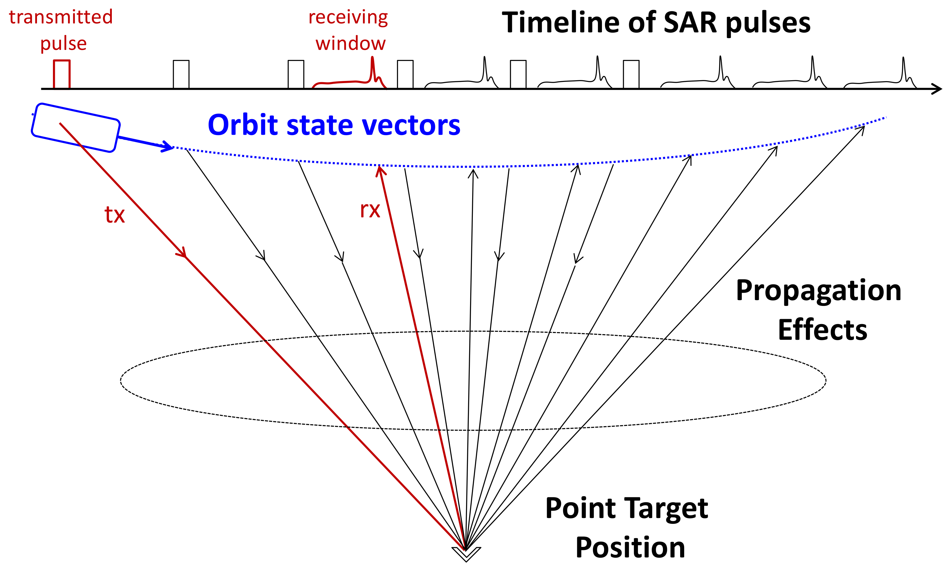
In order to verify the geometric properties of the SAR products, the signal propagation path has to be completely retrieved: from transmitting the SAR pulses up to receiving the backscatter power from the point target. The main parameters to be considered are depicted in Figure 1: the geometry between spacecraft and point target is determined by the orbit state vectors and the point target position on Earth. The information about transmitted and received pulses is saved by the SAR instrument as a timeline in the SAR raw data headers. Along the propagation path, the pulses are affected by several effects (mainly due to the troposphere and the ionosphere), which cause additional delays and need to be considered.
The proposed method evaluates the SAR pulse propagation time by using the speed of light and the interpolated positions of the SAR antenna, which are related to the position of the spacecraft. The exact position of the point target’s phase center is precisely surveyed by differential GPS.
2.1. Impulse Response Extraction of a Range Line
The transmission pulse of Sentinel-1 is a chirp signal defined by a pulse length, a start frequency and a frequency ramp rate. The time range between subsequent transmission pulses is indicated by the pulse repetition interval (PRI). The received signal is acquired within a certain sampling (or receiving) window between two successive transmission pulses. This sequence of samples is stored for each received signal as a range line. The reciprocal of the range sampling rate defines the time interval between consecutive samples of a range line; the related time axis is called range or fast time.
The round trip time () defines the pulse propagation time as detected by the SAR instrument. It can be derived for each sample of a range line using Equation (1). The is the number of PRIs between the pulse transmission and the corresponding reception of its echo. The start time of the receiving window within the PRI is considered by ; represents the fast time within the receiving window of the related pulse echo:
In order to extract the impulse response from L0 data, the received signal is correlated with an ideal chirp (match filter) in the time domain. The output gives the range compressed signal with complex values for the full range line. As the study focuses rather on propagation times and related phases than on absolute backscattering power, no gain normalization steps are required for this approach. Note that, in general, the matched filter procedures for SAR data processing are transferred to the frequency domain to optimize the performance of the calculations [18], but with the same expected results. This frequency domain approach is also used for the operational Sentinel-1 SAR processor.
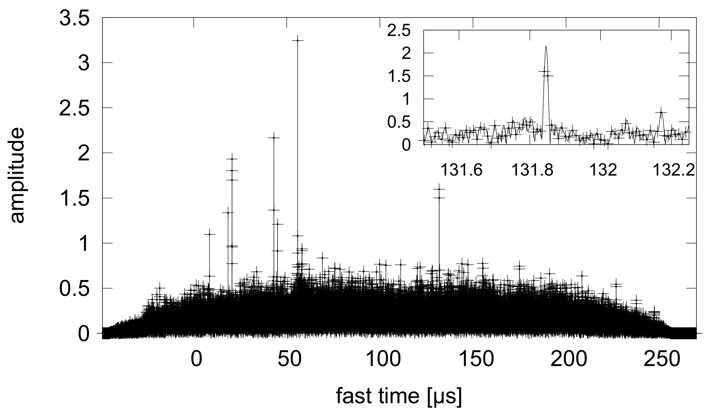
A high radar backscatter due to a transponder or corner reflector is easily detectable within the range compressed signal. Within the complex data stream, the target responses show a higher amplitude compared to the background noise as depicted for the corner reflector response at 131.84 s in Figure 2. Furthermore, the signal propagation time of the detected pulse can be (roughly) estimated by using the annotated timestamp of the first sample, the range sampling frequency and the sample number containing the target response. This information is used to identify the related target response as the (local) maximum amplitude within the receiving window. To achieve a higher resolution for the receiving time , the complex data is interpolated within a certain range around the peak.
The peak amplitude of the interpolated data is determined for each analyzed range line; the corresponding phase and the range time are stored for the analysis of the offsets in range and azimuth.
2.2. Range Offset
In order to verify the round trip time measured by the SAR instrument (), the predicted propagation time () is derived from the geometry. For this purpose, the spacecraft position () is estimated for both timestamps, first by the pulse transmission () and second by its reception () as depicted in Equation (2). With the known target position on ground (), the signal propagation path length is estimated as the sum of the transmission and the reception path and converted into a propagation time by dividing through the speed of light:
The range delay offset results from the difference between the signal propagation time () measured by the SAR instrument and the predicted one (). These offsets are analyzed not only for a single range line, but for a set of subsequent pulses with a sufficient signal-to-noise ratio for the target response.
Additional effects that extend the signal propagation have to be considered, mainly the internal delay of the SAR instrument itself and the atmospheric delay caused by the troposphere and ionosphere. The atmospheric corrections can be derived from the zenith path delay (ZPD) and the total electron content (TEC), both measured by nearby reference stations (see Section 4.2). The remaining range delay offset is converted into a geometric range offset by multiplying by half the speed of light, which considers the two-way pulse propagation.
2.3. Azimuth Offset
In order to derive an offset in azimuth direction, the phase history of a specific target is traced during an overpass. Therefore, the detected phase of complex SAR data containing the target response is compared with the predicted phase derived from the geometry using orbit data. This is done by converting the propagation time () between satellite and reference target into a phase value using the radar frequency () as given in Equation (3):
The backscatter from a point target is shifted in frequency by an amount proportional to the relative velocity between satellite and target . This Doppler frequency is described by the SAR Doppler Equation (4) and related to the phase by = −d / dt:
The Doppler frequency changes its sign when the spacecraft passes the target. At , the minimum distance between spacecraft and target is reached. We define this time as reference time . For , the satellite moves in the direction toward the target; for , the satellite moves away from it. It should be noted that the spacecraft attitude and the antenna pointing have no impact on the Doppler frequency in Equation (4) and the geometric phase in Equation (3), which are related to the spacecraft’s center of gravity. An antenna mispointing impacts the transmitted and received gain of the antenna w.r.t. the target direction but not the measured phases of pulses containing the target response. The relative motion between the antenna phase center and the spacecraft’s center of gravity is very small for Sentinel-1 and negligible for our study. Thus, the proposed method for deriving the azimuth offset focuses on phases not on amplitudes and verifies the azimuth time of the acquired target phase history using the related geometry including orbit state vectors and target position.
Figure 3 (top) depicts the phase history of a point target for a single overpass. The observed SAR data phase shown in blue is wrapped with values between −180 and 180; the predicted phase (black line) is overlaid presuming the same phase offset at . The maximum of the predicted phase (related to shortest propagation time ) corresponds to the minimum distance between satellite and target, which is expected at . By subtracting the predicted geometric phase from the measured SAR data phase, a low difference less than 5 remains in this case as depicted in Figure 3 (bottom). Note that, if the phase difference is computed using complex math an explicit phase, unwrapping is not necessary. The low variation and the absence of a ramp within the phase difference indicate that the azimuth timing measured by the SAR instrument matches well with that derived by the geometry; consequently, no significant azimuth offset is expected after azimuth compression.
The azimuth compression is performed with a matched filter focusing on the phase. For this task, the measured phase history is correlated with the one predicted from geometry. For our analysis, it is sufficient to use the target response derived from the maximum amplitude of each range line (as seen in Figure 3) instead of composing a two-dimensional, full focused SAR image. The correlation result contains the azimuth compressed data as a function of azimuth shift, i.e., the difference between measured and predicted phase history. The azimuth shift can be directly converted to an azimuth offset (in meters) by multiplying with the satellite velocity on ground (~6836 m/s for Sentinel-1).
The amplitude of azimuth compressed data as a function of the azimuth offset is depicted in Figure 4. A maximum value on the x-axis origin indicates that the measured phase (from L0 data) matches with the predicted geometry from orbit data as seen for precise orbit (solid line). An azimuth shift occurs if the measured and predicted phases are shifted in time relative to each other. This could be caused by an inaccurate geometry (orbit or target) or imprecise timing information. Using a predicted orbit, which was available before the acquisition has been acquired, an azimuth offset of 4.8 m remains (dashed line in Figure 4). This offset corresponds to an orbit shift in time of about 700 s. In contrast to the well balanced case depicted in Figure 3 (bottom), the predicted orbit introduces a remaining linear phase ramp in this case. The matched filter output from azimuth is complex interpolated to improve the resolution and thus to increase the accuracy of the azimuth offset result derived for each dataset.
3. Measurement Campaign
3.1. Observation Period
Two dedicated calibration campaigns were performed with Stripmap mode acquisitions using corner reflectors of the calibration site from the German Aerospace Center (DLR). Each campaign was covered by six repeat cycles of Sentinel-1. The S-1A campaign took place between August and October 2015, the S-1B campaign between December 2016 and February 2017 (see Table 1).
In case of S-1A, only the Stripmap beams S1, S3, and S6 were acquired for both orbit directions, the ascending (ASC) and descending (DES) orbits. For S-1B, all six Stripmap beams were used (S1 to S6), but each one of them was used either with the ASC or DES orbit direction. The selection of the Stripmap beams ensures a maximum number of S-1 overpasses across the DLR calibration site with six per repeat cycle, i.e., in summary, 72 acquisitions (for both satellites) were evaluated for this study.
3.2. Estimation of Point Target’s Phase Center
The DLR calibration site, located in Southern Germany, has already been used for geometric, radiometric and polarimetric calibration of a number of space-borne SAR missions like TerraSAR-X, TanDEM-X, S-1A and S-1B [19]. For the current study, the three remotely controlled and configurable corner reflectors were used as reference targets. For a given overpass, each of these targets can be automatically aligned using an individual schedule configured from a remote station. For a planned acquisition, the exact overpass time as well as alignment angles in azimuth and elevation are determined using spacecraft predicted orbit data.
The exact phase center position (latitude, longitude, height) for each corner reflector is calculated from a model considering the corner reflector’s geometry and the individual adjusted configuration for each acquisition. The geometric accuracy of the model has been validated for all three corner reflectors by evaluating a number of individual measured GPS target positions at each site. The geometric deviations are converted into a local coordinate system (x, y, z); the accuracy results for each target are summarized in Table 2.
Low deviations in the order of a centimeter have been determined between the measured and predicted phase center positions for all three dimensions (dx, dy and dz column in Table 2). This confirms that no significant bias remains in a specific direction. The absolute position error () has been estimated by calculating the mean square root for each target. The remaining absolute position error is below 3 cm for all targets. The orbit accuracy for the precise orbit determination has been verified to fulfill the requirement of 5 cm in 3D [20]. Note that the absolute target position is finally converted to the same reference frame, which is also used for Sentinel-1 by the orbit data (ITRF 2008).
4. Impacts on the Range Delay
4.1. Internal Delay of the SAR instrument
The internal delay of the SAR instrument is derived by using internal calibration pulses. A set of 300 calibration pulses is acquired before and after each Sentinel-1 Stripmap acquisition. Evaluation of these calibration pulses serves to derive the instrument internal delay. This delay is calculated for each overpass and considered as an individual input parameter for range delay estimation.
The instrument internal delay is found to be very stable for each Sentinel-1 instrument over both observation periods. For S-1A, a mean instrument internal delay of 441.6 ns with a small variation of 0.5 ns is derived for the analysis period (August–October 2015). Similar results are obtained for S-1B (acquired during its analysis period December 2016–February 2017) with a mean instrument internal delay of 433.7 ns and a variation of 0.3 ns. These values are consistent with the instrument internal delay determined by the operational processor (IPF), which are annotated within the L1 products.
4.2. Tropospheric Delay
The Regional Reference Frame Sub-Commission for Europe (EUREF) operates a permanent network of reference stations with precisely known coordinates using global navigation satellite systems (GNSS). For the current study, the measured zenith path delay () is used which is provided by EUREF [21]. The data tracked by each EUREF station can be downloaded via ftp from the EUREF website. The measured delay is converted into a height corrected zenith path delay () by using the station altitude () and Equation (5) with a reference height () of 8000 m:
Figure 5 shows the total delay from height corrected data for two EUREF stations close (<120 km) to the DLR calibration field (OBE4: Oberpfaffenhofen, Germany, PFA2: Bregenz, Austria). The left sub-figure focuses on S-1A acquisitions and covers an observation period of one month during the late summer 2015 where a ZPD of about 2.45 m is found on average. The right sub-figure depicts the period of S-1B acquisitions early 2017 with a mean ZPD of about 2.4 m. Although seasonal and daily variations of ZPD values in the order of a few 10 cm exists, the spatial variation is much slower. Both EUREF stations, with a distance of 150 km in between, show a similar trend with low ZPD differences below 1 cm. For the current study, a specific ZPD value is derived for each satellite overpass by using the best matching ZPD value in time for the GNSS station OBE4 (nearest neighbor).
The additional range offset due to tropospheric effects () is then calculated with Equation (6) using the altitude at the corner reflector location () and the incidence angle () of the SAR satellite for this position. As the temporal resolution of the delivered ZPD values is one hour and the distance from the reference station to the related corner reflector is between 40 and 110 km, an uncertainty in the order 1 cm is expected for the tropospheric delay contribution. The tropospheric delay, which is to be considered within the evaluation, can be calculated by multiplying the related path length with half the speed of light:
4.3. Ionospheric Delay
An additional delay suffers the signal along the propagation path due to the electron content within the ionosphere. This ionospheric delay is estimated by multiplying half the speed of light with the frequency dependent range offset from Equation (7) taking into account the carrier frequency f of the radar. In order to determine the electron content in slant range, the vertical total electron content (VTEC) has to be divided by the cosine of the incidence angle ():
Several models exist for retrieving VTEC values for a given time and geographic position (latitude, longitude) using the measurement of a ground based station network. For the current study, an empirical electron density model called International Reference Ionosphere (IRI) 2012 has been used [22]. The model output to a given time and location is available via website, e.g., at https://omniweb.sci.gsfc.nasa.gov/vitmo/iri2012_vitmo.html. Based on these VTEC values, the ionospheric delay has been derived for each overpass according to Equation (7).
It is found that the impact of the ionosphere is slightly different for the two observation periods. For S-1A, the delays vary from 0.6 ns to 1.4 ns with an average value of 1.0 ns and a standard deviation of 0.3 ns. For S-1B, the ionospheric activity is lower; delays between 0.14 ns and 0.56 ns have been detected with 0.3 ns in average and a standard deviation of 0.1 ns. The contribution of the ionosphere to the range offset is estimated to be 1 cm for S-1A and 0.4 cm for S-1B with a small uncertainty of 0.3 cm and 0.15 cm for S-1A and S-1B, respectively.
Note that, for low orbit satellites, the SAR pulse does not travel through the full ionosphere. This fact leads to an overestimation of the ionospheric delay with Equation (7). However, this additional correction is neglected in our study due to the small impact of the ionospheric delay for the C-band.
5. Results
5.1. Range Offset from Corner Reflectors
The determined range offset from L0 data is depicted in Figure 6 (blue) for both satellites (S-1A: left and S-1B: right). In addition, the range offset from the L1 products are also displayed (black), which were already presented in previous studies [14,15,16,17]. An averaged range offset of −0.99 m remains for the S-1A L0 products and of −1.05 m for the S-1B ones. These results match the offset between the spacecraft’s center of gravity and SAR antenna phase center, which is the order of 1 m and not considered for the L0 evaluation. After compensating for these offsets, the remaining standard deviation is a measure for the pixel localization in range, which is 12 cm for S-1A and 7 cm for S-1B.
The range offsets derived from L1 products are smaller than the ones derived from L0 products. There is one exception though: the S-1B Stripmap beam S1 shows a larger offset with 1.6 m and indicates an inaccurate set of SAR processing parameters for this beam. The difference between L0 and L1 products is on average 1.3 m for S-1A and of 1.2 m for S-1B (excluding the S1 beam results). Furthermore, the variation of the range offset for L1 products is nearly identical to the one derived from L0 products. Although no explicit indication is found in the L1 product annotation files, the small values of the L1 derived range offsets evidence that the distance between spacecraft’s center of gravity and SAR antenna phase center is already considered during SAR data processing.
5.2. Azimuth Offset from Corner Reflectors
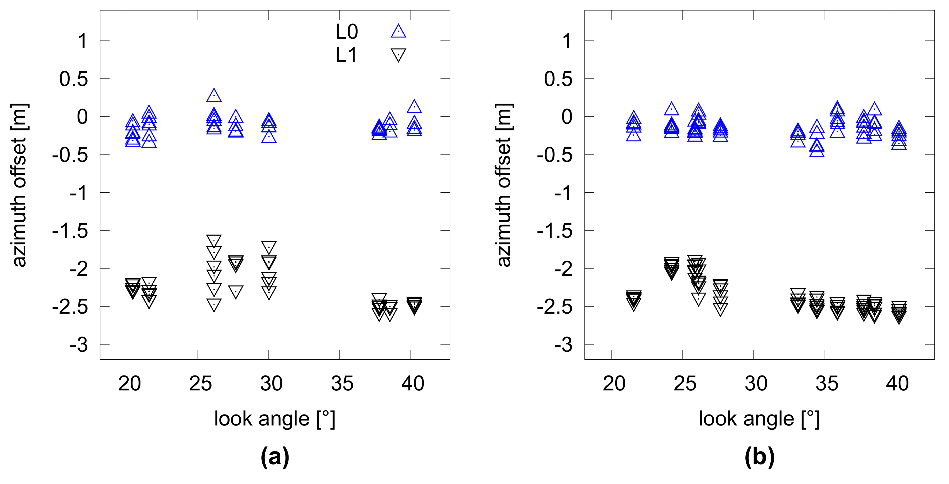
The derived azimuth offset is depicted in Figure 7 using L0 data (blue points) for both satellites (S-1A: left and S-1B: right). Similar to the range results, the azimuth offsets derived from L1 products are also shown (black points). For the L0 products, a very small azimuth offset remains, with −11 cm on average for S-1A and −14 cm for S-1B. After compensating for these offsets, the standard deviation is a measure of the pixel localization accuracy in azimuth, which is derived from L0 products to 12 cm for both satellites.
In contrast to these results, the analysis performed using L1 products shows a remaining bias of m for both S-1A and S-1B. Note that these results are consistent with other previous studies [14,15,16,17], in which similar values were obtained. This remaining azimuth bias for L1 products corresponds to an azimuth shift of about half the pulse repetition interval. As the proposed method does not perform SAR azimuth processing, it is assumed that such an azimuth bias of L1 products is artificial and probably arises due to an incorrect azimuth shift during operational SAR data processing.
The statistics of the derived pixel localization accuracy with mean value and standard deviation are summarized in Table 3 separately for range and azimuth offset. Similar to Figure 6 and Figure 7, the results from L1 products are listed for a comparison. While the standard deviation is similar in range for both methods with 12 cm for S-1A and 7 cm for S-1B, a reduced variation is found for the azimuth offset with the proposed method using L0 data. The relative pixel accuracy in azimuth is determined for both S-1A and S-1B by 12 cm, which is about half the value found for L1 products where we estimated 25 cm for S-1A and 22 cm for S-1B.
6. Conclusions
This paper proposes a novel and easily applied method to verify the geometric accuracy of SAR data products (L1). The method is based on the evaluation of the range delay offset and the azimuth shift derived from SAR raw data (L0 products). The geometric accuracy of ESA’s Sentinel-1 satellites (S-1A and S-1B) is determined from acquisitions over the DLR calibration field using rotatable, remote controlled corner reflectors with precise GPS surveyed phase center positions.
By applying the proposed method, the propagation path of each SAR pulse is completely retrieved: from transmitting the SAR pulses up to receiving the backscatter power from the point target. To estimate the range delay offset and the azimuth shift, a simple pulse compression is applied in range and a phase correlation in azimuth.
As the proposed method does not perform full SAR data processing, the geometric offsets based on L1 and L0 products are completely independently derived. An additional benefit is obtained by their comparison: it allows us to verify if the differences between the geometric offsets of L0 and L1 products are artificially introduced by a processing bias or caused by geometric related offsets like the distance between SAR antenna phase center and spacecraft’s center of gravity.
The results show that the azimuth bias of −2.3 m obtained from the analysis of L1-products is reduced to about 15 cm using L0 data and the proposed method. This indicates an artificial bias introduced by the current Sentinel-1 SAR processor. The remaining range offset of −1.0 m derived from the L0 data is interpreted as the offset between the phase center of the SAR antenna and the spacecraft’s center of gravity. Assuming that such an offset is already considered during SAR data processing, the remaining range offset derived from the L1 products is 20 cm, except for the S-1B S1 beam that has an additional range bias of 1.6 m.
The pixel localization accuracy has been estimated for both Sentinels by the evaluation of Stripmap mode data acquired within two different observation periods. The relative pixel localization accuracy in azimuth is 12 cm for both satellites and in range 12 cm for S-1A and 7 cm for S-1B, while, for the range direction, a similar accuracy is estimated from L1 products, and the standard deviation in the azimuth direction derived from full processed SAR images is higher, namely 25 cm for S-1A and 22 cm for S-1B. It has to be noted that the Sentinel-1 geometric requirements are already fulfilled by the L1 product results, but the current method nevertheless helps to verify and improve the geometric accuracy.
Acknowledgments
The work in this paper was partially funded by the ESA Contract No. 4000119795/17/I-BG. The authors want to thank Nuno Miranda from ESA-ESRIN for helpful discussions and comments.
Author Contributions
Kersten Schmidt investigated the proposed method and analyzed the data; Jens Reimann conceived and performed the point target’s phase center estimation; Núria Tous Ramon calculated the internal delay of the SAR instrument from the calibration pulses; Marco Schwerdt, Jens Reimann and Núria Tous Ramon commented on the manuscript and made useful suggestions; Kersten Schmidt wrote the paper.
Conflicts of Interest
The authors declare no conflict of interest.
Abbreviations
The following abbreviations are used in this manuscript:
| DLR | German Aerospace Center |
| ESA | European Space Agency |
| EUREF | Regional Reference Frame Sub-Commission for Europe |
| EW | Extra-Wide Swath Mode (Sentinel-1 imaging mode) |
| GPS | Global Positioning System |
| GNSS | Global Navigation Satellite System |
| IPF | Instrument Processing Facility |
| IW | Interferometric Wide Swath Mode (Sentinel-1 imaging mode) |
| L0 | Level-0 SAR products |
| L1 | Level-1 SAR products |
| PRI | Pulse Repetition Interval |
| S-1A | Sentinel-1A |
| S-1B | Sentinel-1B |
| SAR | Synthetic Aperture Radar |
| TEC | Total Electron Content |
| TOPS | Terrain Observation with Progressive Scan |
| VTEC | Vertical Total Electron Content |
| ZPD | Zenith Path Delay |
References
- Ouchi, K. Recent Trend and Advance of Synthetic Aperture Radar with Selected Topics. Remote Sens. 2013, 5, 716–807. [Google Scholar] [CrossRef]
- Moreira, A.; Prats-Iraola, P.; Younis, M.; Krieger, G.; Hajnsek, I.; Papathanassiou, K.P. A tutorial on synthetic aperture radar. IEEE Geosci. Remote Sens. Mag. 2013, 1, 6–43. [Google Scholar] [CrossRef] [Green Version]
- Zan, F.D.; Guarnieri, A.M. TOPSAR: Terrain Observation by Progressive Scans. IEEE Trans. Geosci. Remote Sens. 2006, 44, 2352–2360. [Google Scholar] [CrossRef]
- Torres, R.; Snoeij, P.; Geudtner, D.; Bibby, D.; Davidson, M.; Attema, E.; Potin, P.; Rommen, B.; Floury, N.; Brown, M.; et al. GMES Sentinel-1 mission. Remote Sens. Environ. 2012, 120, 9–24. [Google Scholar] [CrossRef]
- Geudtner, D.; Torres, R.; Snoeij, P.; Davidson, M.; Rommen, B. Sentinel-1 system capabilities and applications. In Proceedings of the 2014 IEEE International Geoscience and Remote Sensing Symposium (IGARSS), Quebec City, QC, Canada, 13–18 July 2014; pp. 1457–1460. [Google Scholar]
- Curlander, J.C. Location of Spaceborne SAR Imagery. IEEE Trans. Geosci. Remote Sens. 1982, 3, 359–364. [Google Scholar] [CrossRef]
- Schwerdt, M.; Brautigam, B.; Bachmann, M.; Döring, B.; Schrank, D.; Gonzalez, J.H. Final TerraSAR-X Calibration Results Based on Novel Efficient Methods. IEEE Trans. Geosci. Remote Sens. 2010, 48, 677–689. [Google Scholar] [CrossRef]
- Wang, J.; Balz, T.; Liao, M. Absolute geolocation accuracy of high-resolution spotlight TerraSAR-X imagery—Validation in Wuhan. Geo-Spat. Inf. Sci. 2016, 19, 267–272. [Google Scholar] [CrossRef]
- Hong, S.; Choi, Y.; Park, I.; Sohn, H.G. Comparison of Orbit-Based and Time-Offset-Based Geometric Correction Models for SAR Satellite Imagery Based on Error Simulation. Sensors 2017, 17. [Google Scholar] [CrossRef] [PubMed]
- Breit, H.; Fritz, T.; Balss, U.; Lachaise, M.; Niedermeier, A.; Vonavka, M. TerraSAR-X SAR Processing and Products. IEEE Trans. Geosci. Remote Sens. 2010, 48, 727–740. [Google Scholar] [CrossRef]
- Jehle, M.; Perler, D.; Small, D.; Schubert, A.; Meier, E. Estimation of Atmospheric Path Delays in TerraSAR-X Data using Models vs. Measurements. Sensors 2008, 8, 8479–8491. [Google Scholar] [CrossRef] [PubMed] [Green Version]
- Eineder, M.; Minet, C.; Steigenberger, P.; Cong, X.; Fritz, T. Imaging Geodesy—Toward Centimeter-Level Ranging Accuracy with TerraSAR-X. IEEE Trans. Geosci. Remote Sens. 2011, 49, 661–671. [Google Scholar] [CrossRef]
- Gisinger, C.; Balss, U.; Pail, R.; Zhu, X.X.; Montazeri, S.; Gernhardt, S.; Eineder, M. Precise Three-Dimensional Stereo Localization of Corner Reflectors and Persistent Scatterers with TerraSAR-X. IEEE Trans. Geosci. Remote Sens. 2015, 53, 1782–1802. [Google Scholar] [CrossRef]
- Schubert, A.; Small, D.; Miranda, N.; Geudtner, D.; Meier, E. Sentinel-1A Product Geolocation Accuracy: Commissioning Phase Results. Remote Sens. 2015, 7, 9431–9449. [Google Scholar] [CrossRef]
- Schwerdt, M.; Schmidt, K.; Tous Ramon, N.; Castellanos Alfonzo, G.; Döring, B.; Zink, M.; Prats, P. Independent Verification of the Sentinel-1A System Calibration. IEEE J. Sel. Top. Appl. Earth Obs. Remote Sens. 2016, 9, 994–1007. [Google Scholar] [CrossRef]
- Schubert, A.; Miranda, N.; Geudtner, D.; Small, D. Sentinel-1A/B Combined Product Geolocation Accuracy. Remote Sens. 2017, 9, 607. [Google Scholar] [CrossRef]
- Schwerdt, M.; Schmidt, K.; Ramon, N.T.; Klenk, P.; Yague-Martinez, N.; Prats-Iraola, P.; Zink, M.; Geudtner, D. Independent System Calibration of Sentinel-1B. Remote Sens. 2017, 9, 511. [Google Scholar] [CrossRef]
- Cumming, I.; Wong, F. Digital Processing of Synthetic Aperture Radar Data: Algorithms and Implementation; Artech House Inc.: Boston, MA, USA; London, UK, 2005; Chapter 3; pp. 69–112. [Google Scholar]
- Reimann, J.; Schwerdt, M.; Schmidt, K.; Ramon, N.T.; Döring, B. The DLR Spaceborne SAR Calibration Center. Frequenz 2017, 71, 619–627. [Google Scholar] [CrossRef]
- Peter, H.; Jäggi, A.; Fernández, J.; Escobar, D.; Ayuga, F.; Arnold, D.; Wermuth, M.; Hackel, S.; Otten, M.; Simons, W.; et al. Sentinel-1A—First precise orbit determination results. Adv. Space Res. 2017, 60, 879–892. [Google Scholar] [CrossRef]
- Bruyninx, C. The EUREF Permanent Network: A multi-disciplinary network serving surveyors as well as scientists. GeoInformatics 2004, 7, 32–35. [Google Scholar]
- Bilitza, D.; Altadill, D.; Zhang, Y.; Mertens, C.; Truhlik, V.; Richards, P.; McKinnell, L.; Reinisch, B. The International Reference Ionosphere 2012—A model of international collaboration. J. Space Weather Space Clim. 2014, 4, A07. [Google Scholar] [CrossRef]
Figure 1.
SAR observation scheme containing main parameters that have to be considered for geometric retrieval: the orbit state vectors and the target position define the geometry between spacecraft and target; the pulse timeline stored in the raw data headers contains information about transmitted () and received () SAR pulses. Additional delays are caused by propagation effects through the troposphere and ionosphere.

Figure 2.
Range compressed data of a single range line containing the target response of a corner reflector at 131.84 s. The origin ( = 0) corresponds to the start of the receiving window; artificial data points for a negative fast time result from the match filter procedure.
Figure 2.
Range compressed data of a single range line containing the target response of a corner reflector at 131.84 s. The origin ( = 0) corresponds to the start of the receiving window; artificial data points for a negative fast time result from the match filter procedure.

Figure 3.
Point target phase (top) derived from SAR data (detected phase in blue) acquired on 25 August 2016 and predicted phase from geometry (black line); resulting phase differences after unwrapping the SAR data phase (bottom). Each (blue) pixel represents the phase of the target response (at the amplitude peak within the range line) from an individual pulse received by the SAR instrument.
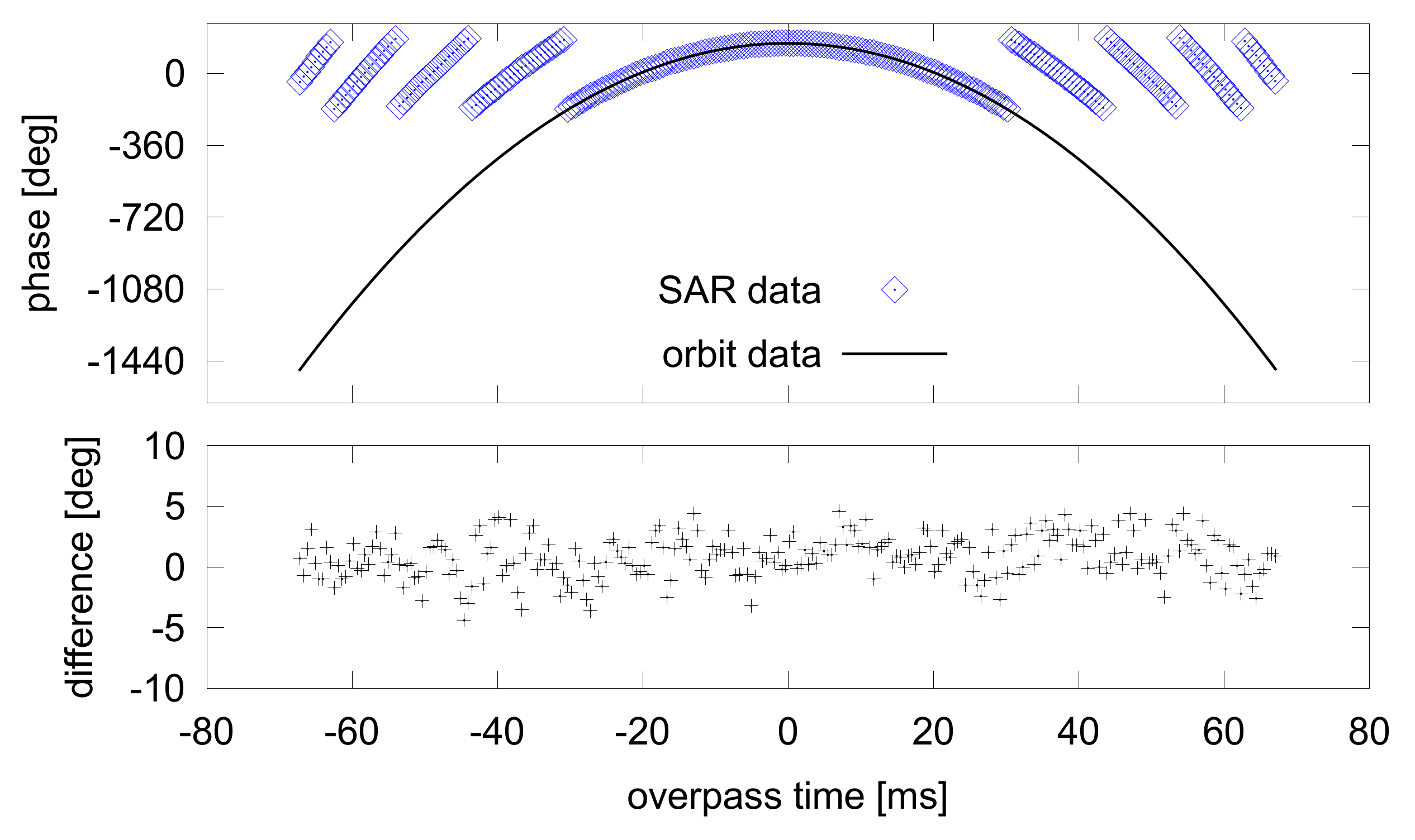
Figure 4.
Amplitude of azimuth compressed data for different orbit data; each circle represents an individual range line. A complex interpolation is applied to improve the resolution (lines). In case of precise geometry information (precise orbit data), the maximum matches at the origin with a low remaining azimuth offset of 7 cm. Using a predicted orbit, an azimuth offset of about 5 m occurs due to more inaccurate positions and timestamps of the spacecraft.
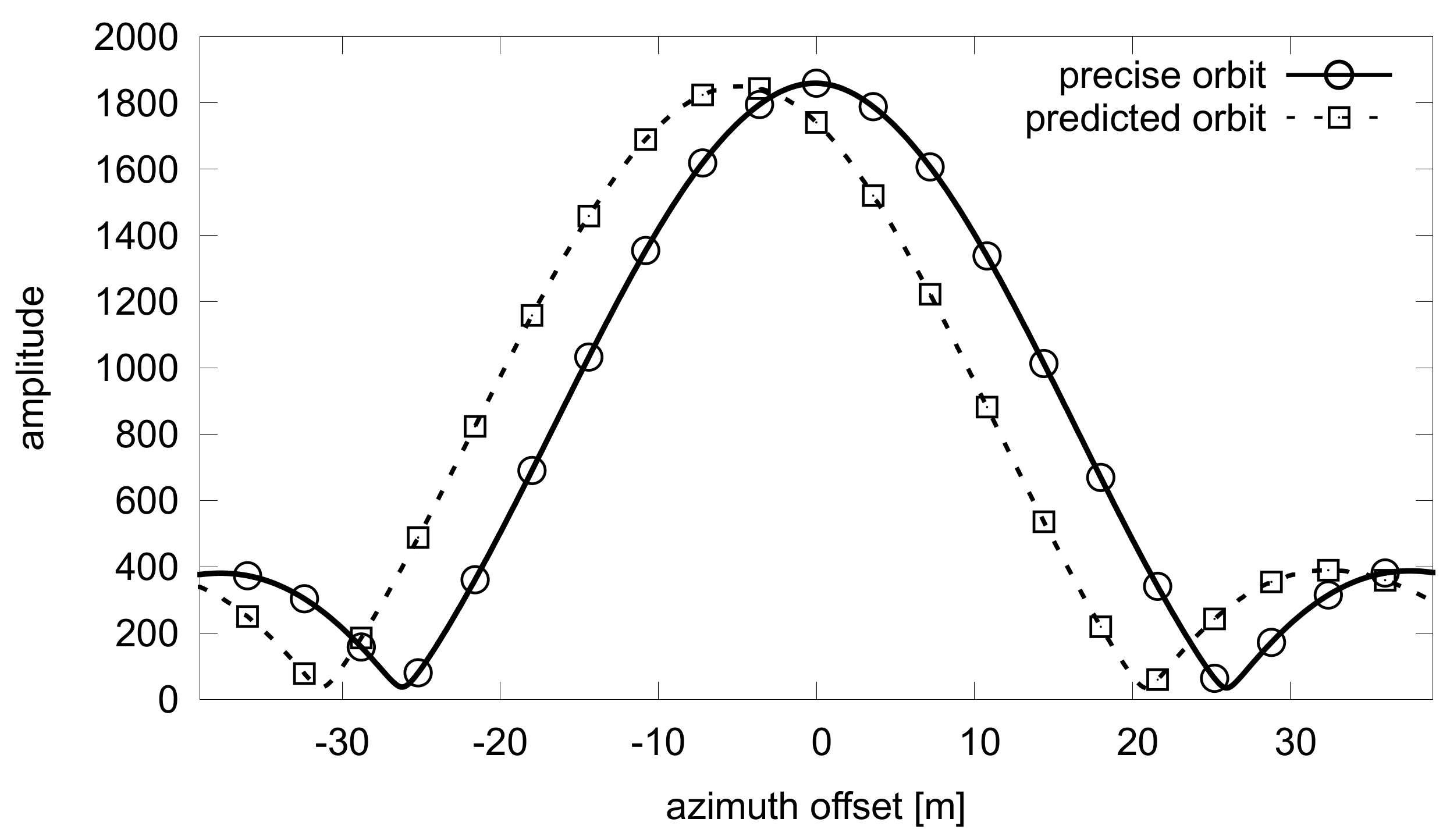
Figure 5.
Height corrected zenith path delay from the permanent GNSS network EUREF for two stations (OBE4: Oberpfaffenhofen, Germany; PFA2: Bregenz, Austria) nearby the DLR calibration field covering an observation period of one month for S-1A acquisitions during summer 2015 (a) and for S-1B early in 2017 (b).
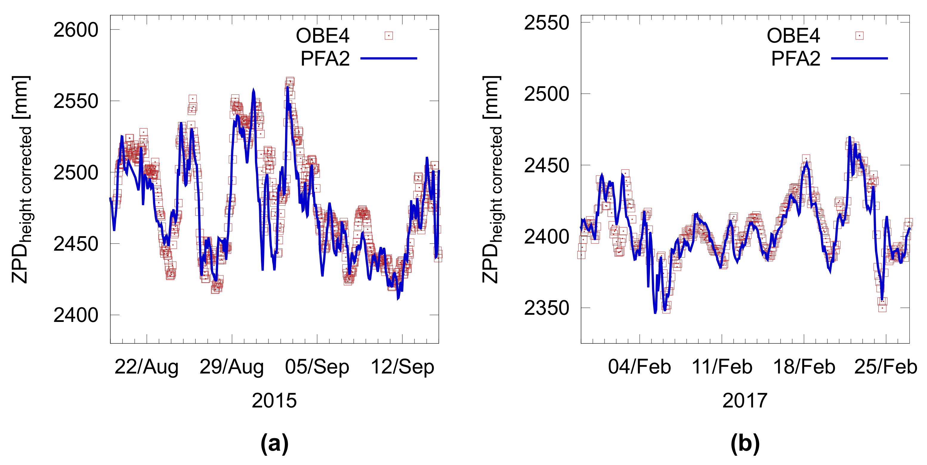
Figure 6.
Range offset derived from corner reflector responses for S-1A (a) and S-1B (b) obtained using both product types: L0 products (blue) and L1 products (black).
Figure 6.
Range offset derived from corner reflector responses for S-1A (a) and S-1B (b) obtained using both product types: L0 products (blue) and L1 products (black).
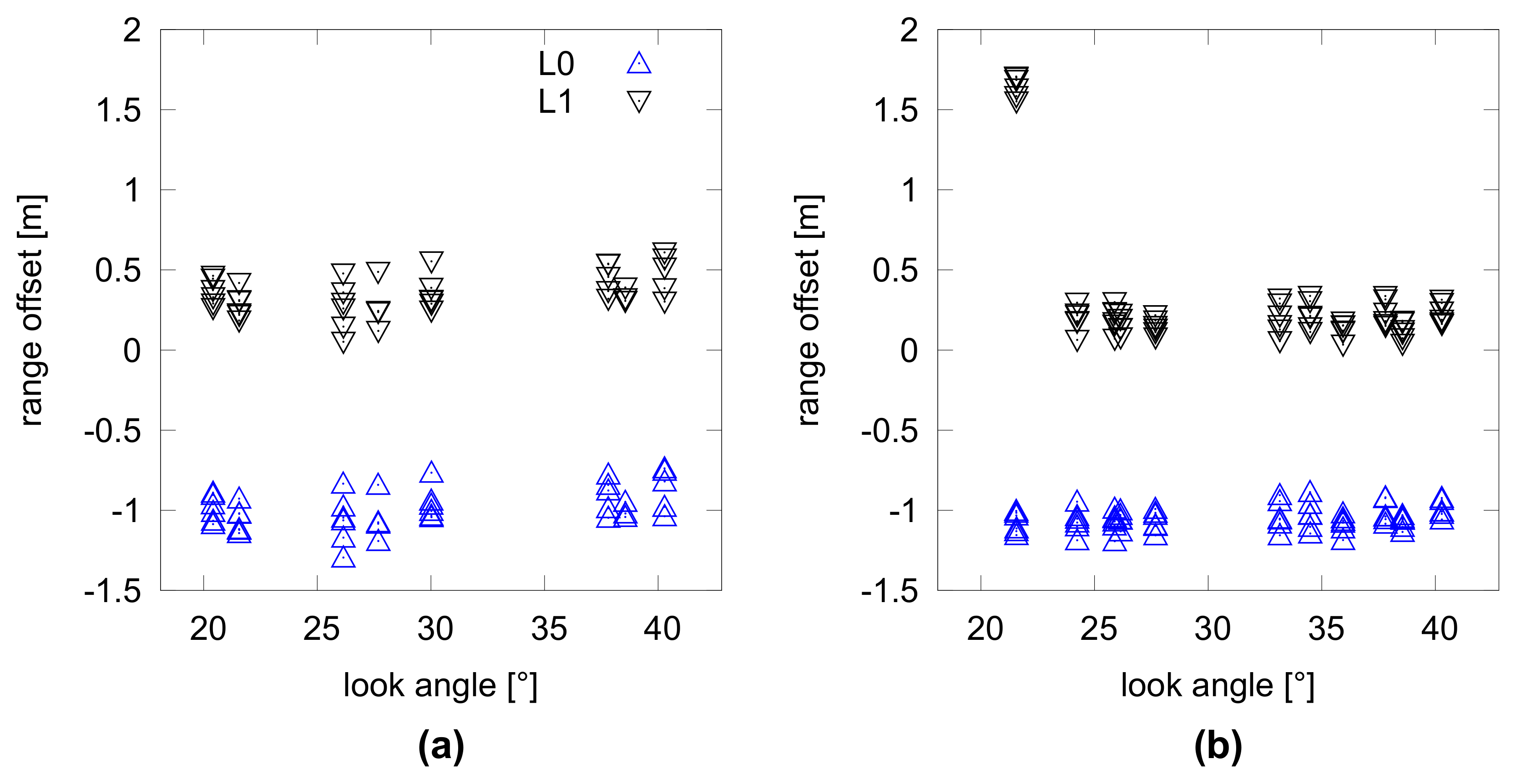
Figure 7.
Azimuth offset derived from corner reflector responses for S-1A (a) and S-1B (b) obtained using both product types: L0 products (blue) and L1 products (black).
Figure 7.
Azimuth offset derived from corner reflector responses for S-1A (a) and S-1B (b) obtained using both product types: L0 products (blue) and L1 products (black).

Table 1.
Stripmap mode observation period over the DLR calibration site.
| Satellite | S-1A | S-1B |
|---|---|---|
| Observation Period | August–October 2015 | December 2016–February 2017 |
| S1-ASC | S1-DES | |
| S1-DES | S2-ASC | |
| Acquired Beams/ | S3-ASC | S3-DES |
| Orbit Direction | S3-DES | S4-ASC |
| S6-ASC | S5-DES | |
| S6-DES | S6-ASC |
Table 2.
Geometric accuracy for DLR’s three remote controlled corner reflectors (CR) for each dimension (x, y, z) and the absolute position error .
Table 2.
Geometric accuracy for DLR’s three remote controlled corner reflectors (CR) for each dimension (x, y, z) and the absolute position error .
| Target | Mean dx (cm) | Mean dy (cm) | Mean dz (cm) | (cm) |
|---|---|---|---|---|
| CR-1 | 0.5 | −0.7 | −0.5 | 2.5 |
| CR-2 | 1.0 | 0.2 | −0.5 | 2.4 |
| CR-3 | 1.4 | −0.6 | −0.7 | 2.9 |
Table 3.
Mean value and standard deviation () for estimated range and azimuth offset using L0 data with the proposed method and L1 products for both S-1A and S-1B. Note that, for the S-1B range offset using L1 products, the outliers from Stripmap beam S1 are excluded (*).
Table 3.
Mean value and standard deviation () for estimated range and azimuth offset using L0 data with the proposed method and L1 products for both S-1A and S-1B. Note that, for the S-1B range offset using L1 products, the outliers from Stripmap beam S1 are excluded (*).
| S-1A | S-1B | |
|---|---|---|
| L0 products—Range offset (m) | ||
| L1 products—Range offset (m) | () * | |
| L0 products—Azimuth offset (m) | ||
| L1 products—Azimuth offset (m) |
© 2018 by the authors. Licensee MDPI, Basel, Switzerland. This article is an open access article distributed under the terms and conditions of the Creative Commons Attribution (CC BY) license (http://creativecommons.org/licenses/by/4.0/).
Share and Cite
MDPI and ACS Style
Schmidt, K.; Reimann, J.; Tous Ramon, N.; Schwerdt, M. Geometric Accuracy of Sentinel-1A and 1B Derived from SAR Raw Data with GPS Surveyed Corner Reflector Positions. Remote Sens. 2018, 10, 523. https://doi.org/10.3390/rs10040523
AMA Style
Schmidt K, Reimann J, Tous Ramon N, Schwerdt M. Geometric Accuracy of Sentinel-1A and 1B Derived from SAR Raw Data with GPS Surveyed Corner Reflector Positions. Remote Sensing. 2018; 10(4):523. https://doi.org/10.3390/rs10040523
Chicago/Turabian StyleSchmidt, Kersten, Jens Reimann, Núria Tous Ramon, and Marco Schwerdt. 2018. "Geometric Accuracy of Sentinel-1A and 1B Derived from SAR Raw Data with GPS Surveyed Corner Reflector Positions" Remote Sensing 10, no. 4: 523. https://doi.org/10.3390/rs10040523
Note that from the first issue of 2016, this journal uses article numbers instead of page numbers. See further details here.