Monitoring Quarry Area with Landsat Long Time-Series for Socioeconomic Study
by
Haoteng Zhao
1,2, 
Yong Ma
1, 
Fu Chen
1,*,
Jianbo Liu
1,
Liyuan Jiang
1,2,
Wutao Yao
1,2 and
Jin Yang
1 1
Institute of Remote Sensing and Digital Earth, Chinese Academy of Sciences, Beijing 100094, China
2
University of Chinese Academy of Sciences, Beijing 100049, China
*
Author to whom correspondence should be addressed.
Remote Sens. 2018, 10(4), 517; https://doi.org/10.3390/rs10040517
Submission received: 8 January 2018
/
Revised: 6 March 2018
/
Accepted: 20 March 2018
/
Published: 26 March 2018
(This article belongs to the Special Issue Analysis of Multi-temporal Remote Sensing Images)
Abstract
:Quarry sites result from human activity, which includes the removal of original vegetation and the overlying soil to dig out stones for building use. Therefore, the dynamics of the quarry area provide a unique view of human mining activities. Actually, the topographic changes caused by mining activities are also a result of the development of the local economy. Thus, monitoring the quarry area can provide information about the policies of the economy and environmental protection. In this paper, we developed a combined method of machine learning classification and quarry region analysis to estimate the quarry area in a quarry region near Beijing. A temporal smoothing based on the classification results of all years was applied in post-processing to remove outliers and obtain gently changing sequences along the monitoring term. The method was applied to Landsat images to derive a quarry distribution map and quarry area time series from 1984 to 2017, revealing significant inter-annual variability. The time series revealed a five-stage development of the quarry area with different growth patterns. As the study region lies on two jurisdictions—Tianjin and Hebei—a comparison of the quarry area changes in the two jurisdictions was applied, which revealed that the different policies in the two regions could impose different impacts on the development of a quarry area. An analysis concerning the relationship between quarry area and gross regional product (GRP) was performed to explore the potential application on socioeconomic studies, and we found a strong positive correlation between quarry area and GRP in Langfang City, Hebei Province. These results demonstrate the potential benefit of annual monitoring over the long-term for socioeconomic studies, which can be used for mining decision making.

1. Introduction
After the 1980s in China, especially in Beijing, there was a rapid expansion in economic growth with cities and urban areas consuming a huge amount of building materials. Between 1982 and 2015, the population in Beijing increased from 9.23 million to 21.71 million with an annual increase of 2.6%. In the same period, the built-up area in Beijing grew from 303.91 km2 to 1401.01 km2 (http://data.stats.gov.cn/english/easyquery.htm?cn=E0103). The growing population, the urban sprawl, and the improvement of infrastructures during the past three decades in Beijing have meant that quarries have progressively exploited the surrounding mountains. More specifically, quarries in Langfang City of Hebei Province went through an enormous expansion because of the great development of the major cities around this region. Metropolises such as Beijing and Tianjin experienced a wide upsurge in building construction and the materials of these buildings came mainly from the nearby quarries considering the transportation fees. Overall, the continuous urban sprawl has given rise to long-lasting quarry activity in the nearby mountains. Quarries contribute a great part to local government revenue, which pushes the industry of building material to a leading position in Hebei‘s economy. Quarries developed in a highly unsupervised manner during its early age, and its change was mainly subject to supply and demand at that time. With rapidly increasing house prices and in the absence of sound supervision from local governments, quarry areas may undergo continuous growth. However, with the intervention from local government, the direction and magnitude of its dynamics may change dramatically due to changes in economic policy and environmental initiatives. Therefore, monitoring quarry-rich regions at multi-temporal and high spatial resolution is important for local governments to gain information that is needed for the policies of economic and environmental protection.
Surface mining activities range from large open-cast coal and base metal mines to much smaller aggregate (rock, gravel, and sand), industrial minerals (potash, clay), and building material (granite, stone and marble) quarries [1]. Mining operations are done in a place called a quarry or quarry site. A successful monitoring approach for evaluating surface mining processes and their dynamics on a regional scale requires observations with frequent temporal coverage over a long time to differentiate natural changes from those associated with human activities. To meet such challenges, accurate and up-to-date information is needed. Since the 1970s, analog aerial photographs have been used to map spatial changes in mined areas [2]. Today, remote sensing with its capability of establishing calibrated observations over decadal-scale time periods and at sufficiently high spatial resolution (≤30 m) can provide this information to achieve better insight into quarry dynamics. Several local and regional studies have focused on the dynamics of quarries using a variety of remotely-sensed datasets with various spatial and temporal resolutions [1,3,4,5,6,7,8,9,10]. The findings from these studies have demonstrated the ability of remote sensing to detect and analyze the magnitude and spatial changes of natural environments as a result of mining activities [3,4]. However, most prior remote sensing studies focusing on quarry area changes have been temporally limited, relying on the comparison of imagery from two to three time slices (e.g., [1,5,6,9,10]). Studies [5,6] with high spatial resolution images (<5 m) usually focused on rather short time scales, ranging from several months to a couple of years due to the limited extent and availability of very high-resolution imagery, while other analyses typically span a couple of decades. On the other hand, several studies have turned to multi-temporal analyses either with multi-sourced data [8] or a single source of data (Landsat) [7]. Moreover, the diversity of data sources and the acquisition timing has resulted in limited comparability among the different studies. In this study, we used Landsat data series over a long time and with sufficient observations to fully investigate quarry dynamics. Unlike [7,8], we aimed to obtain an annual result of quarry area, trying to further investigate the relationship between quarry dynamics and local economy using the acquired quarry area series.
Since the entire Landsat archive is freely provided by USGS, it becomes viable to exploit this valuable and consistent data source to access multi-scaled land surface dynamics in most regions. Recently, with increasing computation capacities and novel processing techniques, more and more studies focusing on monitoring high-resolution land cover changes have shifted focus toward a high frequency multi-temporal analysis using the entire Landsat archive, with over 40 years of continuous acquisitions. Examples include mostly forestry applications. For example, Kennedy, Cohen, and Schroeder [11] applied a trajectory-based change detection method to a stack of Landsat images from 1984 to 2004 to monitor forest disturbance dynamics; Hansen et al. [12] mapped global forest loss and gain from 2000 to 2012 based on Landsat data; Rosenau, Scheinert, and Dietrich [13] monitored glacial flow velocities both at decadal and seasonal time scales using Landsat imagery; and Macander et al. [14] mapped snow persistence for Northwest Alaska using Landsat images from 1985 to 2011. These studies are predominantly based on the analysis of multi-spectral indices (MSI) or the original spectral bands. In Fraser et al. [15], robust linear trend analysis of temporal Landsat Tasseled Cap (TC) index time-series was proposed and applied in different studies of land changes, such as post-fire forest recovery [16], lake dynamics [17], and the land cover change classification [18]. Recently, Google Earth Engine [19] has greatly facilitated the temporal applications of the Landsat archive with its powerful cloud computing ability, such as the monitoring of urban boundaries [20] and woody vegetation clearing [21].
We noticed that quarry changes might have a potential relationship with the regional economy for it is a result of human activities and economic development. However, with the scarce observations so far, the potentially strong relationship between quarry area and economic parameters have not been sufficiently analyzed. Few studies have examined the correlation between quarry area and GDP or gross regional product (GRP), whereas a large number of statistical studies have demonstrated that there is a positive correlation between GDP and remotely sensed nighttime light data captured by Operational Linescan System (OLS) of the US Defense Meteorological Satellite Program (DMSP) [22,23,24,25]. This research indicates that it is feasible to use nighttime lights to estimate GDP or GRP. Therefore, we were inspired to research whether quarry area captured by Landsat satellites has a positive correlation with GDP or GRP and investigate the possibility of using daytime remote sensing data for socioeconomic study.
In this study, we first examined the areal expansion of aggregate quarries over 34 years in the study region in Northern China, using remote sensing techniques. Due to the small extension of quarries in one year, we chose a single imagery captured by the Landsat 5 or Landsat 8 satellite for each year between 1984 and 2017. We then applied a modified random forest classification for quarry range extraction and analyzed quarry dynamics in the study region. The studied regions governed by the Hebei and Tianjin governments allow us to compare different quarry dynamics responding to different policies in these two places. Our analysis aims to detect decadal-scale changes in the quarry sites, as well as the relationship between quarry area and socioeconomic parameters. We try to demonstrate in this study that quarry area extracted from remote sensing data can be used to sense society changes, for many land cover changes should be a result of human activities and social development.
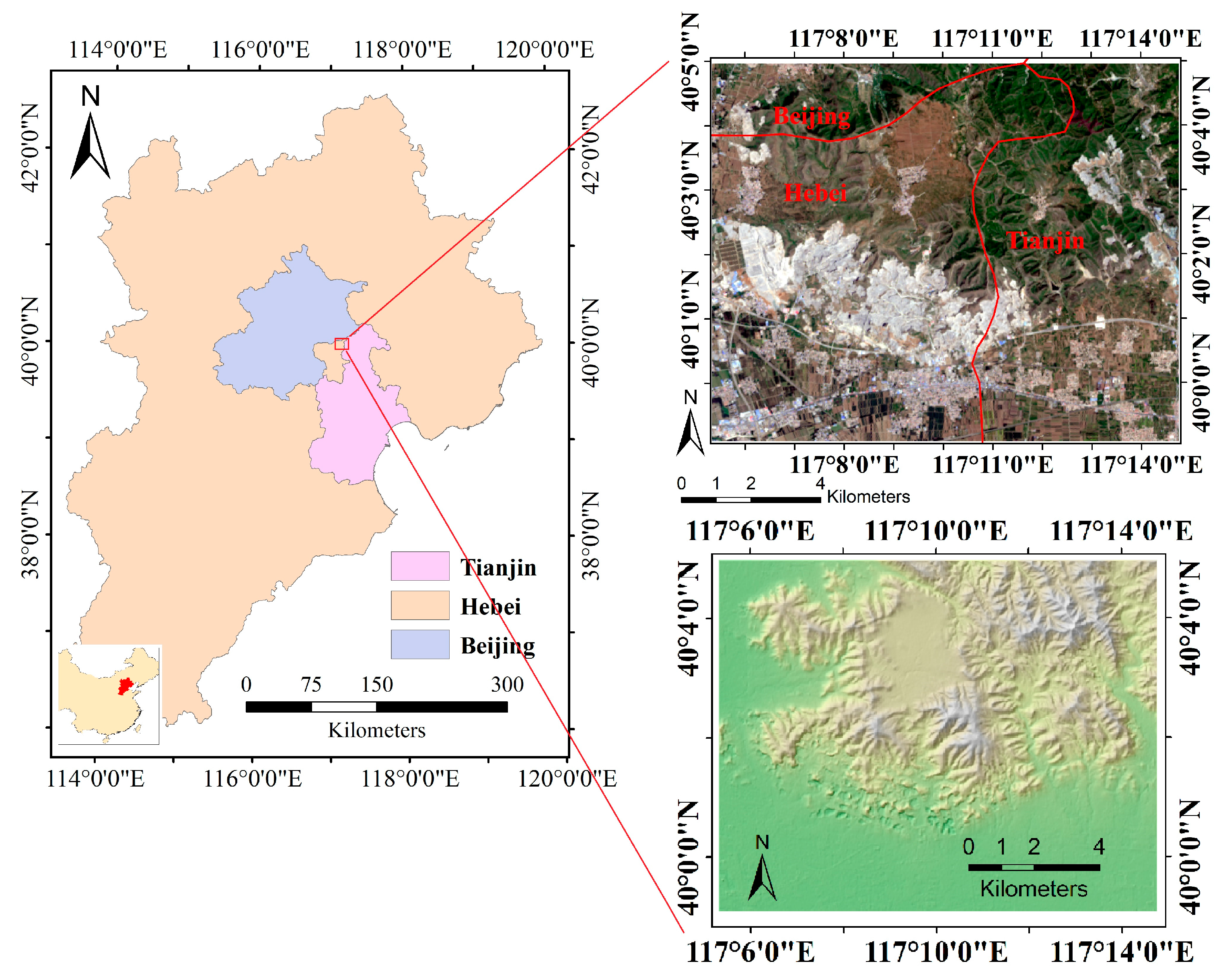
2. Study Area
The study area we chose is part of the middle range of the Yanshan Mountains, located in the northeast of Langfang City, Hebei Province, China, where it has been exploited for aggregate since the 1980s. The study area is situated on the border of Beijing, Tianjin, and Hebei, east of Beijing city (Figure 1). Its location is in the north of China between latitudes 39°59′ and 40°5′N and longitudes 117°5′ and 117°14′E and covers an area of about 145 km2 (Figure 1). The highest altitude in this area is 527 m above sea level and the lowest is 4 m.
There is a large amount of high-quality dolomite ore, limestone, shale, and other minerals under the hills in the study area. In the early 1980s, some locals had exploited these minerals for profit. With the development of urbanization in the surrounding region, a large amount of stone building materials have been required for a growing number of construction projects in the cities every year. Considering the cost of transportation, most stone building materials such as aggregates and cement come from quarry sites around the cities. The growing rock market triggered the rapid extraction of rocks from these hills. With the rise in housing prices, the price of stone in mining enterprises soared, resulting in mining activity that can be seen everywhere in the hills inside the study area. We choose this region as the study area because it contains quarry sites in both Langfang and Tianjin. This facilitates the comparison of quarry dynamics in the two regions, and the study period can effectively represent the quarry changes both in the early period when local people dominated the exploitation activity and in the later period when the government has managed the production and recovery in the quarry sites. The changes in the study area also reflect the many socioeconomic parameters and some big events that happened around this region.
3. Materials and Methods
3.1. Data
While there are numerous satellites orbiting the globe with a multitude of instruments onboard that explore various bandwidths in the electromagnetic spectrum, Landsat-based images are ideally suited for surface feature analyses because of the long history of earth observation and rich bands with ample spectral information [26]. Note that Landsat 5 Thematic Mapper (TM) operational imaging ended in November 2011 [27]; subsequently, Landsat 8 was launched in February 2013 [28]. Therefore, only Landsat 7 imagery with missing data are available for 2012 due to the failure of the Enhanced Thematic Mapper Plus (ETM+) Scan Line Corrector (SLC) on Landsat 7 post-2003.
In this study, an annual observation is enough for tracking quarry areal extents because the processes that drive quarry area growth or decline are slow enough to be captured well with an annual repeat frequency. Thanks to the high temporal frequency of capturing images, we can easily find ideal annual observations with low cloud coverage from 1984 to present. Eventually, 33 Landsat 5 (TM) and Landsat 8 (Operational Land Imager—OLI) images were picked from the US Geological Survey’s (USGS) EarthExplorer platform (https://earthexplorer.usgs.gov), representing years from 1984 to 2017 (except 2012), and WRS Paths 122 to 123 and Rows 32. All scenes were ordered as surface reflectance (SR) data. Landsat 5 SR data provided by USGS are generated using the atmospheric correction chain called Landsat Ecosystem Disturbance Adaptive Processing System (LEDAPS) [29]. In 2010, USGS Earth Resources Observation and Science Center (EROS) released on-demand LEDAPS processing for generating SR products for the entire Landsat 5 archives (http://espa.cr.usgs.gov). On the other hand, Landsat 8 SR data are generated from the Landsat Surface Reflectance Code (LaSRC) [30]. Currently, both Landsat 5 and Landsat 8 SR data can be ordered using EarthExplorer. Because of the SLC failure of Landsat 7, we chose not to pick data for 2012 in order to avoid the influence of the missing scan line data in ETM+ images. The images from TM and OLI sensors have a common spatial resolution (30 m) and (six) overlapping spectral bands: blue, green, red, near-infrared (NIR), shortwave infrared 1 (SWIR1), and shortwave infrared 2 (SWIR2). All common spectral bands were used for analysis while the remaining bands were excluded from further processing. Images from the first Landsat sensor generation (Multispectral Scanner/MSS) were not taken into consideration at this point because of their coarser spatial resolution and lower spectral fidelity. The image selection was filtered to acquisition dates in May as we observed that Landsat images of the study area always had no or very little cloud in May among these years. Finally, we got 33 scenes with a cloud coverage near to zero in the study area. Detailed image ID and acquired dates are shown in Appendix A.
For our analysis, we used GRP data of Langfang City from 1990 to 2016. All data came from the Hebei Economic Yearbook [31], which contains the annual economic development of Hebei Province as recorded by the Statistics Bureau of Hebei Province.
3.2. Methods
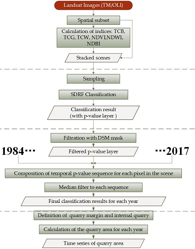
The method developed in this study follows a workflow of automatic image clipping and indices calculating, and subsequent classification and calculation of the quarry area based on a modified classification and quarry region analysis. The methodological framework is presented in Figure 2 and described in the following four subsections: pre-processing (Section 3.2.1), classification (Section 3.2.2), post-processing (Section 3.2.3), and calculation of quarry area (Section 3.2.4).
3.2.1. Pre-Processing
After being downloaded from USGS, all images were clipped into the study area. Then, we calculated several multispectral indices for each scene, serving as proxies for different land surface properties. We included the Landsat specific Tasseled Cap indices of brightness (TCB), greenness (TCG), and wetness (TCW) [32,33,34], as well as other general indices, such as the Normalized Difference Vegetation Index (NDVI) [35], the Normalized Difference Water Index (NDWI) [36], and the Normalized Difference Building Index (NDBI) [37]. They were chosen to reflect a variety of surface characteristics such as vegetation status, surface moisture, or buildings. The TC indices were calculated with the sensor-specific formulas for reflectance data. The calculation was performed using the following equations:
Then, the six calculated index layers were stacked together with the six original bands to get a 12-band scene for each year.
3.2.2. Classification
We first applied a supervised machine learning classification approach, which separated the image into two target classes: quarry class and non-quarry class. Random forest [38] (RF) has been established as one of the most accurate and widely used algorithms [39,40,41,42] for remote sensing and other classification applications. One of its advantages is that it produces an estimation of classification accuracy based on out-of-bag cross-validation (OOB-CV) [43,44,45]. However, OOB-CV strongly overestimates model accuracy when classifying remote sensing imagery using training areas with several pixels, which was recently demonstrated in [46]. The authors of [46] think the reason is that pixels in a training patch are not independent—they have a strong spectral similarity—whereas the OOB-CV takes all samples as being independent. To deal with the problem, a modification of the RF algorithm, splitting the training patches instead of the pixels that compose them, is proposed in [46] and implemented in the R package called SDRF (Spatial Dependence Random Forest). For the classification process, we used the modified random forest function in the SDRF package. In this function, there are two important parameters that should be controlled to acquire a better classification result: ntree (number of trees to grow), and mtry (number of variables randomly sampled as candidates at each split). Since the random forest classifier is computationally efficient and does not overfit, the number of trees can be as large as possible [47]. However, the classification no longer improved as the number of trees increased above a threshold, as demonstrated in some studies investigating the sensitivity of the RF classifier to the number of trees [42,48]. A default value of ntree for remote sensing imagery classification is 500. Higher mtry will result in stronger individual decision trees but with an enhanced correlation between trees the model accuracy is reduced [49]. Usually, a square root of the total number of variables is used in the classification task.
Training Sampling
We selected 20~50 training sample areas within and in close proximity to our study sites with respect to a set of remote sensing imagery with higher resolution, which mainly came from Google Earth. The ground truth selection process is based on a stratified manual sampling. Since the non-quarry class can have a variety of different surface conditions, we increased its sample size to attribute for this variety. We assumed that quarry range changes slightly over several years and its change limits to its boundary. Therefore, once a sample is identified as an inside part of the quarry according to high-resolution images, we can assume this sample remains unchanged in several near years unless it shows an extensive spectral change on these years’ images. The Landsat data and in situ data, as well as high-resolution images, were used for determining suitable locations of the manually selected and determined ground truth locations.
Classification Method Details
The six common spectral bands (blue, green, red, NIR, SWIR1, and SWIR2), as well as the six calculated indices (TCB, TCG, TCW, NDVI, NDBI, NDMI), were used as input features for the pixel-based classification process. The SDRF classification model was trained for each image in every year using the respective training samples. The two parameters ntree and mtry were determined with a test based on the modified out-of-bag (M-OOB) accuracy in this study and we found that the number of 500 for ntree and 4 for mtry worked well for the classification task. As the quarry area covered only a small fraction of the study area before 1995, we used the class weights for the models before 1995 according to the prior of the sample areas.
The classification output contains a hard classification output with the two pre-defined classes (Table 1). This is an ensemble result voted by all decision trees in the RF classifier. The random forest can also output a ratio result for each class, which is calculated as the proportion of trees voting for one class against all votes. Each ratio result is output as a confidence layer for each class, which contains the classification probability (confidence index) of each class in a range from 0 to 1. The SDRF-internal M-OOB accuracy, Cohen’s Kappa, and area under the ROC curve (AUC) were used for quality assessment of the classification.
3.2.3. Post-Processing
The output from the random forest is a per-pixel classification with two classes. The per-pixel results tend to be noisy due primarily to the effects of pixel-scale misclassification. These effects include couples of pixels among vegetation area where naturally bare stones are misclassified as quarry. There are also some speckles in the classification results, which is common to many per-pixel classification results. Thus, a post-classification editing step is necessary.
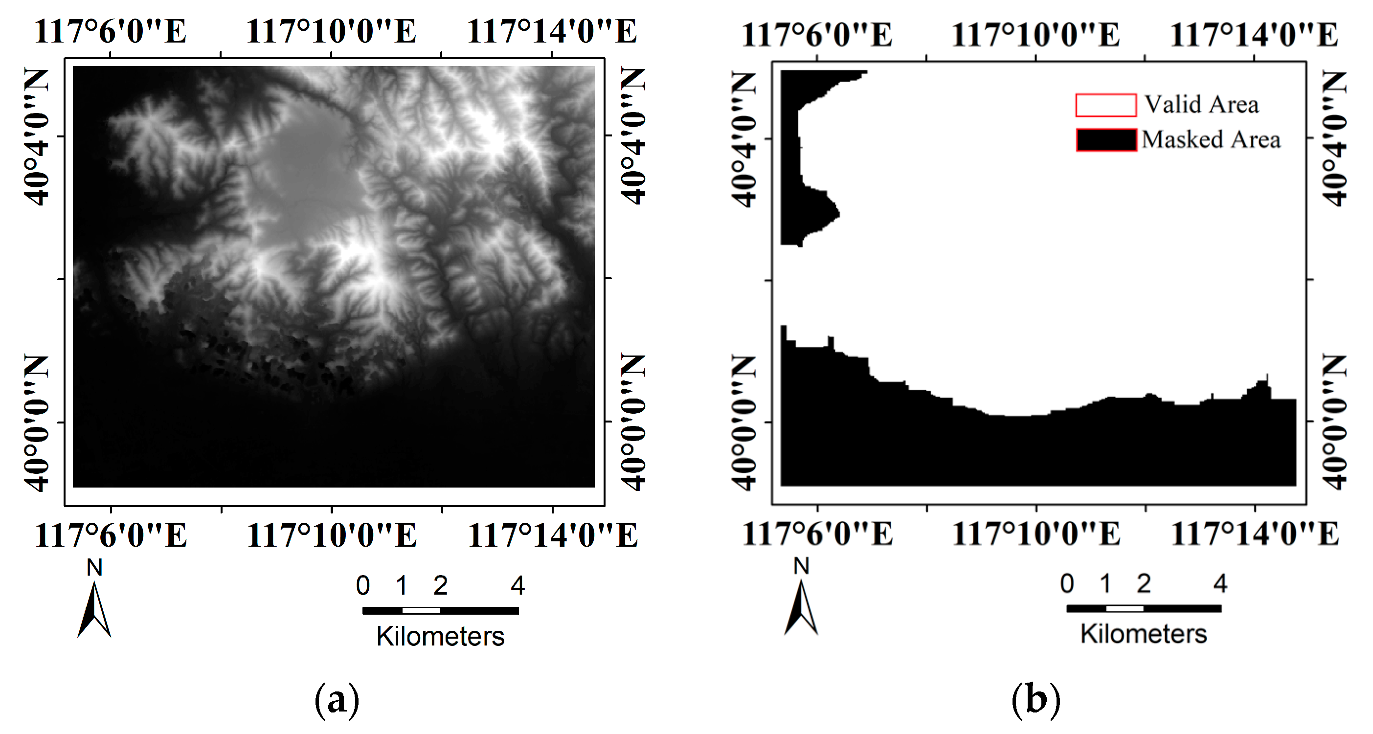
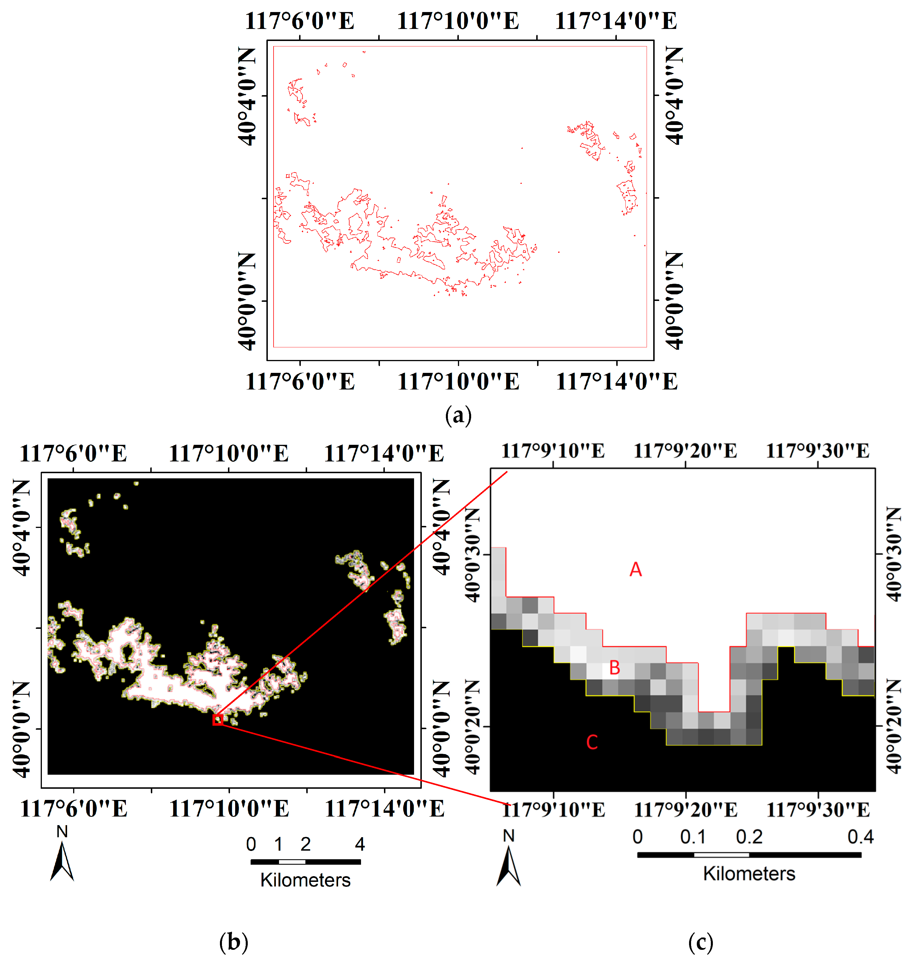
The presence of bright topographic features dominated by cement and stones poses a challenge when trying to extract quarry location. For example, cement ground, cement roads, and the depositories for raw rock materials in the flat terrain can be mistaken by the analysis algorithm as quarry sites as they present a very similar ground feature because of their similar surface materials. Thus, we need to introduce some degree of filtering that would eliminate anomalous pixels from the quarry pixels. For example, quarry sites only exist near or on hill slopes where the altitude is higher than other flat terrain. Therefore, we decided to process the classification result images with an altitude mask. We obtained the altitude mask from the ALOS DSM data by taking an area higher than 50 m as a valid field and then dilating this field by 9 pixels in order to cover quarry hollows at the foot of the hills. Figure 3 illustrates the altitude mask we processed from DSM image. Only quarry pixels inside the valid area were considered as true quarry area.
Temporal Smoothing
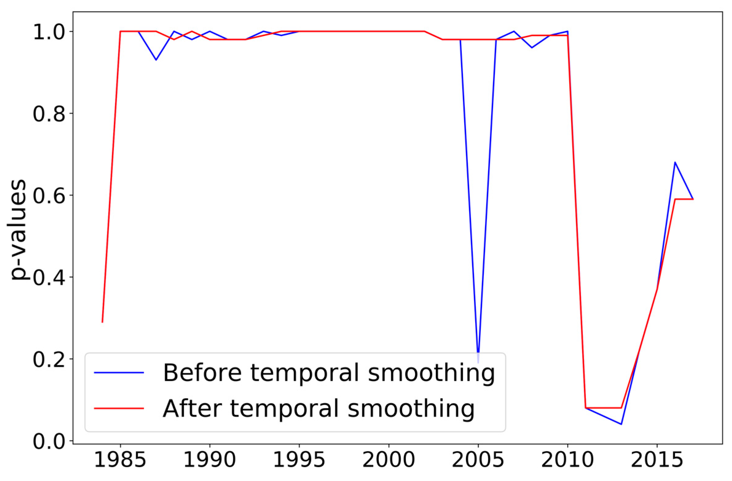
After all scenes are processed using the above steps, we applied a temporal smoothing to exclude some non-quarry pixels in the quarry class, such as dusty land caused by wind around the quarry in certain years and also to obtain a consistent change result. Once other classes are changed to quarry (always with the removal of vegetation and surface soil), it will remain as quarry for deep exploration of stones for the following years. For the reverse situation, once a quarry changes to other classes, whether naturally or artificially, it would not change back to a quarry in a short time because it is obviously forgotten or protected by humans. Based on this, it is safe to assume that outliers in the temporal sequence of confidence index is very possible a misclassified one. For each class, we first composed a confidence sequence for each pixel by putting together the confidence index of each year in order. Then, we applied a median filter to the sequences in order to remove outliers and obtain gently changing sequences along the observation period. An example of this method is expressed in Figure 4 where the lines indicate the confidence index of the quarry class during the monitoring period. Obviously, an outlier in 2005 is successfully removed using the temporal smoothing strategy.
3.2.4. Calculation of Quarry Area
During the final step, we calculated the areal extent of quarries in the study area. We noted that unlike other naturally occurring changes, such as land becoming a lake, quarries are exploited by humans in a short time, which means we cannot distinguish a transitional state of the land between quarry and other land-cover types. Therefore, it is reasonable that we obtained a per-pixel classification with just two classes. However, in the quarry margins, quarry expansion tends to occur on a sub-pixel scale (<30 m), resulting in mixed pixels in these areas. In order to obtain an accurate area result, we calculated the area of the internal zone and margin zone in different ways.
Based on the hard classification results, edges of quarries were identified. Then, we defined two zones to obtain a sub-pixel level accuracy in the quarry area calculation. The quarry margins are defined by the edges being dilated by 1 pixel to capture the sub-pixel expansion of the quarry. To obtain the internal zone, we used the hard-classified quarry mask and applied a morphological erosion to reduce the quarry’s radius by 1 pixel to avoid the quarry margin.
The two defined zones were treated differently. The internal zone was regarded as pure pixels and its area was therefore calculated as a full quarry area. For margins, we chose a more dynamic sub-pixel analysis approach to account for its mixed pixels. Its area was represented by the classification probability (confidence index), which was assumed to be the fraction of each endmember/class and they were tested for plausibility on high-resolution imagery, as well as field measurements and observations, which were available for selected locations. These confidence indices were used as a weighing factor of quarry class within each pixel of the quarry margins. For example, a pixel in the margin zone has a confidence index of 0.705 for a quarry, representing 70.5% of the 900 m2 per- pixel; hence, 634.5 m2 is calculated as quarry within this pixel. Figure 5 is an example taken from the classification result of 2002 to illustrate the calculation process.
4. Results
4.1. Classification Accuracy
The classification of two defined classes yielded a very good separation on the ground truth data of the defined classes. M-OOB and Cohen’s Kappa, as well as AUC for the quarry class, are listed in Table 2, which suggest that the classifier archived a high accuracy using the parameters defined in Section 3.2.2.
4.2. Quarry Time Series
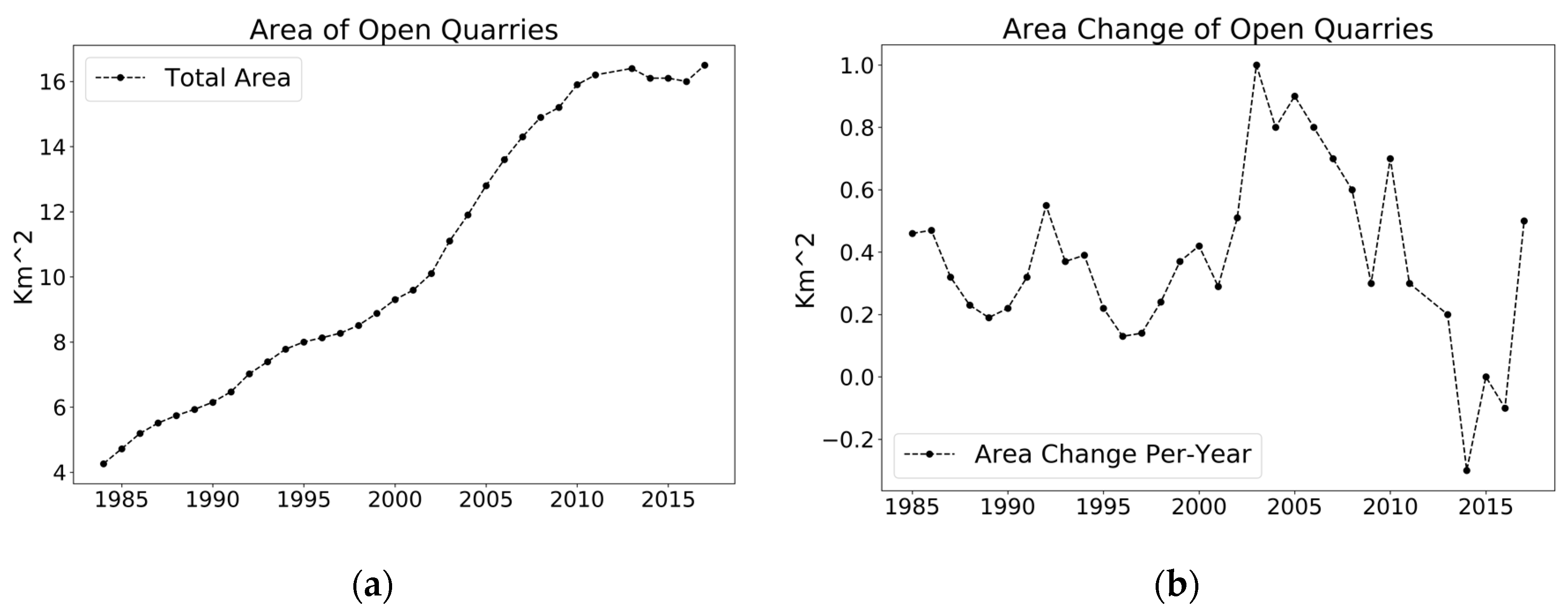
During the final step, the annual areal extent of the quarry was calculated. The quarry time series was produced after passing all images through the workflow that we described earlier spanning the period from 1984 to 2017, i.e., about 33 years of coverage. The image series had a gap in 2012 and, therefore, we actually attained a 34-year time series of quarry area.
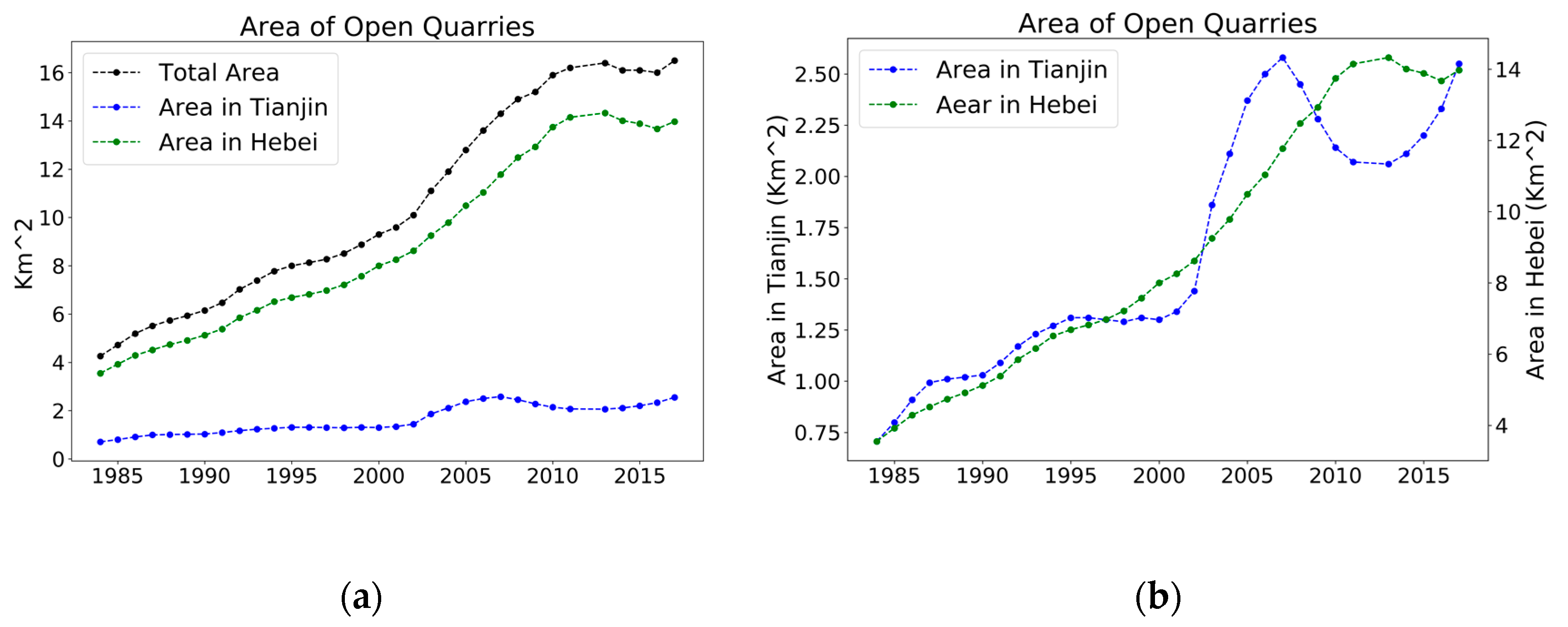
The quarry area dynamics are presented as line charts (Figure 6). The left line chart indicates the area change of the quarry during the past 34 years. Generally, the area increased before 2013 and decreased during the following 3 years. In May 2017, the quarry experienced a great expansion again. The right line chart represents its change speed at different time points, where each point means the change amount from the last year to this year. This chart insinuates different change rates at different time periods. According to its change patterns presented in the graph, five different change periods are distinguished: (1) The first period was from 1984 to 2002. In this period, the change speed kept at a low level, mainly under 0.5 km2 per year, except for the speed in 1993. The speed changed slowly, taking roughly 4–5 years to rise and fall. (2) The next period with a high change speed continued from 2002 to 2010. Its speed was greater than 0.6 km2 per year during this period, except in 2008. (3) The area then underwent a low-speed increase over the following 3 years from 2011 to 2013. (4) Its change rate dropped to negative values in the following 3 years (2013–2016), which means the quarry area went through a decline in these years. (5) Finally, from May 2016 to June 2017 sees a great areal growth in the quarry.
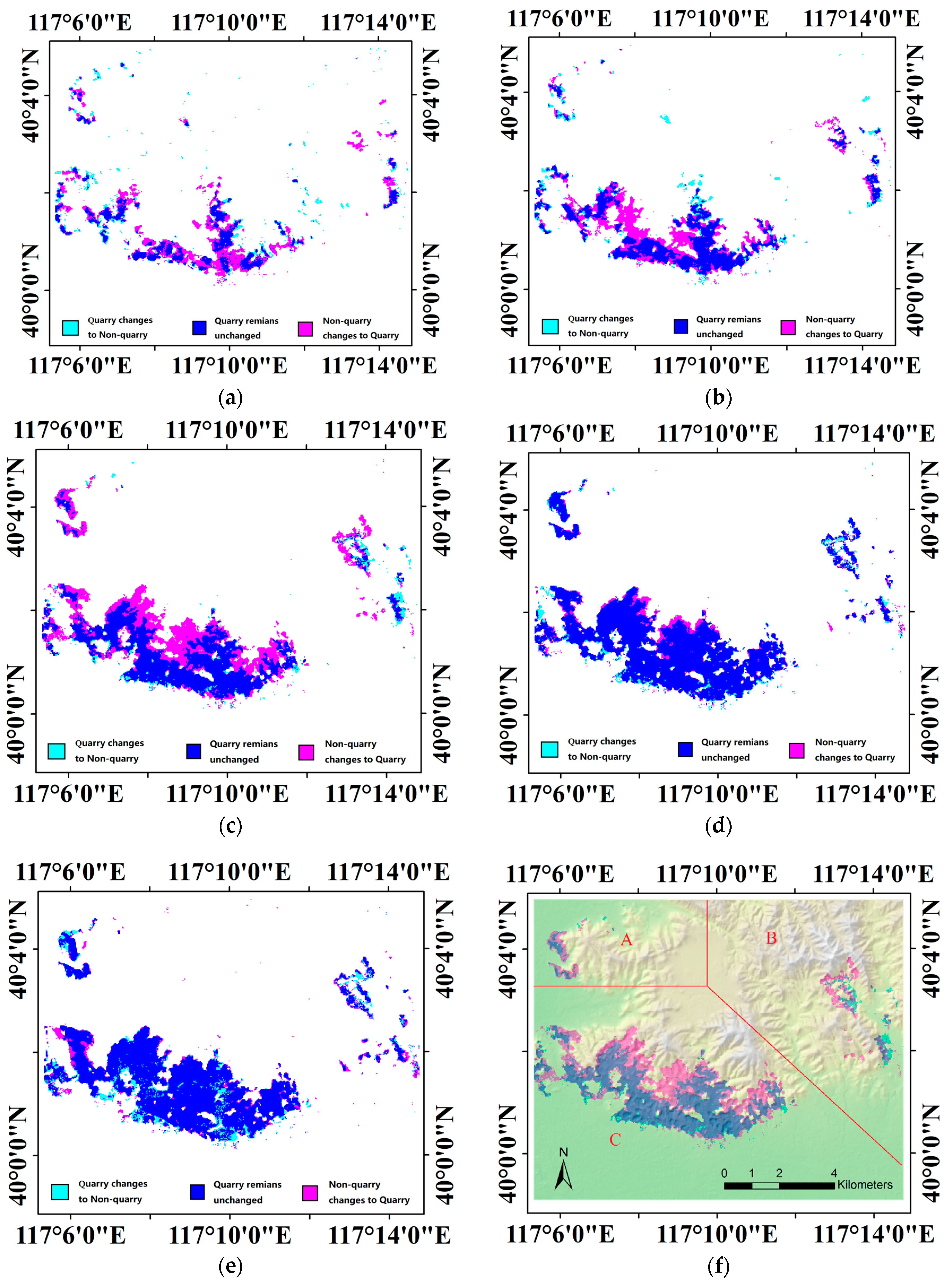
We then portrayed the changes in the quarry boundaries in each period as follows. Each map delineates the quarry ranges before and after one period. In these maps, the blue area represents unchanged quarry regions, the red area represents extended quarry regions, and the cyan area represents recovered quarry regions.
Figure 7a,b shows the two stages of change in the first period, changes between 1984 and 1992 and changes between 1992 and 2002. In the early stage of quarry activities, since 1984, quarries had a scattered distribution. In the beginning, local people were motivated to exploit the rocks for the great profits from the building materials. They extracted stones and rocks without any planning and never considered the amount of prospecting for rocks in the quarry sites. Gradually they abandoned some smaller quarries and flocked to areas where plentiful rocks suitable for construction were extracted. By 1992, the scattered quarries in places that were rich in rocks were expanded and then merged into several large quarry sites. Others sites were abandoned and then re-covered with vegetation naturally in a short time for these quarries had only been minimally exploited. Then, from 1992 to 2002 in Figure 7b, the abandoned quarries continued their recovery with vegetation cover while the large quarry area kept expanding. By 2002, the scattered quarry sites can be distinguished as three main continuous quarry regions as shown in Figure 7f: Quarry A lies in the northwest, Quarry B lies in the south, and Quarry C lies in the northeast. During the 8 years between 2002 and 2010, each of the three quarry areas expanded rapidly, which is clearly illustrated by Figure 7c. The decrease mainly happened inside Quarry C; other small decreasing parts in Quarry B were primarily on the south edge of the quarry, which was exploited earliest. From 2010 to 2013 in Figure 7d, the area increased only slightly on the north side of Quarry B. Most quarry sites remained unchanged during this period. Figure 7e demonstrates that the quarry areas in all three regions decreased between 2013 and 2016, although a small expansion occurred in Quarry C and the western part of Quarry B. We should point out that the small decreasing parts inside Quarry B were newly built buildings.
From the line charts in Figure 6, two special years are identified for presenting very different tendencies: 2008 and 2017. Between May 2007 and August 2008, the quarry area had almost no change compared to its nearby years (Figure 8a). While the main trend was still toward a decrease in the three quarry regions from June 2016 to May 2017 (Figure 8b), a very large newly exploited area in the west of Quarry B resulted in an increment in the total area. Again, the small speckles inside Quarry B were a result of intense internal rebuilding.
4.3. Uncertainties and Errors
For the classification step, we used a supervised learning method, which required a set of accurate and enriched samples. As we classified scenes of each year along the past 34 years, sampling was required for each scene and the accuracy of the results depends on the quality of the samples. Deriving operative samples from temporally adjacent samples and classifiers was demonstrated to work well in this study. However, further studies on other datasets or monitoring tasks are needed to confirm the conclusion. One more uncertainty is that when discussing the influence of social events and local policies on quarry changes, our analysis is based on the comparison of quarry areas in two jurisdictions considering some well-known events and policies. Maybe integrating some kind of quantization of the social events and policies into the analysis can present their close connection more clearly.
5. Social Discussion
Prior work has documented the feasibility of the Landsat archive for monitoring land cover changes and analyzing their dynamics in a high-resolution multi-temporal way [14]. However, studies on quarry monitoring remain temporally limited. Whether using several decades of spanned space-borne imagery or higher resolution images focusing on a short time scale, prior studies have generally relied on a comparison of imagery from two to three time slices [1,5,6,9,10]. Hence, with the focus on scarce observations so far, the socioeconomic reasons behind these quarry changes have not been thoroughly analyzed. In this study, we used a long time series data from the Landsat archive to fully investigate the annual change in the quarry area. In this section, as the annual monitored result of the quarry has been derived, we try to discuss the factors driving the quarry development from a socioeconomic viewpoint and demonstrate the potential benefits of annual monitoring in a socioeconomic study.
5.1. Comparison of Two Regions
The study area is located on the border of Beijing, Tianjin, and Hebei, making a comparison of quarry development among these areas possible. Since the development of quarry extraction is influenced deeply by human activities, it is also reasonable to discuss the quarry area extension and contraction with the different policies in the three regions, especially after the local government began to actively manage the mining.
Because the quarries in the Beijing region are actually exploited by people from Hebei Province, the study area was separated into two regions, one under the governance of Hebei Province and the other under the governance of Tianjin City, according to the boundary line between Hebei and Tianjin (Figure 9). Then, we separated the dynamics of the quarry area into two zones.
The amount of quarry area in Tianjin is quite small in the study area compared to that in Hebei Province, but is actually the biggest quarry site in Tianjin and most aggregates used in Tianjin buildings come from here. As it is so near to Hebei, its dynamics has a close relationship with that of the quarries in Hebei. Similarly, line charts are presented for a better observation of its dynamics (Figure 10). In order to compare them more easily, they are scaled in Figure 10b, which indicates that their change trajectories before 2008 were very similar. From 2008 to 2016, the change trends of the quarries in Tianjin and Hebei developed in opposite directions. The quarry area in Tianjin decreased and then increased during this period, whereas that in Hebei grew first and then decreased. They both experienced a sharp increment in 2017.
Behind these different tendencies, there are multiple socioeconomic reasons. In the early time, the government had no objection to the exploitation because of the great contribution of quarries to local revenue. Quarry activities were dominated by local people who were driven by the profits. Hence, the economy was the main factor affecting the quarries’ expansion in the two regions. However, from 2008, the government started managing quarry activities. One big reason was Beijing’s Olympic Games in 2008, which caused a forceful restraint on quarry activities, arresting the extension of the quarry area from 2007 to 2008 in total. Specifically, the Tianjin government took stricter actions on regulating its quarry since January 2008 because a serious landslide inside a quarry site of our study area in Ji County, Tianjin, resulted in the death of 12 people (http://www.gov.cn/jrzg/2008-01/14/content_857398.htm). While these actions brought about an acute recovery of the quarry area, most of the truck drivers living on the quarry sites in Tianjin had to move to nearby sites in Hebei to continue their business, thereby causing an increase in the quarry area in Hebei despite the big inhibitory factor—Beijing Olympic Games in 2008. Overall, the quarry area in Tianjin decreased and the quarry area in Hebei increased while the total quarry area stayed nearly stable. After 2011, the economic transition in China required an environmentally friendly way in which to develop the economy. Inevitably, the total area of quarries decreased before an environmentally friendly developing pattern in the mining industry was found. Additionally, around 2013, CCTV-2 Half-Hour Economy reported that many local people contracted serious respiratory diseases because of the heavy dust in the air around the quarry sites in Hebei, and pointed out that this quarry region was the largest source of air pollutants on the east side of Beijing (http://finance.sina.com.cn/china/dfjj/20130621/220515877577.shtml). After that, all these quarry sites were forced by the government to close. Therefore, this time, the miners and truck drivers moved to sites in Tianjin, causing the quarry area in Tianjin to grow again. Therefore, we can see a different tendency in quarry changes in these two regions again and an overall decreasing trend in the study area.
5.2. Relationship between Quarry Area and GRP
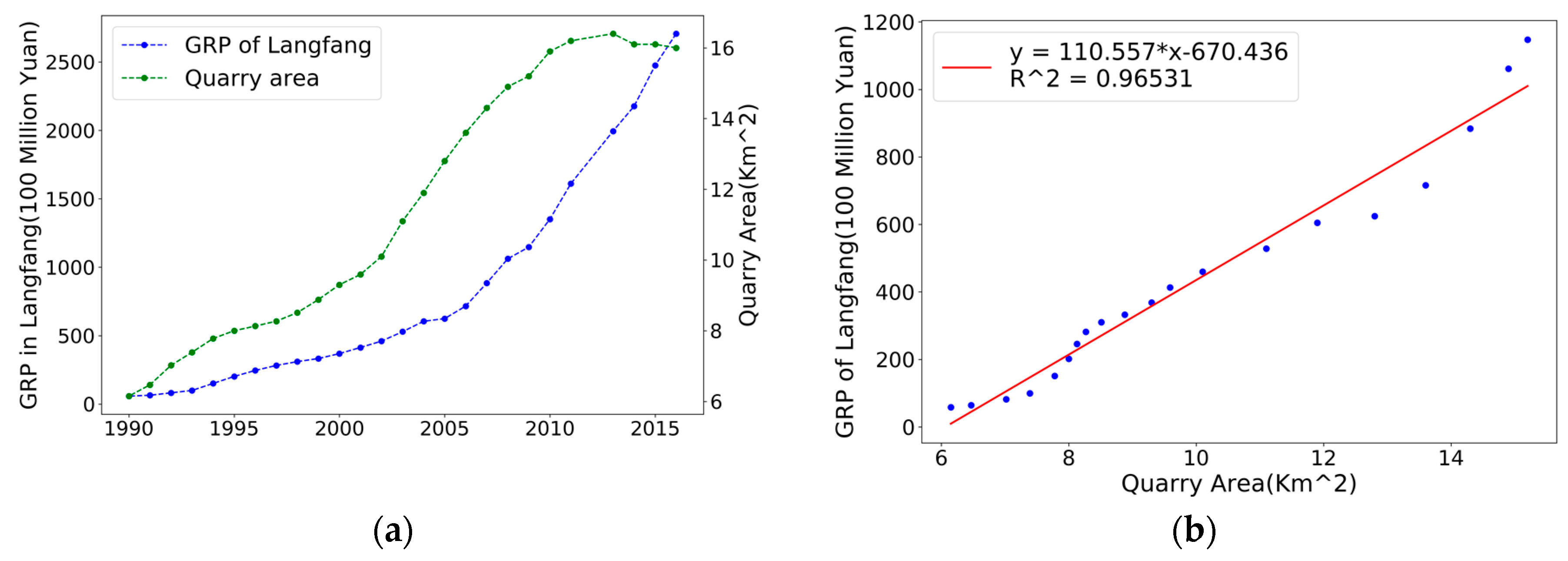
It seems natural to relate quarry area increase and economic growth because the construction industry is one of the most profitable trades in China after reform and opening up. After we have acquired the annual monitoring results of the quarry, it also becomes possible to demonstrate this potential positive relationship. In this section, we discuss the relationship between the gross regional products (GRP) and quarry area in Langfang City using linear regression.
We first obtained the GRP in Langfang City from the Statistics Bureau of Hebei Province. The data and quarry area are depicted in Figure 11a where the line charts of GRP and quarry area express very similar developing trajectories that deviated after 2009. Moreover, from the analysis in Section 5.1, we know that in 2008 the government began to restrain quarry activities. We think this restraint shows its effects in the economy from 2009. Therefore, regression analyses between quarry area and GRP were conducted on data subsets of from 1990 to 2009 and from 2009 to 2016. The coefficient of determination between quarry area and GRP from 1990 to 2009 is 0.96531 (Figure 11b), evincing that the quarry area has good correlation with GRP in Langfang. The coefficient of determination for data after 2009 is 0.30004 (Figure 11c), which is much lower than that before, demonstrating that the correlation between quarry area and Langfang economy decreased after 2009. In summary, the above analysis indicates a very strong positive relationship between quarry area and GRP in Langfang City before 2009.
6. Conclusions
We used long time-series data from the Landsat archive to investigate the annual change in the quarry area. A 34-year annual monitoring result from 1984 to 2017 in a quarry region near Beijing was derived in this study using an efficient approach based on a modified random forest classification and quarry region analysis. A temporal smoothing strategy was proposed and applied to the multi-temporal result of classification for post-processing. The result exhibits a large growth in quarry area in the study region, namely from 4.2574 km2 to 16.4969 km2, which is more than one-tenth of the total area of the study region. The quarry area time series revealed a five-stage development with different growth patterns: (1) 1984–2002: the quarry area continually grew at a low speed, mainly below 0.5 km2 per year (average 0.32 km2 per year), with its area expanding from 4.2574 km2 to 10.0584 km2; (2) 2002–2010: the quarry area grew from 10.0584 km2 to 15.9346 km2 with an average annual growth rate higher than 0.7 km2 per year; (3) 2010–2013: this period saw a modest increase in the quarry area with a total increment of 0.4451 km2 during the 3 years; (4) 2013–2016: the quarry area declined for the first time from 16.3797 km2 to 15.9658 km2; (5) 2016–2017: a large growth in the quarry area recurred with the area in 2017 reaching 16.5002 km2. This study is the first to our knowledge to produce an annual quarry limits in one region for the past 34 years, which is more valuable than analyses on several observations as it can be used to reveal a potentially strong relationship between quarry changes and socioeconomic dynamics. For example, we did a comparison of quarry area dynamics between two nearby regions, from which their reactions to influential social events can be identified. With this time series of quarry area, we also proved a strong positive relationship between quarry area and local economic development. Moreover, as many ancient temples inside the study area were destroyed during the quarry activity, the time series of quarry area are of great benefit for the conservation of historic heritage. A further study may focus on a combined analysis of quarry area and other socioeconomic parameters, such population, highway mileage, and cement production.
Acknowledgments
This research was funded by [the National Key Research and Development Programme of China]; under Grant [No. 2016YFC0503302/09]. We acknowledge support and funding from the Strategic Priority Research Program of the Chinese Academy of Sciences (Grant No. XDA19030502).
Author Contributions
Haoteng Zhao developed the methods, carried out the experiments and analyzed the results. Fu Chen and Jianbo Liu supervised the research. Liyuan Jiang, Wutao Yao, and Jin Yang prepared the data. Haoteng Zhao and Yong Ma wrote the manuscript.
Conflicts of Interest
The authors declare no conflict of interest.
Appendix A

Table A1.
Detailed information of all Landsat images that we used in this study.
| Sensor | ID | WRS_2 PATH/ROW | DATE |
|---|---|---|---|
| LANDSAT 5/TM | LT51230321984133HAJ00 | 123/032 | 12 May 1984 |
| LANDSAT 5/TM | LT51220321985128HAJ00 | 122/032 | 8 May 1985 |
| LANDSAT 5/TM | LT51220321986147HAJ00 | 122/032 | 27 May 1986 |
| LANDSAT 5/TM | LT51220321987166BJC00 | 122/032 | 15 June 1987 |
| LANDSAT 5/TM | LT51230321988128BJC00 | 123/032 | 7 May 1988 |
| LANDSAT 5/TM | LT51220321989139HAJ00 | 122/032 | 19 May 1989 |
| LANDSAT 5/TM | LT51220321990142HAJ00 | 122/032 | 22 May 1990 |
| LANDSAT 5/TM | LT51230321991136HAJ00 | 123/032 | 16 May 1991 |
| LANDSAT 5/TM | LT51230321992139BJC00 | 123/032 | 18 May 1992 |
| LANDSAT 5/TM | LT51220321993134HAJ00 | 122/032 | 14 May 1993 |
| LANDSAT 5/TM | LT51220321994137HAJ00 | 122/032 | 17 May 1994 |
| LANDSAT 5/TM | LT51220321995124BJC00 | 122/032 | 4 May 1995 |
| LANDSAT 5/TM | LT51230321996134CLT00 | 123/032 | 13 May 1996 |
| LANDSAT 5/TM | LT51230321997136BJC00 | 123/032 | 16 May 1997 |
| LANDSAT 5/TM | LT51220321998132HAJ00 | 122/032 | 12 May 1998 |
| LANDSAT 5/TM | LT51230321999126BJC01 | 123/032 | 6 May 1999 |
| LANDSAT 5/TM | LT51230322000129BJC00 | 123/032 | 8 May 2000 |
| LANDSAT 5/TM | LT51230322001131HAJ00 | 123/032 | 11 May 2001 |
| LANDSAT 5/TM | LT51220322002143BJC00 | 122/032 | 23 May 2002 |
| LANDSAT 5/TM | LT51230322003137BJC00 | 123/032 | 17 May 2003 |
| LANDSAT 5/TM | LT51230322004140BJC00 | 123/032 | 19 May 2004 |
| LANDSAT 5/TM | LT51230322005126BJC00 | 123/032 | 6 May 2005 |
| LANDSAT 5/TM | LT51220322006122BJC00 | 122/032 | 2 May 2006 |
| LANDSAT 5/TM | LT51230322007148IKR00 | 123/032 | 28 May 2007 |
| LANDSAT 5/TM | LT51230322008215BJC00 | 123/032 | 2 August 2008 |
| LANDSAT 5/TM | LT51230322009137IKR01 | 123/032 | 17 May 2009 |
| LANDSAT 5/TM | LT51220322010133IKR01 | 122/032 | 13 May 2010 |
| LANDSAT 5/TM | LT51220322011136IKR01 | 122/032 | 16 May 2011 |
| LANDSAT 8/OLI | LC81230322013132LGN03 | 123/032 | 12 May 2013 |
| LANDSAT 8/OLI | LC81230322014135LGN01 | 123/032 | 15 May 2014 |
| LANDSAT 8/OLI | LC81230322015138LGN01 | 123/032 | 18 May 2015 |
| LANDSAT 8/OLI | LC81220322016134LGN00 | 122/032 | 13 May 2016 |
| LANDSAT 8/OLI | LC81230322017143LGN00 | 123/032 | 23 May 2017 |
| Total | 33 |
References
- Saroglu, E.; Bektas, F.; Dogru, A.O.; Ormeci, C.; Musaoglu, N.; Kaya, S. Environmental Impact Analyses of Quarries Located on the Asian Side of Istanbul Using Remotely Sensed Data. Available online: http://www.cartesianos.com/geodoc/icc2005/pdf/poster/TEMA10/ELIF%20SAROGLU.pdf (accessed on 21 March 2018).
- Anderson, A.T.; Schultz, D.; Buchman, N.; Nock, H.M. Landsat imagery for surface-mine inventory. Photogramm. Eng. Remote Sens. 1977, 43, 1027–1036. [Google Scholar]
- Bonifazi, G.; Cutaia, L.; Massacci, P.; Roselli, I. Monitoring of abandoned quarries by remote sensing and in situ surveying. Ecol. Model. 2003, 170, 213–218. [Google Scholar] [CrossRef]
- Uça, A.Z.D.; Karaman, M.; Özelkan, E. Use of remote sensing in determining the environmental effects of open pit mining and monitoring the recultivation process. In Proceedings of the The International Mining Congress & Exhibition of Turkey, Ankara, Turkey, 11–13 May 2011. [Google Scholar]
- Nikolakopoulos, K.G.; Tsombos, P.I.; Vaiopoulos, A.D. Monitoring a quarry using high resolution data and gis techniques. Earth Resour. Environ. Remote Sens./GIS Appl. 2010, 7381. [Google Scholar] [CrossRef]
- Liu, C.C.; Wu, C.A.; Shieh, M.L.; Liu, J.G.; Lin, C.W.; Shieh, C.L. Monitoring the illegal quarry mining of gravel on the riverbed using daily revisit formosat-2 imagery. In Proceedings of the IGARSS’05 IEEE International Geoscience and Remote Sensing Symposium, Seoul, Korea, 29–29 July 2005; pp. 1777–1780. [Google Scholar]
- Nikolakopoulos, K.G.; Raptis, I. Open quarry monitoring using gap-filled landsat 7 etm slc-off imagery. In Proceedings of the SPIE Remote Sensing, Amsterdam, The Netherlands, 22–25 September 2014. [Google Scholar]
- Koruyan, K.; Deliormanli, A.H.; Karaca, Z.; Momayez, M.; Lu, H.; Yalcin, E. Remote sensing in management of mining land and proximate habitat. J. South. Afr. Inst. Min. Metall. 2012, 112, 667–672. [Google Scholar]
- Karuppasamy, S.; Kaliappan, S.; Karthiga, R.; Divya, C. Surface area estimation, volume change detection in lime stone quarry, tirunelveli district using cartosat-1 generated digital elevation model (dem). Circuits Syst. 2016, 7, 849–858. [Google Scholar] [CrossRef]
- Latifovic, R.; Fytas, K.; Chen, J.; Paraszczak, J. Assessing land cover change resulting from large surface mining development. Int. J. Appl. Earth Obs. Geoinf. 2005, 7, 29–48. [Google Scholar] [CrossRef]
- Kennedy, R.E.; Cohen, W.B.; Schroeder, T.A. Trajectory-based change detection for automated characterization of forest disturbance dynamics. Remote Sens. Environ. 2007, 110, 370–386. [Google Scholar] [CrossRef]
- Hansen, M.C.; Potapov, P.V.; Moore, R.; Hancher, M.; Turubanova, S.; Tyukavina, A.; Thau, D.; Stehman, S.V.; Goetz, S.J.; Loveland, T.R.; et al. High-resolution global maps of 21st-century forest cover change. Science 2014, 344, 850–853. [Google Scholar] [CrossRef] [PubMed]
- Rosenau, R.; Scheinert, M.; Dietrich, R. A processing system to monitor greenland outlet glacier velocity variations at decadal and seasonal time scales utilizing the landsat imagery. Remote Sens. Environ. 2015, 169, 1–19. [Google Scholar] [CrossRef]
- Macander, M.J.; Swingley, C.S.; Joly, K.; Raynolds, M.K. Landsat-based snow persistence map for northwest alaska. Remote Sens. Environ. 2015, 163, 23–31. [Google Scholar] [CrossRef]
- Robert, F.; Ian, O.; Alice, D.; Darren, P. A method for trend-based change analysis in arctic tundra using the 25-year landsat archive. Polar Rec. 2012, 48, 83–93. [Google Scholar]
- Fraser, R.; Olthof, I.; Kokelj, S.; Lantz, T.; Lacelle, D.; Brooker, A.; Wolfe, S.; Schwarz, S. Detecting landscape changes in high latitude environments using landsat trend analysis: 1. Visualization. Remote Sens. 2014, 6, 11533–11557. [Google Scholar] [CrossRef]
- Nitze, I.; Grosse, G.; Jones, B.M.; Arp, C.D.; Ulrich, M.; Fedorov, A.; Veremeeva, A. Landsat-based trend analysis of lake dynamics across northern permafrost regions. Remote Sens. 2017, 9, 640. [Google Scholar] [CrossRef]
- Olthof, I.; Fraser, R.H. Detecting landscape changes in high latitude environments using landsat trend analysis: 2. Classification. Remote Sens. 2014, 6, 11558–11578. [Google Scholar] [CrossRef]
- Gorelick, N.; Hancher, M.; Dixon, M.; Ilyushchenko, S.; Thau, D.; Moore, R. Google earth engine: Planetary-scale geospatial analysis for everyone. Remote Sens. Environ. 2017, 202, 18–27. [Google Scholar] [CrossRef]
- Goldblatt, R.; You, W.; Hanson, G.; Khandelwal, A. Detecting the boundaries of urban areas in india: A dataset for pixel-based image classification in google earth engine. Remote Sens. 2016, 8, 634. [Google Scholar] [CrossRef]
- Johansen, K.; Phinn, S.; Taylor, M. Mapping woody vegetation clearing in queensland, australia from landsat imagery using the google earth engine. Remote Sens. Appl. Soc. Environ. 2015, 1, 36–49. [Google Scholar] [CrossRef]
- Elvidge, C.D.; Baugh, K.E.; Kihn, E.A.; Kroehl, H.W.; Davis, E.R.; Davis, C.W. Relation between satellite observed visible-near infrared emissions, population, economic activity and electric power consumption. Int. J. Remote Sens. 1997, 18, 1373–1379. [Google Scholar] [CrossRef]
- Doll, C.N.H.; Muller, J.P.; Morley, J.G. Mapping regional economic activity from night-time light satellite imagery. Ecol. Econ. 2006, 57, 75–92. [Google Scholar] [CrossRef]
- Li, X.; Xu, H.; Chen, X.; Li, C. Potential of npp-viirs nighttime light imagery for modeling the regional economy of china. Remote Sens. 2013, 5, 3057–3081. [Google Scholar] [CrossRef]
- Forbes, D.J. Multi-scale analysis of the relationship between economic statistics and dmsp-ols night light images. Map. Sci. Remote Sens. 2013, 50, 483–499. [Google Scholar]
- Moknatian, M.; Piasecki, M.; Gonzalez, J. Development of geospatial and temporal characteristics for hispaniola’s lake azuei and enriquillo using landsat imagery. Remote Sens. 2017, 9, 510. [Google Scholar] [CrossRef]
- USGS. The Final Journey of Landsat 5: A Decommissioning Story. Available online: https://landsat.usgs.gov/final-journey-landsat-5-decommissioning-story (accessed on 12 February 2018).
- Irons, J.R.; Loveland, T.R. Eighth landsat satellite becomes operational. Photogramm. Eng. Remote Sens. 2013, 79, 398–401. [Google Scholar]
- Masek, J.G.; Vermote, E.F.; Saleous, N.E.; Wolfe, R.; Hall, F.G.; Huemmrich, K.F.; Gao, F.; Kutler, J.; Lim, T.K. A landsat surface reflectance dataset for north america, 1990–2000. IEEE Geosci. Remote Sens. Lett. 2006, 3, 68–72. [Google Scholar] [CrossRef]
- Vermote, E.; Justice, C.; Claverie, M.; Franch, B. Preliminary analysis of the performance of the landsat 8/oli land surface reflectance product. Remote Sens. Environ. 2016, 185, 46–56. [Google Scholar] [CrossRef]
- Bureau of Statistics of Hebei. Hebei Economic Yearbook; China Statistics Press: China, 1991–2017; Volume 7–32.
- Crist, E.P. A tm tasseled cap equivalent transformation for reflectance factor data. Remote Sens. Environ. 1985, 17, 301–306. [Google Scholar] [CrossRef]
- Huang, C.; Wylie, B.; Yang, L.; Homer, C.; Zylstra, G. Derivation of a tasselled cap transformation based on landsat 7 at-satellite reflectance. Int. J. Remote Sens. 2002, 23, 1741–1748. [Google Scholar] [CrossRef]
- Baig, M.H.A.; Zhang, L.; Tong, S.; Tong, Q. Derivation of a tasselled cap transformation based on landsat 8 at-satellite reflectance. Remote Sens. Lett. 2014, 5, 423–431. [Google Scholar] [CrossRef]
- Rouse, J.W., Jr.; Haas, R.H.; Schell, J.A.; Deering, D.W. Monitoring vegetation systems in the great plains with erts. NASA Spec. Publ. 1973, 351, 309–317. [Google Scholar]
- Gao, B.C. Ndwi—A normalized difference water index for remote sensing of vegetation liquid water from space. Remote Sens. Environ. 1996, 58, 257–266. [Google Scholar] [CrossRef]
- Zha, Y.; Gao, J.; Ni, S. Use of normalized difference built-up index in automatically mapping urban areas from tm imagery. Int. J. Remote Sens. 2003, 24, 583–594. [Google Scholar] [CrossRef]
- Breiman, L. Random forests. Mach. Learn. 2001, 45, 5–32. [Google Scholar] [CrossRef]
- Nitze, I.; Barrett, B.; Cawkwell, F. Temporal optimisation of image acquisition for land cover classification with random forest and modis time-series. Int. J. Appl. Earth Obs. Geoinf. 2015, 34, 136–146. [Google Scholar] [CrossRef]
- Barrett, B.; Nitze, I.; Green, S.; Cawkwell, F. Assessment of multi-temporal, multi-sensor radar and ancillary spatial data for grasslands monitoring in ireland using machine learning approaches. Remote Sens. Environ. 2014, 152, 109–124. [Google Scholar] [CrossRef]
- Belgiu, M.; Drăguţ, L. Random forest in remote sensing: A review of applications and future directions. ISPRS J. Photogramm. Remote Sens. 2016, 114, 24–31. [Google Scholar] [CrossRef]
- Topouzelis, K.; Psyllos, A. Oil spill feature selection and classification using decision tree forest on sar image data. ISPRS J. Photogramm. Remote Sens. 2012, 68, 135–143. [Google Scholar] [CrossRef]
- Breiman, L. Bagging predictors. Mach. Learn. 1996, 24, 123–140. [Google Scholar] [CrossRef]
- Wolpert, D.H.; Macready, W.G. An efficient method to estimate bagging’s generalization error. Mach. Learn. 1999, 35, 41–55. [Google Scholar] [CrossRef]
- Cutler, D.R.; Edwards, T.C., Jr.; Beard, K.H.; Cutler, A.; Hess, K.T.; Gibson, J.; Lawler, J.J. Random forests for classification in ecology. Ecology 2007, 88, 2783–2792. [Google Scholar] [CrossRef] [PubMed]
- Cánovas-García, F.; Alonso-Sarría, F.; Gomariz-Castillo, F.; Oñate-Valdivieso, F. Modification of the random forest algorithm to avoid statistical dependence problems when classifying remote sensing imagery. Comput. Geosci. 2017, 103, 1–11. [Google Scholar] [CrossRef]
- Guan, H.; Li, J.; Chapman, M.; Deng, F.; Ji, Z.; Yang, X. Integration of orthoimagery and lidar data for object-based urban thematic mapping using random forests. Int. J. Remote Sens. 2013, 34, 5166–5186. [Google Scholar] [CrossRef]
- Du, P.; Samat, A.; Waske, B.; Liu, S.; Li, Z. Random forest and rotation forest for fully polarized sar image classification using polarimetric and spatial features. ISPRS J. Photogramm. Remote Sens. 2015, 105, 38–53. [Google Scholar] [CrossRef]
- Rodriguez-Galiano, V.F.; Ghimire, B.; Rogan, J.; Chica-Olmo, M.; Rigol-Sanchez, J.P. An assessment of the effectiveness of a random forest classifier for land-cover classification. ISPRS J. Photogramm. Remote Sens. 2012, 67, 93–104. [Google Scholar] [CrossRef]
Figure 1.
Study area located at the boundary of Beijing, Tianjin, and Hebei; the upper left image is the Landsat imagery in 2016 depicting severe damage to the mountain body caused by mining activities; the lower left image is a digital surface model (DSM) map of the study area. Data comes from Advanced Land Observing Satellite (ALOS) DSM. (http://www.eorc.jaxa.jp/ALOS/en/aw3d30/data/index.htm).

Figure 2.
Representation of the methodological framework used in this study.

Figure 3.
(a) DSM image of the study area; (b) Altitude mask of the study area.

Figure 4.
An example of temporal smoothing on the confidence index sequence of one pixel.

Figure 5.
Process illustration using 2002 as an example. (a) Edges of quarry; (b) Three defined zones; (c) Three types of zones in detail: zone (A) is the internal quarry region, which is fully accounted for in the area calculation; zone (B) is the margin of the quarry zone, which is partly accounted for in the area calculation taking the confidence index as a weight coefficient; zone (C) is the region classified as non-quarry.

Figure 6.
(a) Quarry area changes from 1984 to 2017; (b) the change rate of quarry area in each year.
Figure 6.
(a) Quarry area changes from 1984 to 2017; (b) the change rate of quarry area in each year.

Figure 7.
Change maps of quarry region in five periods where the blue regions mean no change happened, red regions mean quarry extension, and cyan regions mean quarry recovery. (a) 1984–1992; (b) 1992–2002; (c) 2002–2010; (d) 2013–2016; (e) 2010–2013; (f) Three continuous quarry regions.
Figure 7.
Change maps of quarry region in five periods where the blue regions mean no change happened, red regions mean quarry extension, and cyan regions mean quarry recovery. (a) 1984–1992; (b) 1992–2002; (c) 2002–2010; (d) 2013–2016; (e) 2010–2013; (f) Three continuous quarry regions.

Figure 8.
(a) 2007–2008; (b) 2016–2017.
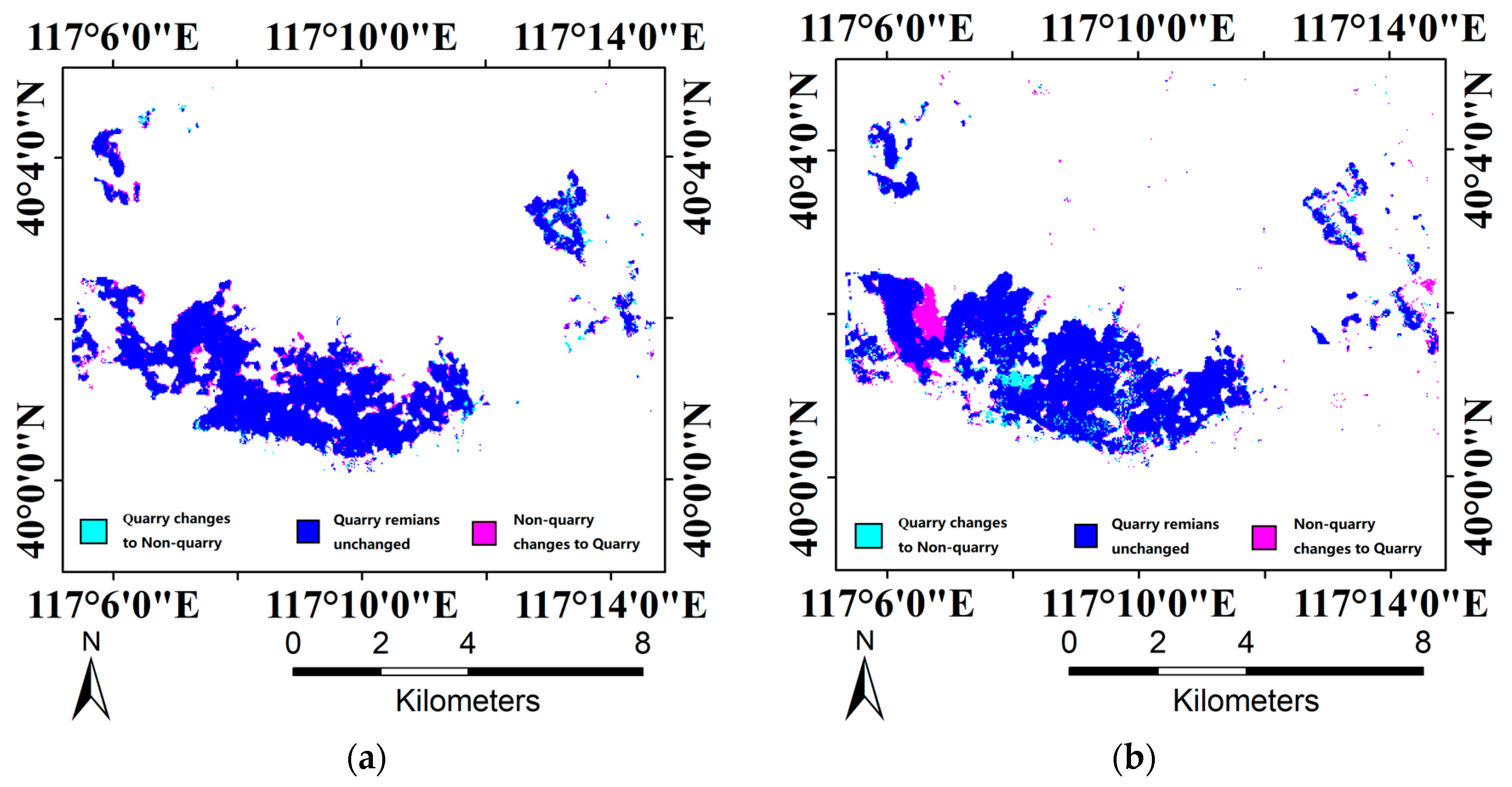
Figure 9.
The study area is split into two regions according to the boundary between Hebei and Tianjin.
Figure 9.
The study area is split into two regions according to the boundary between Hebei and Tianjin.
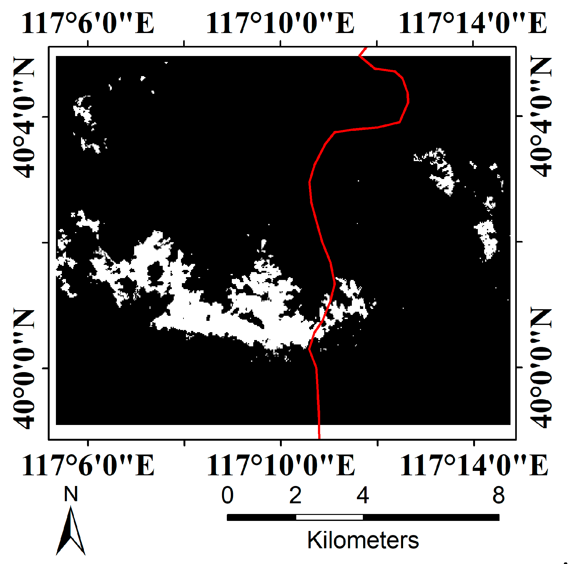
Figure 10.
(a) Quarry area in two regions from 1984 to 2017; (b) Quarry area depicted with two y-axes for the two regions.
Figure 10.
(a) Quarry area in two regions from 1984 to 2017; (b) Quarry area depicted with two y-axes for the two regions.

Figure 11.
(a) Line charts of gross regional products (GRP) in Langfang and the quarry area in Langfang; (b) The scatter diagram of the regression variables before 2009; (c) The scatter diagram of the regression variables after 2009.
Figure 11.
(a) Line charts of gross regional products (GRP) in Langfang and the quarry area in Langfang; (b) The scatter diagram of the regression variables before 2009; (c) The scatter diagram of the regression variables after 2009.

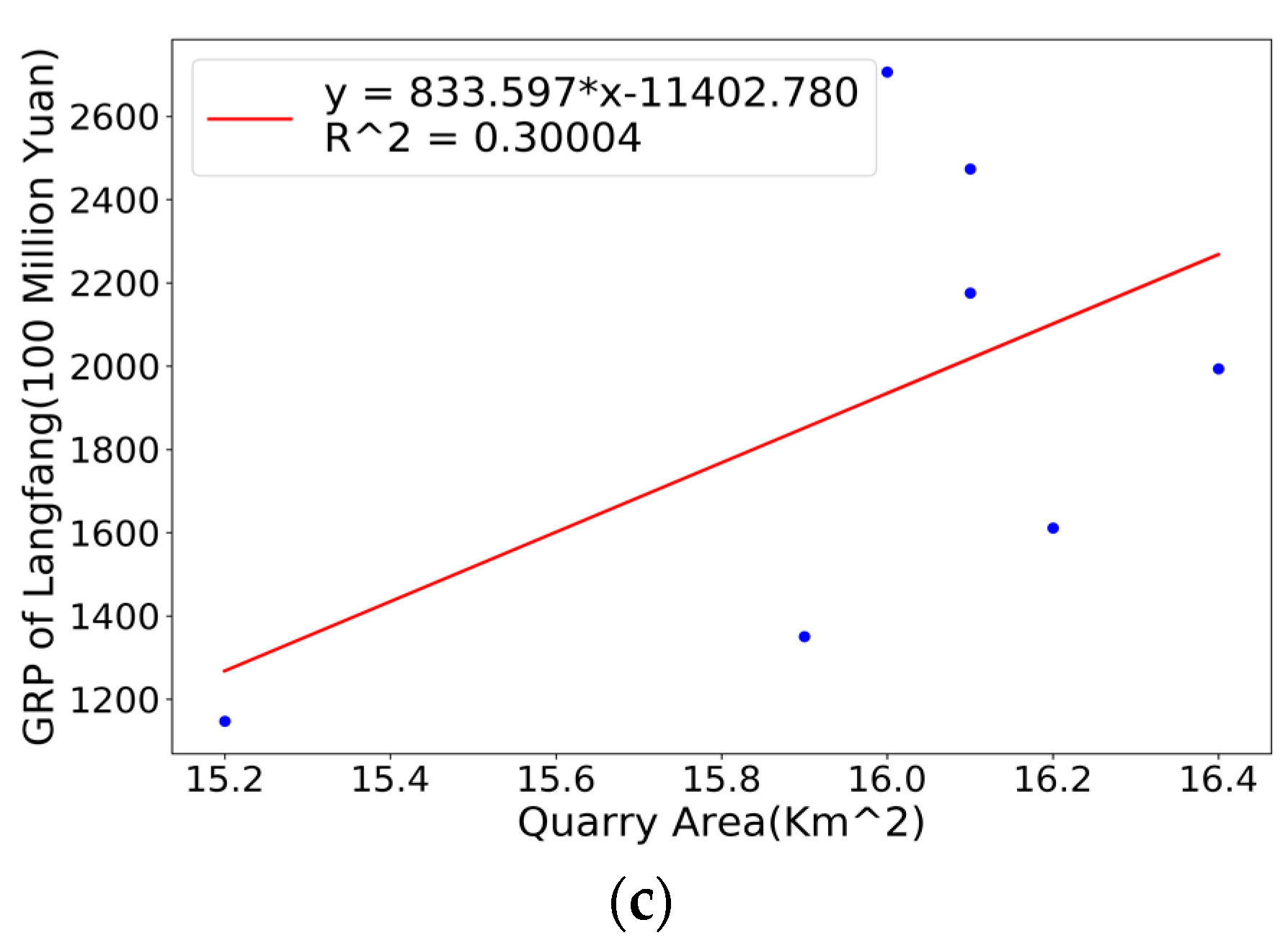
Table 1.
Classification scheme with the number of training samples (number of sample pixels and sample areas in six selected years).
Table 1.
Classification scheme with the number of training samples (number of sample pixels and sample areas in six selected years).
| Year | Class Name | |
|---|---|---|
| Quarry | Non-Quarry (Building, Forest, Farm, Bare Ground) | |
| 1984 | 431 (12) | 21,226 (46) |
| 1992 | 1429 (33) | 19,934 (47) |
| 2002 | 1517 (18) | 17,445 (43) |
| 2010 | 3341 (36) | 17,312 (42) |
| 2013 | 2791 (30) | 16,341 (43) |
| 2016 | 3828 (18) | 18,975 (31) |
Table 2.
Accuracy of the classification results on the ground truth data.
| Year | M-OOB | Kappa | AUC | Year | OOB | Kappa | AUC |
|---|---|---|---|---|---|---|---|
| 1984 | 0.97339 | 0.94199 | 0.99608 | 2001 | 0.97936 | 0.94864 | 0.99724 |
| 1985 | 0.97353 | 0.93944 | 0.99366 | 2002 | 0.97177 | 0.92991 | 0.99689 |
| 1986 | 0.96850 | 0.93227 | 0.99343 | 2003 | 0.93379 | 0.81045 | 0.98081 |
| 1987 | 0.96300 | 0.91500 | 0.99635 | 2004 | 0.95965 | 0.90914 | 0.99326 |
| 1988 | 0.95909 | 0.91005 | 0.99283 | 2005 | 0.97118 | 0.92891 | 0.99508 |
| 1989 | 0.96172 | 0.90129 | 0.99500 | 2006 | 0.97269 | 0.94694 | 0.99616 |
| 1990 | 0.97850 | 0.95124 | 0.99854 | 2007 | 0.96985 | 0.92488 | 0.99293 |
| 1991 | 0.96458 | 0.91188 | 0.99433 | 2008 | 0.96660 | 0.93317 | 0.99408 |
| 1992 | 0.96921 | 0.92225 | 0.99530 | 2009 | 0.97748 | 0.95445 | 0.99669 |
| 1993 | 0.97177 | 0.91871 | 0.99290 | 2010 | 0.97391 | 0.93918 | 0.99476 |
| 1994 | 0.97711 | 0.94931 | 0.99450 | 2011 | 0.97780 | 0.95656 | 0.99722 |
| 1995 | 0.97324 | 0.94332 | 0.99479 | 2013 | 0.94541 | 0.89418 | 0.98797 |
| 1996 | 0.97278 | 0.93496 | 0.99144 | 2014 | 0.95515 | 0.90864 | 0.99157 |
| 1997 | 0.96842 | 0.92273 | 0.99193 | 2015 | 0.94397 | 0.88609 | 0.98819 |
| 1998 | 0.96799 | 0.93110 | 0.98967 | 2016 | 0.96577 | 0.93542 | 0.99557 |
| 1999 | 0.96782 | 0.92415 | 0.99157 | 2017 | 0.95537 | 0.91516 | 0.99353 |
| 2000 | 0.98299 | 0.95761 | 0.99817 |
© 2018 by the authors. Licensee MDPI, Basel, Switzerland. This article is an open access article distributed under the terms and conditions of the Creative Commons Attribution (CC BY) license (http://creativecommons.org/licenses/by/4.0/).
Share and Cite
MDPI and ACS Style
Zhao, H.; Ma, Y.; Chen, F.; Liu, J.; Jiang, L.; Yao, W.; Yang, J. Monitoring Quarry Area with Landsat Long Time-Series for Socioeconomic Study. Remote Sens. 2018, 10, 517. https://doi.org/10.3390/rs10040517
AMA Style
Zhao H, Ma Y, Chen F, Liu J, Jiang L, Yao W, Yang J. Monitoring Quarry Area with Landsat Long Time-Series for Socioeconomic Study. Remote Sensing. 2018; 10(4):517. https://doi.org/10.3390/rs10040517
Chicago/Turabian StyleZhao, Haoteng, Yong Ma, Fu Chen, Jianbo Liu, Liyuan Jiang, Wutao Yao, and Jin Yang. 2018. "Monitoring Quarry Area with Landsat Long Time-Series for Socioeconomic Study" Remote Sensing 10, no. 4: 517. https://doi.org/10.3390/rs10040517
Note that from the first issue of 2016, this journal uses article numbers instead of page numbers. See further details here.