Article

Impacts of Insufficient Observations on the Monitoring of Short- and Long-Term Suspended Solids Variations in Highly Dynamic Waters, and Implications for an Optimal Observation Strategy

1
School of Remote Sensing and Information Engineering, Wuhan University, Wuhan 430079, China
2
State Key Laboratory of Information Engineering in Surveying, Mapping and Remote Sensing, Wuhan University, Wuhan 430079, China
3
Department of Civil and Environmental Engineering, The Hong Kong Polytechnic University, Kowloon, Hong Kong, China
4
State Key Laboratory of Tropical Oceanography, South China Sea Institute of Oceanology, Chinese Academy of Sciences, Guangzhou 510301, China
*
Author to whom correspondence should be addressed.
Remote Sens. 2018, 10(2), 345; https://doi.org/10.3390/rs10020345
Submission received: 7 December 2017 / Revised: 10 February 2018 / Accepted: 16 February 2018 / Published: 23 February 2018

Abstract

:
Coastal water regions represent some of the most fragile ecosystems, exposed to both climate change and human activities. While remote sensing provides unprecedented amounts of data for water quality monitoring on regional to global scales, the performance of satellite observations is frequently impeded by revisiting intervals and unfavorable conditions, such as cloud coverage and sun glint. Therefore, it is crucial to evaluate the impacts of varied sampling strategies (time and frequency) and insufficient observations on the monitoring of short-term and long-term tendencies of water quality parameters, such as suspended solids (SS), in highly dynamic coastal waters. Taking advantage of the first high-frequency in situ SS dataset (at 30 min sampling intervals from 2007 to 2008), collected in Deep Bay, China, this paper presents a quantitative analysis of the influences of sampling strategies on the monitoring of SS, in terms of sampling frequency and time of day. Dramatic variations of SS were observed, with standard deviation coefficients of 48.9% and 54.1%, at two fixed stations; in addition, significant uncertainties were revealed, with the average absolute percent difference of approximately 13%, related to sampling frequency and time, using nonlinear optimization and random simulation methods. For a sampling frequency of less than two observations per day, the relative error of SS was higher than 50%, and stabilized at approximately 10%, when at least four or five samplings were conducted per day. The optimal recommended sampling times for SS were at around 9:00, 12:00, 14:00, and 16:00 in Deep Bay. The “pseudo” MODIS SS dataset was obtained from high-frequency in situ SS measurements at 10:30 and 14:00, masked by the temporal gap distribution of MODIS coverage to avoid uncertainties propagated from atmospheric correction and SS models. Noteworthy uncertainties of daily observations from the Terra/Aqua MODIS were found, with mean relative errors of 19.2% and 17.8%, respectively, whereas at the monthly level, the mean relative error of Terra/Aqua MODIS observations was approximately 10.7% (standard deviation of 8.4%). Sensitivity analysis between MODIS coverage and SS relative errors indicated that temporal coverage (the percentage of valid MODIS observations for a month) of more than 70% is required to obtain high-precision SS measurements at a 5% error level. Furthermore, approximately 20% of relative errors were found with the coverage of 30%, which was the average coverage of satellite observations over global coastal waters. These results highlight the need for high-frequency measurements of geostationary satellites like GOCI and multi-source ocean color sensors to capture the dynamic process of coastal waters in both the short and long term.

Graphical Abstract

1. Introduction

Coastal waters and estuarine systems represent the interface between the land and ocean, and play vital roles in supporting biodiversity and ecosystem functions [1], including global carbon and nutrient cycling and primary production [2]. However, with increasing pressure from both human activities and climate change, coastal ecosystems are under great risk of ecological function degradation and biodiversity loss [3,4,5]. Coastal waters are among the most imperiled ecosystems on Earth [6].Therefore, it is urgent that environmental health is monitored in coastal waters.
The measurement and monitoring of the water constituents in estuarine systems, such as variations of phytoplankton, solids, colored dissolved organic matter, and benthic ecosystems, require continuous measurements over an appropriate period of time. Traditional methods of monitoring water quality are based on in-situ data collection, or sampling with subsequent sample analysis on land or on a ship [7,8], both of which are high-precision but costly and time- and labor-intensive [9]. Moreover, traditional field samples are often too limited in spatial and temporal coverage to build a robust model, or to derive statistically meaningful results [10,11].
Remote sensing data are increasingly used as a rich source of spatial information, providing more detailed coverage than other methods. The superiority of remote sensing for water resource monitoring includes wider spatial coverage, stable long-term acquisition, and low cost compared to conventional methods [12,13]. Therefore, many efforts have been made towards the monitoring of water quality at the local to global scale via remote sensing technology, and considerable progress has been made in studying coastal and inland waters using remote sensing [14,15,16,17]. Conventional ocean color sensors include the proof-of-concept Coastal Zone Color Scanner (CZCS, 1978–1986) and modern radiometers, such as the Sea-viewing Wide Field-of-View Sensor (SeaWiFS, 1997–2010), the Moderate Resolution Imaging Spectroradiometer (Terra/Aqua MODIS, 1999–present), and the Medium Resolution Imaging Spectrometer (Envisat MERIS, 2002–2012), The Ocean and Land Colour Instrument (Sentinel-3A OLCI, 2016–present). Moreover, several new sensors have been launched during the past decade, or are planned to be launched in the next few years, such as the Korean Geostationary Ocean Colour Imager (GOCI, 2010–present), the U.S. Visible Infrared Imager Radiometer Suite (VIIRS, 2011–present), sensors onboard the Chinese HY-series satellites, and The European Space Agency, ESA’s Sentinel-series satellites. Theoretically, these satellite sensors provide comprehensive information about water properties at varied spatial and temporal scales [18,19].
Unfortunately, both the in situ and remote sensing methods for monitoring highly dynamic waters are insufficient in temporal resolution as well as spatial scale, especially for regions with large diurnal or semi-diurnal variations [20,21]. The efficiency and precision of these methods are determined by their sampling strategy (time and interval) because, in most cases, only limited measurements (i.e., once a day or month for in situ monitoring, or twice a day for remote sensing such as Terra/Aqua MODIS) are available, especially for satellite observations, because of cloud contamination, poor weather conditions, and sun glint [22,23]. Adjacency effects should be also considered in near-land areas [24]. Figure 1 shows the temporal coverage of Terra/Aqua MODIS over a typical estuary, Deep Bay, China, with about 23% coverage per month on average. However, the time scale of the coastal water and inland process is about 0.01 h to 10 days, indicating that there is a considerable temporal gap between valid MODIS observations and water quality variations.
Highly dynamic suspended solids (SS) require high-frequency monitoring (observations taken from about every 30 min to 1 h [25]) and an inappropriate sampling strategy would lead to large biases, and thus unscientific decisions during policy-making. Previous research has indicated that an inappropriate sampling strategy could cause a statistical error of more than 50% for water quality monitoring [26,27], and the impacts of missing data were observed in the indicators of annual mean chlorophyll concentration, with a global mean root mean-square error (RMSE) of 8%, whilst higher uncertainty in the peak chlorophyll values was determined as global mean RMSE of 33% [24]. Therefore, it is necessary to quantify the impacts of insufficient SS observations, and to determine the appropriate sampling time and frequency. Moreover, the ongoing satellite ocean color missions call for thorough consideration of the trade-offs between requirements of water resource monitoring and instrument design, including the time and frequency for water quality observation. Although there were some time series stations to monitor the physical, biological, and chemical parameters of water quality—for instance, in the southern North Sea [28], Bohai Sea [29], and in the tidal inlet between the East Frisian islands of Langeoog and Spiekeroog, southern North Sea [30]—high frequency measurements are still rare.
This study aimed to resolve the effects of sampling frequency and sampling time on the monitoring of SS in estuaries, and to assess the uncertainty of the prevailing satellite sensors, Terra/Aqua MODIS, and thus provide a baseline sampling strategy. To achieve this, a two-year, high-frequency, in situ observational SS dataset was first collected in Deep Bay, China, and then the short-term dynamics and temporal variations in the SS were analyzed, followed by error analysis of insufficient observations and an optimization of the sampling strategy.

2. Material and Methods
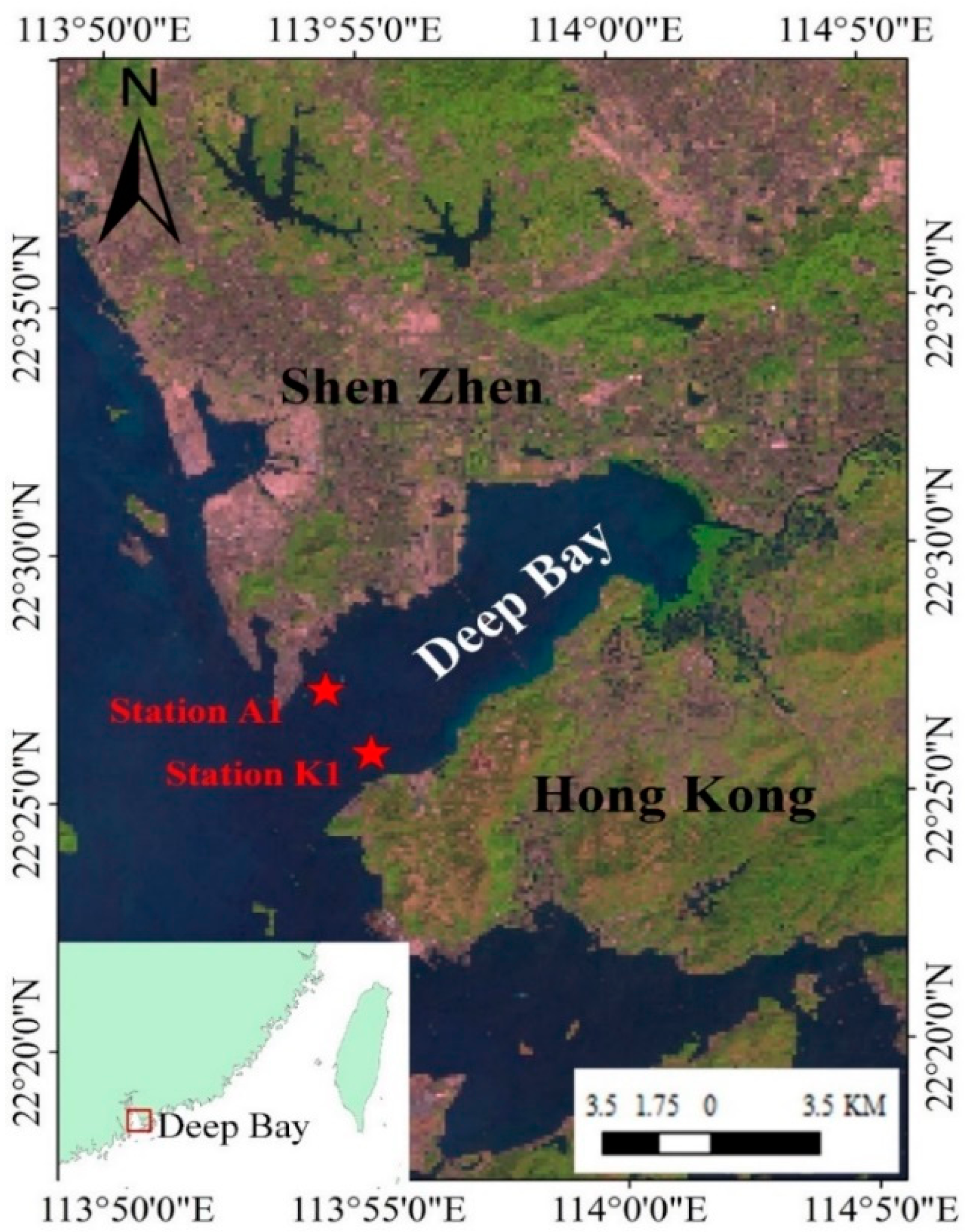
2.1. Study Area

This study was conducted in Deep Bay (22°24′18′′N–22°32′12′′N, 113°53′06′′E–114°02′30′′E), which is located between Shenzhen, a special economic zone of China, to the north, and the New Territories of Hong Kong to the south [31] (Figure 2). Deep Bay is a shallow, semi-enclosed bay on the eastern shore of the Pearl River Estuary, with a width of 4–7.6 km and a length of 13.9 km. The water area of Deep Bay is approximately 80 km2, which is largely enclosed by land and a shallow wetland shore. The margin of fresh water and salt water forms a valuable habitat for a wide variety of life. Influenced by the subtropical oceanic monsoon climate, the rainfall in Deep Bay is concentrated from April to September, and the dry season is from October to March.
With the rapid urbanization of Shenzhen, the northern shoreline of Deep Bay has been reclaimed for building land. In addition, Deep Bay has been subjected to extensive anthropogenic pollutants emitted by villages and livestock farms (as noted by the Environmental Protection Department (EPD) Marine Water Quality in Hong Kong in 2004), and the water quality has been evaluated to be one of the worst around Hong Kong (from the EPD Marine Water Quality in Hong Kong in 2006). This anthropogenic enhancement of nutrients can be expected to result in eutrophication, which is a major threat to the sensitive associated marine ecosystems (wetland reserves) and oyster culturing in the bay [32,33,34]. Since the area around Deep Bay has rapidly urbanized, it is urgent to develop a good understanding of water quality in the bay, as it is located close to human society.

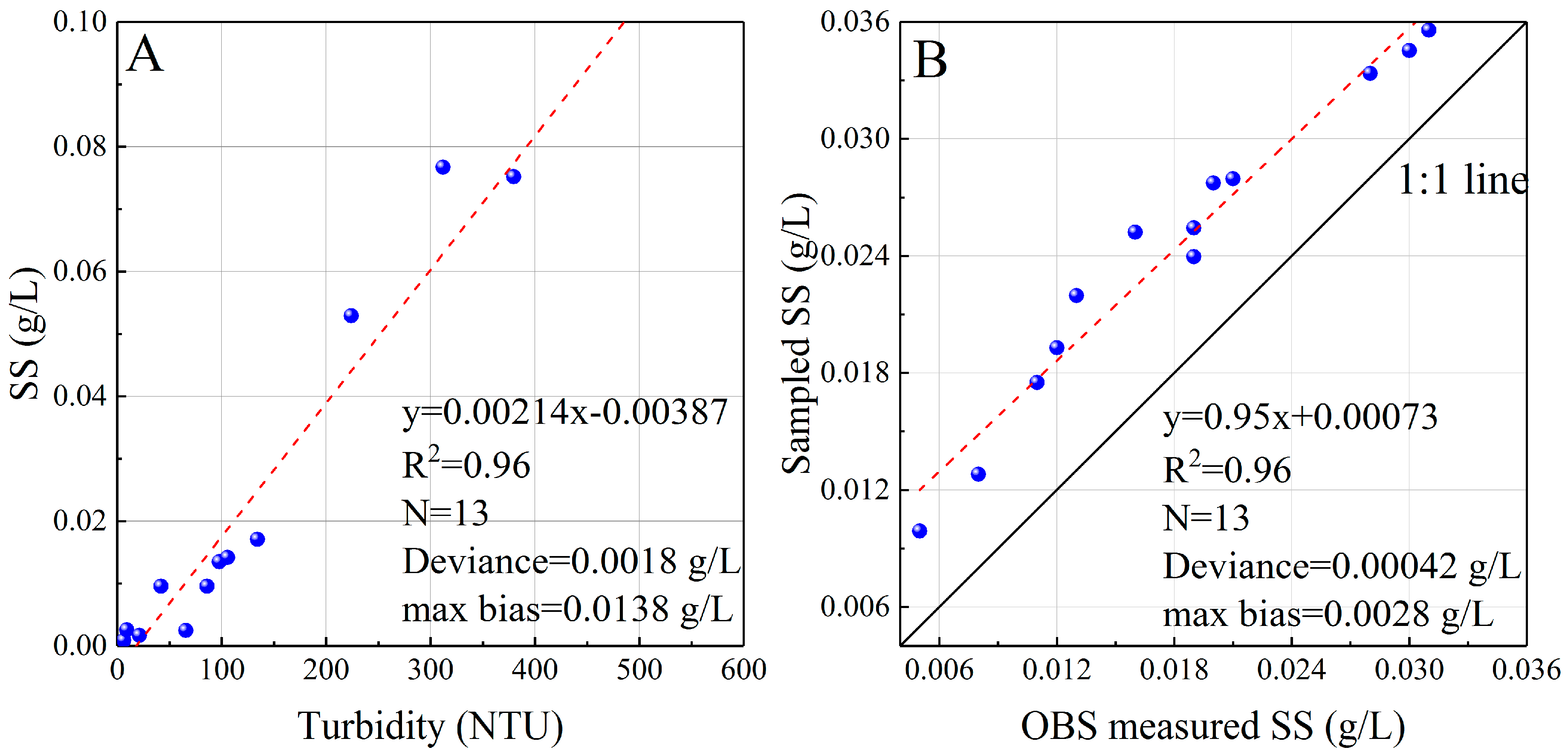
2.2. Fixed Stations and Measurements

The SS measurements were conducted at two fixed stations (A1 to the north and K1 to the south) in Deep Bay (Figure 2). The two stations are located at the intersection of Deep Bay and the Pearl River, with an average local water depth of about 3.0 m, and the sensor at a depth of about 0.8 m below the water surface, to ensure that the sensors would be submerged during the measuring time. The in situ measurements were collected from January 2007 to December 2008 (two years in total), and 48 measurements were obtained at half-hour intervals during the period of 0:00 to 23:30 each day.
A backward light scattering sensor (OBS-3a turbidity sensor, the D&A Instrument Company, https://www.campbellsci.com/obs-3a) was used for SS measurement, as it can provide accurate and reliable estimates of SSC [35].The range of the OBS measurement is 0 to approximately 5 kg/m3 for suspended particulate material, and 0 to approximately 4000 NTU for turbidity. In addition, the accumulation of biomaterial around the submerged sensors is a major problem to overcome, in order to ensure that the measured data, which were cleared during the routine maintenance, are accurate [28].
To ensure that the data were credible, the OBS instrument was maintained every 7 to 10 days, and calibration of the OBS was conducted using simultaneously collected field water samples. The water samples were stored and transported to the laboratory, and filtered through 47 mm glass fiber filters, to obtain the SS concentration using a weighing method [36]. The water sample was filtered with a 470 nm filter (Whatman GF/F filters) and vacuum filtration system. The filter pad was flushed with 0.00005 m3 of distilled water 3 times, in order to flush away the salt. The dry weight of the filter pad was weighed with an electronic analytic scale. The blank filter and sampled filter pad were weighed until the difference between two successive SS concentrations calculated from the scale reading was within 0.01 mg/L [31].
During each calibration, at least 10 matchups (Matchups-1) of turbidity measured by OBS and laboratory-analyzed SS were collected for cross calibration, and another 10 matchups or more (Matchups-2) for validation of the calibration results. The water samples of Matchups-1 were collected before and after the OBS was cleaned, to ensure the relationship between the SS and turbidity would not change as biomaterial around the submerged sensors had accumulated in the short period. The results of regression analysis on the calibration between OBS-measured turbidity and laboratory-analyzed SS on 2 March 2007 is shown in Figure 3A, and the coefficient of the determination (R2) between them was 0.96, with a deviance of 0.018 g/L and max bias of 0.138 g/L. In addition, the regression results between OBS measured SS and laboratory-analyzed SS are shown in Figure 3B, where the R2 was 0.96, with a deviance of 0.0042 g/L and max bias of 0.0028 g/L.
The routine maintenance of the OBS sensors was performed about every 7 to 10 days, during which the sensors were cleaned, the data were transferred, and the battery was recharged. The calibration of the sensor was conducted about every month, and 26 or 25 calibrations were performed in total for stations A1 and K1, respectively, as listed in Table 1. Descriptions of the in situ data collection and sensor calibrations (once a month) were also provided in a previous study ([37,38], in Chinese with English abstract).
The spatial variability of SS at in situ stations is important for satellite based SS modeling and validation, especially when there are significant differences of spatial scale between in situ data and remote sensing data. The spatial variances of stations A1 and K1 use high spatial resolution GF-1 satellite data (16 m spatial resolution), using SS model of our previous study [39]. The mean values (and standard deviation) of SS around A1 and K1 were 0.0476 (0.0016) and 0.0423 (0.0012) g/L, respectively, which were relatively small, and could represent the general case of SS around the study area.

2.3. Remote Sensing Observations

MODIS is a key instrument on board the Terra and Aqua satellites, which were launched by the National Aeronautics and Space Administration (NASA) in 1999 and 2001, respectively (http://modis.gsfc.nasa.gov). With advantages including medium spatial resolution (250 m, 500 m, 1000 m), multi-spectral detectors of 36 spectral bands between 0.405 and 14.385 µm, daily coverage, high radiometric sensitivity, and free-access distribution [40], MODIS data have been frequently employed to retrieve SS data during the past decade. Furthermore, the two MODIS sensors have collected more than 10 years’ worth of data on the Earth’s surface, and this image archive provides a great opportunity to monitor and analyze the long-term spatiotemporal dynamics of parameters of the Earth’s surface, such as SS [41]. Many studies have shown the potential to detect water components and concentrations in complex waters with MODIS data [39,42,43].
Despite the widespread use of MODIS data, the precision of short- and long-term monitoring using MODIS is determined by its sampling strategy (observing time and frequency), because in most cases only limited measurements are available, especially for satellite observations with cloud contamination, poor weather conditions, and sun glint. Table 1 shows the temporal coverage of Terra/Aqua MODIS over Deep Bay, with about 45% and 28% coverage for 2007 and 2008, on average. Most months had coverage of lower than 50%, which means that less than 15 observations are available for these months. However, the time scale of the coastal and inland water process was about 0.01 h to 10 days, indicating a temporal gap between valid observations and water quality variations. Therefore, it is critical to assess the impacts of insufficient observations, and to determine the optimal sampling strategies from high-frequency in situ measurements.
In general, conventional technology for acquiring satellite-based SS requires radiometric calibration, atmospheric correction, SS modeling, and validation to obtain reliable SS estimations. In this paper, MODIS-derived SS were not directly used, due to large uncertainties (around 30%) of SS from propagation errors of atmospheric correction and SS models [44,45,46,47,48], no matter what regional empirical models or semi-analytical models were used, especially at coastal or inland optically-complex waters. Instead, MODIS-measured SS were “simulated” using in-situ OBS-measured SS at 10:30 and 14:00, and the MODIS gap distribution (Table 2) of valid MODIS observations from 2007 to 2008 was used as a mask, which was applied to the two-year high-frequency in situ SS measurements, in order to obtain a “pseudo” or “simulated” MODIS SS dataset. This dataset was free of the uncertainties of satellite-derived SS, to evaluate the impact that MODIS sampling time and frequency may have on the estimation of SS. Specifically, we evaluated the precision and accuracy of SS by computing the relative errors and the bias arising purely from missing data, so no actual satellite data or models were used for this study.

2.4. Analysis Methods

A statistical approach was employed to the continuous time series data from the two field stations. Five statistical parameters—the mean, the maximum, the minimum, the standard deviation (STD), and the standard deviation coefficient (SDC)—were selected to depict the variations of the SS. The STD and SDC were calculated by using the following formulas:
S T D = i = 1 N ( B i μ ) 2 N
S D C = S T D μ · 100 %
where N is the total number of SS observations at each station, B i is the ith observation, and μ is the mean value of the N observations.
Nonlinear optimization was employed to determine the optimal observation time for SS sampling. Nonlinear optimization problems appear in many applications, including parameter identification and optimal control, and nonlinear optimization has emerged as a key technology in modern scientific applications. Challenges include optimization problems, with partial differential equations as constraints—for example, optimization problems for flows, transport problems, diffusion processes, wave propagation, or mechanical structures. An efficient solution to such problems requires highly-developed optimization methods, which use modern adaptive multilevel techniques of scientific computing. “Lingo”, an optimization modeling software and coding languages for building and solving linear, nonlinear, and integer models (https://www.lindo.com/), is used for nonlinear optimization. Lingo provides a completely integrated package for expressing optimization models, and allows a user to quickly build a model, solve it, and assess the correctness or appropriateness of the model based on the solution, which is faster, easier, and more efficient [49].
Nonlinear optimization was adopted in this study to solve the problem of how to achieve the minimal observation error with the minimum number of observations and corresponding time. Hence, the objective function of the nonlinear optimization is to calculate the minimal observation error as follows:
Y = i M ( | j N B i j N X ¯ i | / X ¯ i ) / M
where Y is the objective function of relative errors from different sampling strategies (sampling number and corresponding time), M is the duration of the observations (days, months or years), N is the number of observations, X i ¯ is the average value of all the observations, Bij is the jth observation of the ith day in the selected month or year. N was defined from 1 to 48, since we obtained 48 measurements of SS each day, and all combinations of the N observations among the 48 observations were randomly selected and tested. The value of N corresponding to the minimum Y among the 48 Y values were then determined. We defined the average value of the 48 measurements as the truly observed result of the day (here, we supposed the measurements have no gross error and thus there is no need to eliminate the gross error).
To assess the biases of insufficient observation of satellites versus in situ data, some parameters in [50] were adopted, including the root mean square deviation (RMSD), the determination coefficient (R2), the average of percent differences (ψ), and the average of absolute (unsigned) percent differences (|ψ|) of match-ups between simulated remote sensing SS and in situ SS. The RMSD and R2 determine whether the match-ups are stable and relevant, and the quantity ψ and |ψ| determine the bias and the scattering of data points, respectively [50].
The value of ψ and |ψ| are calculated through
ψ = 1 N i = 1 N ψ i
| ψ | = 1 N i = 1 N | ψ i |
where i is the match-up index and ψ i is
ψ i = 100 · S S ( i ) S I ( i ) S I ( i )
with the superscripts S and I indicating the simulated and the in situ data, respectively.

3. Results

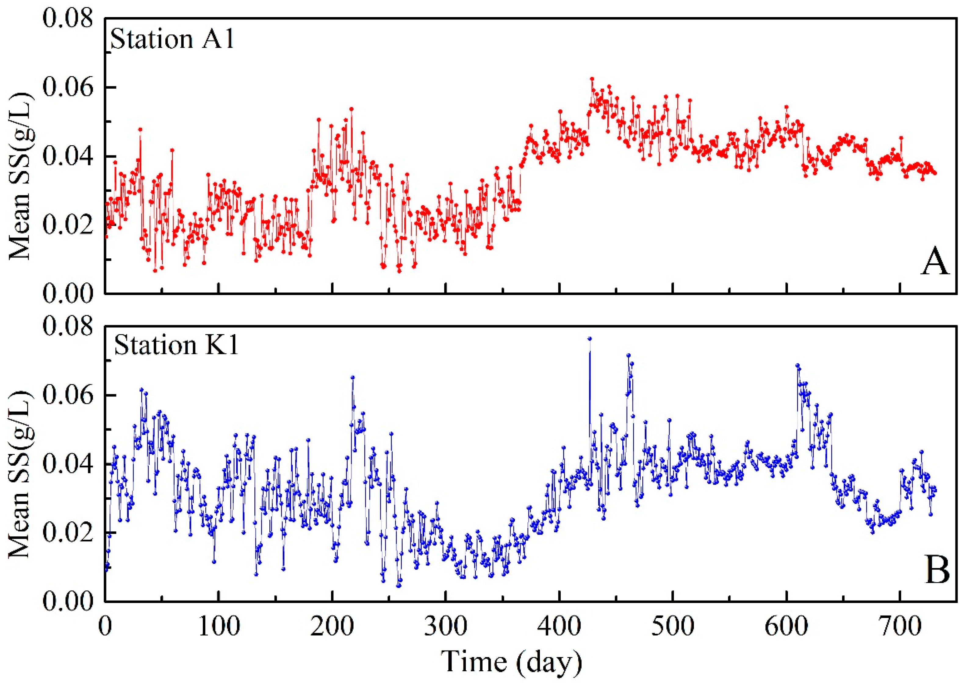
3.1. Variations of SS in Deep Bay

During the in situ measurement period from January 2007 to December 2008, 35,088 samples were collected in total for stations A1 and K1 (Figure 4). These continuous and high-frequency measurements of the SS provided the first basic data for examination of temporal variation and the development of an appropriate sampling strategy. Highly dynamic SS variations were observed in Deep Bay. The ratios of the maximum to the minimum SS in a day varied from 1.188 to 66, indicating that considerable variation of SS in Deep Bay can be expected during a month, and even within a day.
Table 3 presents statistical parameters for SS in 2007 and 2008 at the two stations. The mean values were 0.0341 and 0.0324 g/L at stations A1 and K1, respectively, and the SDCs at the two stations were 48.94% and 54.07%, respectively, indicating that the variation of SS was similar at the two stations. However, the SDC values at stations A1 and K1 in 2007 were 67.59% and 62.00%, respectively, while those in 2008 were 22.94% and 44.83%, respectively, indicating that the SS varied more substantially in 2007 than in 2008.
Since substantial variation in SS concentration was shown in Deep Bay, it is necessary to determine the optimal time and number of observations when monitoring the sediment change in Deep Bay, to improve monitoring results for these waters.

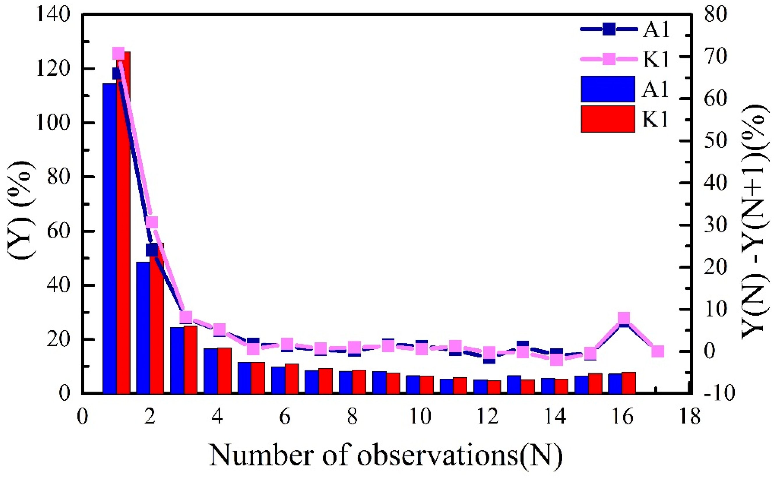
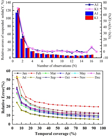
3.2. Errors Associated with Frequency of Observation for the SS Estimations

The relative errors (Y) of different number of observations (N) of SS were obtained from nonlinear optimization. After selecting N observations among 48 observations, we might have C 48 N choices. Next, the optimal combination of N was found based on the minimum error. Figure 5 shows the Y value (%) for a varied number of observations N, together with the first-order error differences between N and N + 1. Both stations A1 and K1 showed similar results, indicating the method is valid and could be expanded to other regions.
The decreasing trend of Y with the increasing number of observations N is revealed in Figure 5. For N = 1, Y could exceed 100%, and N = 2 would reduce Y to about 50%. Therefore, it is important to increase the number of observations, to constrain a low level of relative error. When N was increased to four or five times per day, Y stabilized at about 10%, and subsequent increases to N would not improve the accuracy of the SS measurements. Note that the first-order error differences between N and N + 1 (line in Figure 5) remained stable when N exceeded five.
Although increasing the number of measurements could improve the accuracy of observed results, it is important to point out that it also means increasing consumption of manpower, material resources, and financial expense. It is therefore important to identify a suitable number of observations. Based on Figure 5, it is reasonable to conclude that when we have four to five observations in a day, the Y value of SS measurements could be constrained to 15%. Moreover, little improvement in Y could be made by increasing the number of observations after N is larger than five observations per day, since the first-order difference is nearly zero.

3.3. Errors Associated with Observation Times for the SS Estimations

Section 3.2 demonstrated the impacts of the number of observations on the accuracy of SS estimation. Furthermore, it is crucial to determine the optimal sampling time, which would provide a practical guide for SS monitoring. For instance, there are C 48 5 combinations for a total of five observations, and identification of the optimal time combination is required for SS monitoring. Table 4 presents relative errors (Y) of the SS estimation associated with N and the corresponding time. Since the first-order error difference was stabilized at nearly zero when N was larger than five observations per day, it is not necessary to discuss cases involving more observations.
Results showed that the best time combinations to measure the SS at the Deep Bay were nearly identical at both stations, with the time difference within half an hour, except when there was only one observation in a day. The consistency between the two stations also provided a cross validation of the methods and results, since the two stations were both located at Deep Bay, and were thus affected by similar forcing factors. For a single observation, the optimal sampling time was found to be between about 13:00 and 14:00, but the relative errors were higher than 110% even at the optimal sampling time. However, it should be noted that the sampling frequency of most existing measurement methods is not more than once per day (N = 1). When N was increased to 2, the relative errors dropped considerably to the level of about 50%, and then the sampling times were determined to be at 11:00 and around 15:30. Similarly sampling time combinations for N of 3, 4 or 5 were obtained, and after N reached 5, the relative errors remained at about the 10% level.
Furthermore, the time interval between each observation was also important for the optimal sampling strategy. As shown in Table 4, if N = 2, then the time interval between each observation would be about 4 to 5 h. For N = 3, the time interval would be 3 h. When N = 4 or 5, the time interval between observations would be less than 2 h, and the relative error would decrease little regardless of whether the observations increase or not. Therefore, the threshold in this case was set to 2 h. When the time interval is less than 2 h, the accuracy for SS monitoring will not be substantially improved.

4. Discussion

MODIS is a widely used remote sensing sensor for water quality monitoring, because of its medium spatial resolution, daily coverage, high sensitivity, and open-access distribution [40]. Considering its widespread application in both environmental protection and scientific research fields [39,42,51,52,53], it is urgent to assess the uncertainties of MODIS data in SS monitoring, because of the existing temporal gap between MODIS temporal coverage and variations of SS (Figure 1 and Table 1). Therefore, the assessment of uncertainties in SS monitoring with insufficient remote sensing observations not only provides detailed information on the reliability of the most commonly used data, but also offers guidance for future sampling strategies, for both in situ measurements and remote sensing observations. In this context, uncertainties caused by insufficient remote sensing observations are assessed here for two cases: the temporal coverage of the first case was determined by the designed indicator of MODIS, which is an ideal case or the top bound of the MODIS observations; and the second case was set as the actual conditions of MODIS observations, which is affected by cloud contamination, poor weather conditions, and sun glint [20,22,23].

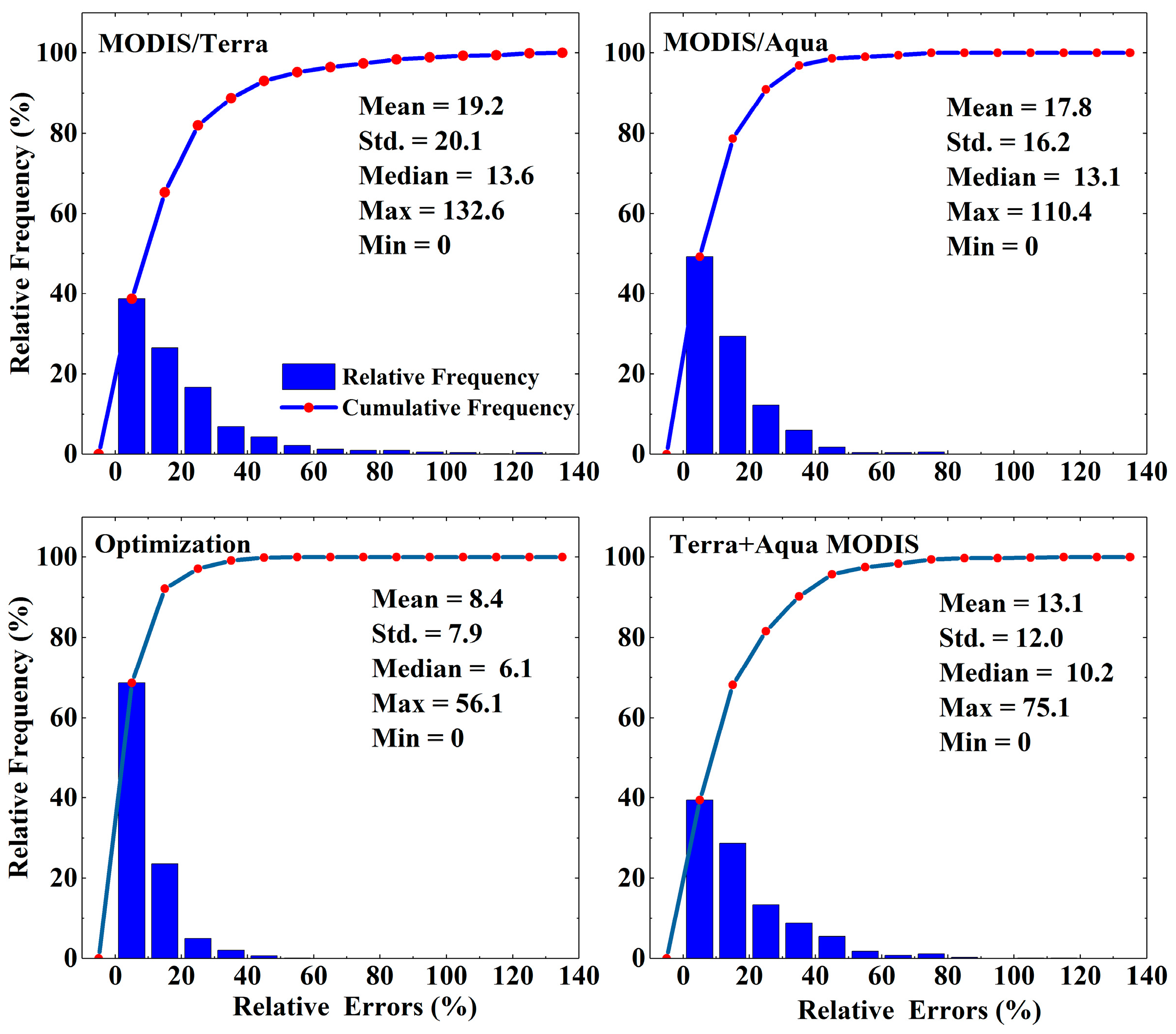
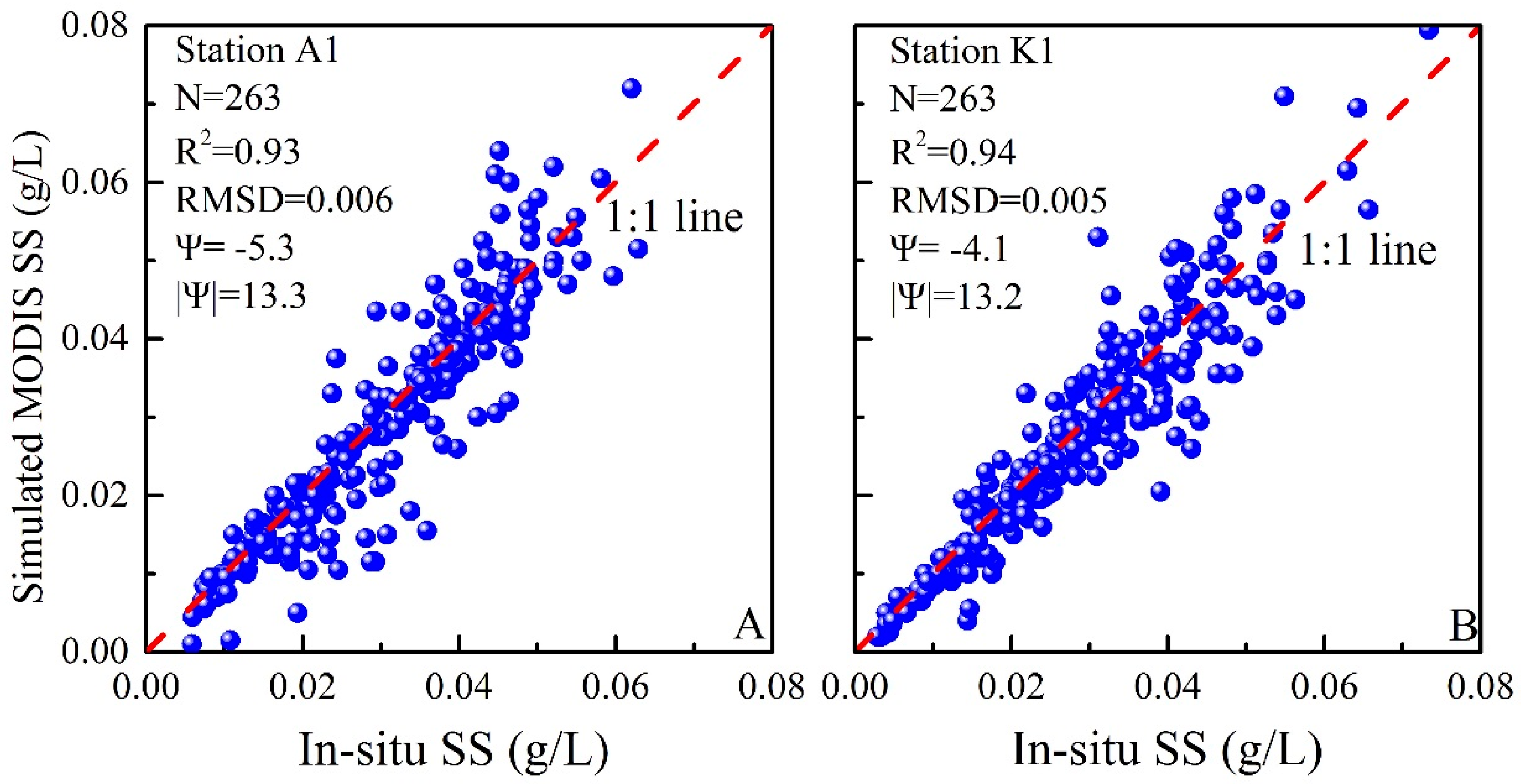
4.1. Estimating Errors of Satellite Remote Sensing

4.1.1. Daily Scale Observations

The MODIS sensor onboard the Terra and Aqua satellites takes pictures of the Earth twice a day, at 11:00 for MODIS/Terra and 13:00 for MODIS/Aqua local time in Deep Bay. The in situ data from January 2007 to December 2008 were used as reference, and the data measured at 11:00 and 13:00 were picked out as simulated MODIS/Terra and MODIS/Aqua observations.
The parameters and scatters plots of simulated SS from MODIS (Terra and Aqua) versus in situ SS and the optimized SS versus in-situ SS are shown in Figure 6. The relative error of MODIS/Terra, MODIS/Aqua, combination of MODIS/Terra and MODIS/Aqua, and the optimization result (the SS measurements obtained by the best combinations of observation frequency and time using the nonlinear optimization method described in Section 2.4) were calculated and compared. The relative errors of MODIS/Terra, MODIS/Aqua, combination of MODIS/Terra and MODIS/Aqua, and the results of the optimization are shown in Figure 7. Overall, the negative bias indicated by ψ decreased from 4–5% to 1–2%, and the mean absolute percent differences (|ψ|) decreased from ~13% to ~7%.
Note that only results at station A1 are presented for brevity, since results at station K1 and A1 were almost identical. The single observation of MODIS/Terra or MODIS/Aqua produced mean (±STD) relative errors of 19.2% (±20.1%) and 17.8% (±16.2%), respectively. The relative error could be reduced to 13.1% (±12.0%) by a combination of the observations from MODIS/Terra and MODIS/Aqua. The optimized observation strategy showed the smallest relative error of 8.4% (±7.9%). Moreover, the daily relative errors were smaller in 2008 than in 2007 at both stations. This may be because of the variations of SS, as depicted by the SDC. The SDC at stations A1 and K1 in 2007 were 67.59% and 62.00%, whereas in 2008 they were 22.94% and 44.83%, respectively. Therefore, the SS varied more substantially in 2007 than that in 2008.
Figure 8 presents the frequency statistics of relative errors of varied observation strategies of SS at station A1. The frequency histogram of relative errors of the optimization results was concentrated near 10%, while the distribution of error histograms was more dispersed when using single observations from MODIS/Terra or MODIS/Aqua. However, when observations from MODIS/Terra and MODIS/Aqua were combined, uncertainties caused by insufficient sampling were largely reduced. Compared with the single MODIS/Terra or MODIS/Aqua observations, the performance of the SS measurements was improved by 32.3% and 19.1% on average by the combination of the two sensors, respectively.

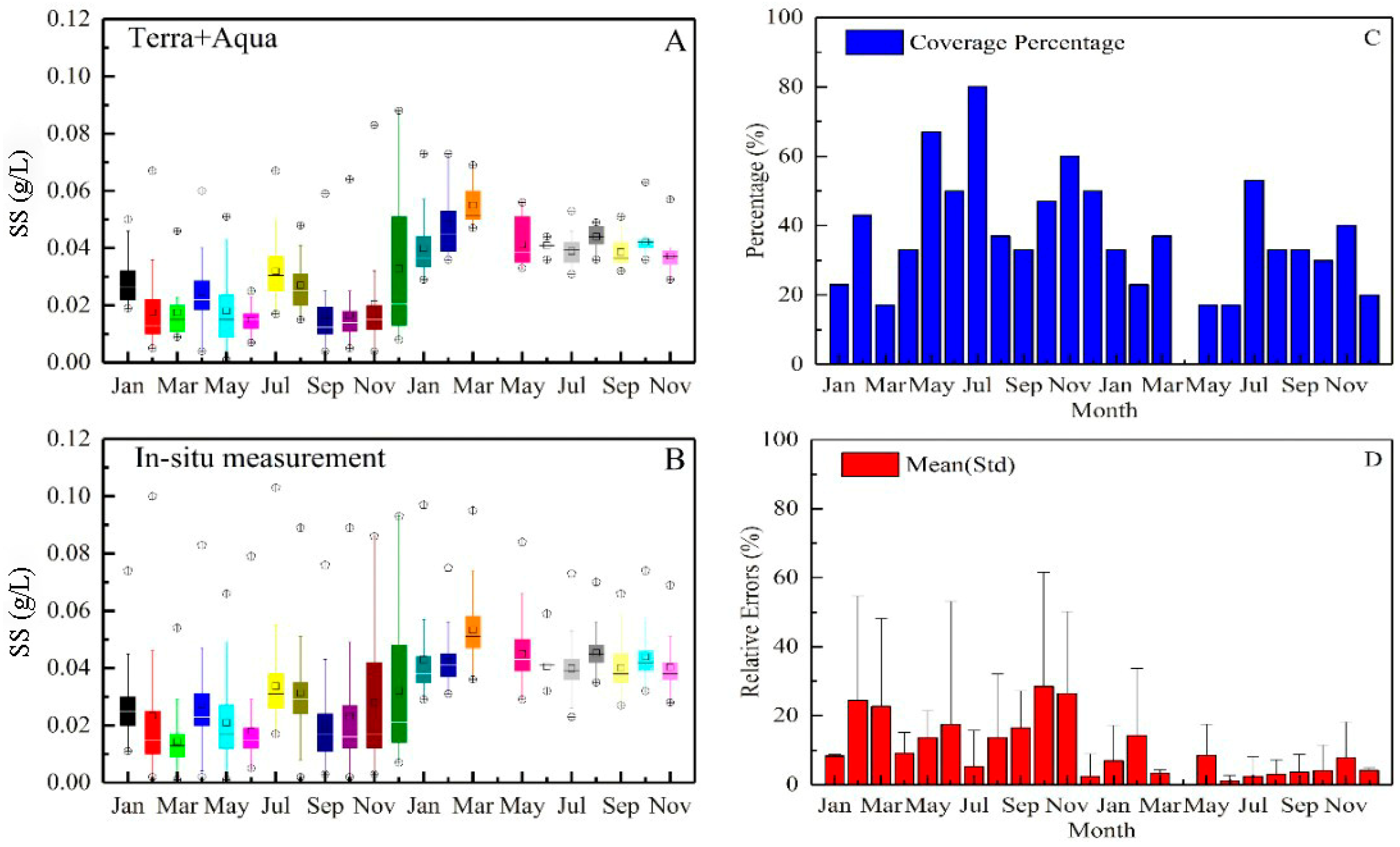
4.1.2. Monthly Scale Observations

In situ, two-year SS time series data were used as a reference to assess the uncertainties caused by insufficient satellite observations. To reduce uncertainties from remote-sensing-derived SS products, satellite-measured SS were “simulated” using in situ reference data. The in situ, two-year time series were masked by the valid overpass timetable of the satellite (Table 2), to simulate the distribution of missing data in the two-year MODIS remote sensing measurements, thus generating an in situ time series with MODIS-like gaps; then, uncertainties caused by MODIS-like missing data were calculated with the in situ reference time series.
Uncertainties caused by insufficient observations of satellite remote sensing were analyzed at the monthly scale, as shown in Figure 9. The average monthly coverage of remote sensing observations was 45% and 28% for 2007 and 2008, respectively (Table 2 and Figure 9C), and except for April 2008, there were generally more than five valid observations in a month. Although the monthly statistics and trends of SS obtained from combined MODIS/Terra and MODIS/Aqua and in situ measurements showed similar variations (Figure 9A,C), relative errors between the two datasets were high (Figure 9D). The average relative error of satellite observations was 10.7% (STD of 8.4%), while an opposite trend was found for the coverage. The peak relative error values generally appeared when the coverage was relatively low, and vice versa. The magnitudes of the correlations were different between 2007 and 2008, as shown in Figure 9D, with higher relative errors and higher coverage in 2007 than in 2008. The annual variations of the relative errors were also influenced by the degree of SS variations, which were affected by tide, wind speed, and wind direction. As discussed in Section 3.1, the variations of SS were greater in 2007 than in 2008, which could explain why the relative errors were larger in 2007 than in 2008.
The impacts of insufficient satellite observations on the statistical results of SS monitoring were further analyzed for the maximum and minimum values (Table 5). The relative errors of these statistical indicators were significant, though mean values and the trend of SS were comparable between MODIS observations and in situ data. The average relative errors of maximum and minimum SS from valid MODIS observations were 25.9% and 35.2%, respectively, which were higher than the relative error of the statistical average of SS (10.7%). This implies that when aiming to monitor the maximum and minimum SS, insufficient satellite observations are more prone to be unable to capture these indicators. Compared with the in situ measurements, a limited number of valid satellite observations significantly underestimated the maximum SS and overestimated the minimum SS. For instance, the maximum SS was underestimated by 59.7% in June, and the minimum SS was overestimated by 66.3% in July.

4.1.3. Annual Scale Observations

Although evident uncertainty from insufficient MODIS observations was found in SS monitoring at daily or monthly scales, such uncertainty was reduced at the annual scale. Table 6 represents the annual mean SS of MODIS\Aqua, MODIS\Terra, the in situ data, and the relative errors of the satellite sensors measurements. The largest relative error was found to be 18.05%, which was much smaller than errors observed at daily at monthly scale. One possible reason for such a phenomenon may lie in the fact that on an annual scale, inner-annual variations of SS were prone to be omitted, and thus the influence of insufficient observation was less significant.
While the accuracy of average SS monitoring is strongly related to the coverage of satellite observation (higher coverage leads to lower relative error), the insufficient remote sensing data showed little relation to the maximum and minimum SS. Therefore, it is critical to assess the impacts of limited remote sensing data on the validity of SS monitoring. Moreover, the analysis in this section also suggests that uncertainties of the most widely used Terra/Aqua MODIS data need be considered for coastal water monitoring.

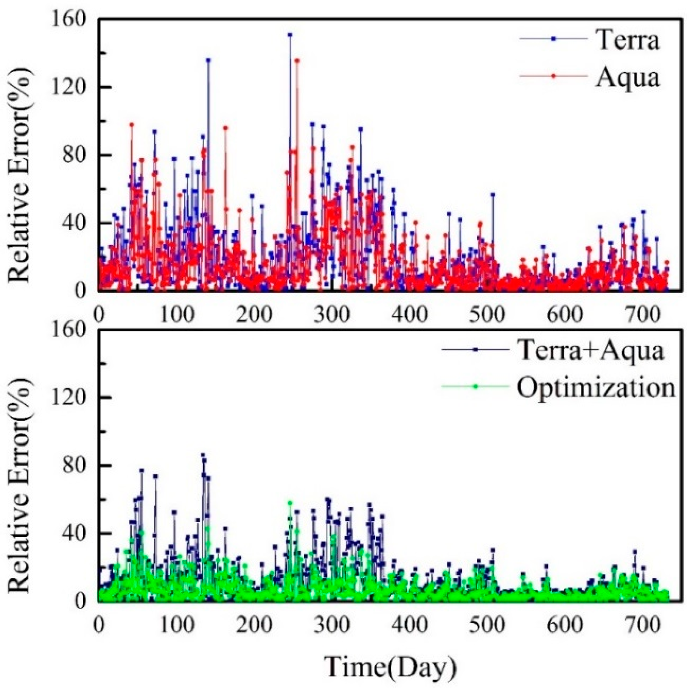
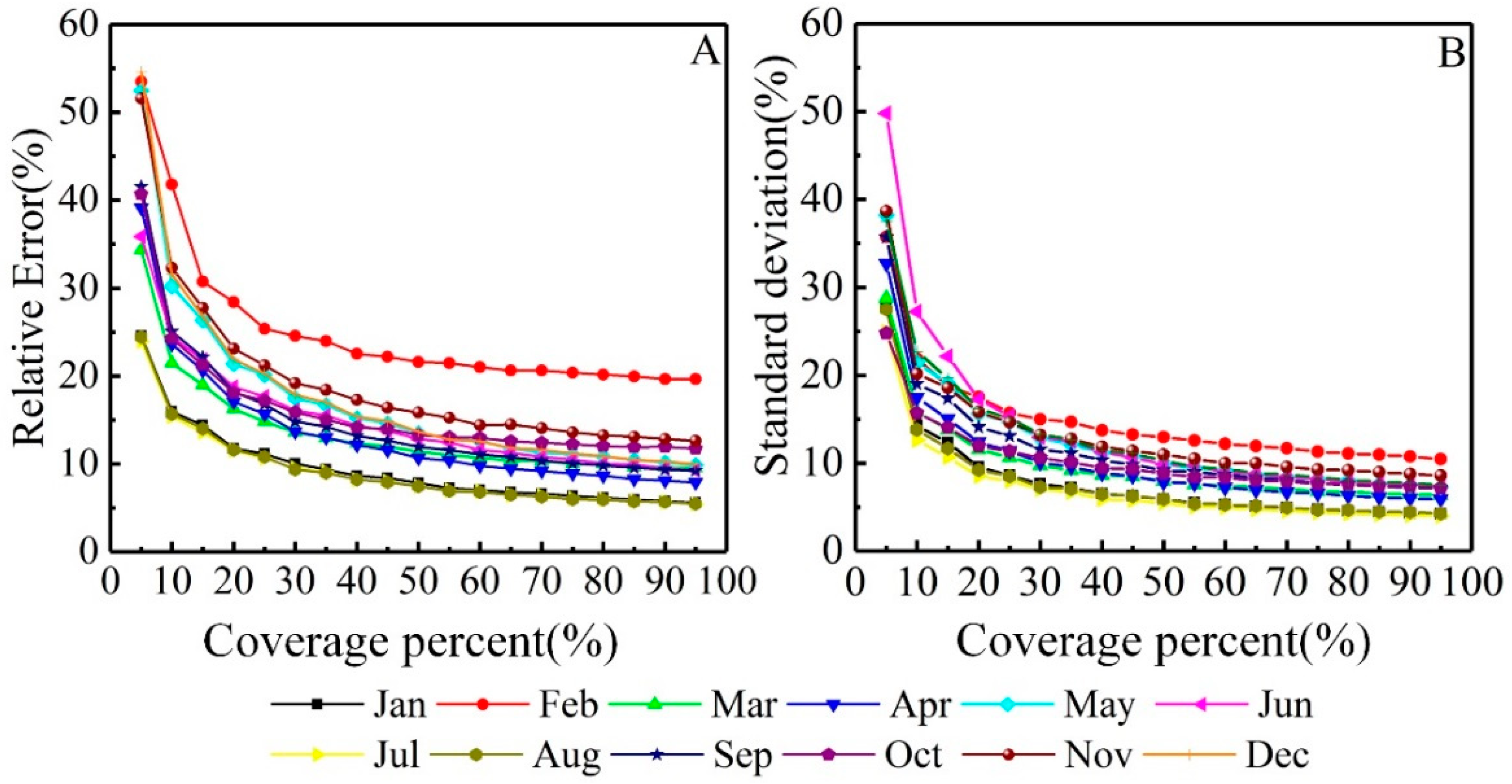
4.2. Sensitivity of SS Monitoring with Satellite Coverage

Sensitivity analyses were conducted to determine how the precision of SS monitoring is affected by satellite coverage, and thus provide reference information for historical data quality assessment and future SS observation strategy. A random simulation method was applied to calculate the monthly mean relative errors of SS measurements with different levels of satellite coverage, from 5% to 95%, in intervals of 5%. For each coverage each month at the A1 and K1 stations, the combination of valid observations was chosen randomly, and the relative errors were calculated 10,000 times to produce stable results.
Figure 10 presents variations of the monthly mean relative errors and standard deviations under different satellite coverage levels. A remarkably decreasing tendency in relative error and uncertainties of the SS measurements was found with increasing coverage. For coverage lower than 10%, the monthly relative errors and standard deviations reached approximately 50%, and decreased to about 20% when the coverage increased to 30%, and then stabilized at approximately 5% when the coverage increased to 70%. Although there were some fluctuations among different months, the trends of all results were similar, which permits flexible applications of the analysis to wider spatial and temporal ranges.
It is important to clarify that insufficient satellite observations are common, despite extensive applications of remote sensing in coastal and inland water quality monitoring. For instance, the sun-synchronous polar orbiting satellite sensor provided approximately 110 cloud-free observation days per year in the Southern North Sea [54], at about 30.1% cloud coverage. A total of 7–12 valid observations from ENVISAT-MERIS were obtained for Lake Vänern in Sweden in August 2003 [55]. Furthermore, pioneering research showed that the mean daily percentage of valid observations of surface ocean chlorophyll a concentrations from MODIS is generally <20% for most oceans [56]. In addition, the impacts of clouds and sun glint prevent any single satellite from observing more than about 15% of the ocean surface in a single day [57].
The mean cloud coverage of global oceans was calculated from valid Terra/MODIS observations from between 2002 and 2016. In general, cloud coverage is extremely high around the global ocean, especially for latitudes >30°N and >30°S, which have larger than 60% cloud coverage on average; areas between 0°–30°N and 0°–30°S typically have lower cloud coverage. The Chinese regions of ocean and coast are dominated by cloud coverage at the level of approximately 65% to 70%. According to the results of this study and previous research, great uncertainties from insufficient satellite observations would be induced in water quality archives and environmental data records that have been widely applied for social and scientific communities. Sampling biases in monthly and annual mean chlorophyll estimates from MODIS were calculated to reach nearly 8%, under the irregular temporal coverage of ocean color sensors [26]. Similarly, the impacts of missing data were observed in the indicators of annual mean chlorophyll concentration with a global mean RMSE of 8%, whilst higher uncertainty in the peak chlorophyll values was determined as a global mean RMSE of 33%, and a bias of approximately 20% [23]. These figures and our results both highlight the need to quantify uncertainties in frequently-used satellite products [58] and the need to optimize our observation strategy.

5. Implications and Conclusions

Motivated by urgent needs for coastal or inland water quality monitoring and rapid expansions of available satellite data, a great effort has been made by numerous research studies [17,54,59]. Despite the great progress achieved in remote sensing of the water environment, as well as instruments and protocols of field observations, reliability evaluations of the past and present remote sensing data, which are critical under unfavorable conditions like cloud coverage and sun glint, are rare [22,23]. Caution should be taken when limited satellite observations are used in water quality estimations, in consideration of the considerable uncertainties from insufficient observations.
Taking advantage of the first high-frequency in situ SS dataset collected in the coastal waters of Deep Bay, China, the effects of sampling frequency and sampling time on the monitoring of highly dynamic SS were resolved in this study. Results demonstrated the major influences of sampling strategy on SS observations, including the number and frequency of sampling. Relative errors related to the number of observations were stabilized at approximately 10% when at least four or five samples were taken per day, and the optimal sampling times were recommended using nonlinear optimization. Noteworthy uncertainties of daily observations from Terra/Aqua MODIS were found with mean relative errors of 19.2% and 17.8%, respectively. The monthly mean relative error of Terra/Aqua MODIS observations was approximately 10.7% (STD of 8.4%). The results of this paper are consistent with previous research [23,26], but also highlight the need for high-frequency measurements to capture the dynamic processes of coastal or inland waters in both the short and long term.
The high-frequency datasets used in this paper will undoubtedly provide researchers with abundant information that would otherwise be very difficult or expensive to obtain at larger spatial scales. As shown in the presented case study, the imbalance between highly dynamic processes and insufficient satellite observations of water quality is common. Therefore, optimization of the sampling strategy to fully exploit available earth observation resources is recommended. Owing to the rapid expansion of satellite sensors and open data policy, the combination of multiple satellite sensors could considerably improve the performance of remote sensing data. For instance, the relative error could be reduced to 13.1% by the combination of observations from Terra and Aqua MODIS, whereas the relative error from a single MODIS/Terra or MODIS/Aqua observation was 19.2% and 17.8%, respectively. Furthermore, present geostationary ocean color satellite sensors, COMS-GOCI, and the scheduled GEO-CAPE could provide great opportunities for the monitoring of high-frequency temporal variability in coastal or inland waters, and for a better understanding of inland and coastal waters.

Acknowledgements

This work was supported by the National Natural Science Foundation of China (Nos. 41701379, 41571344, 41331174, 41071261, 40906092, 40971193, 41101415, 41401388, 41206169, and 41406205), Special Fund by Surveying & Mapping and Geoinformation Research in the Public Interest (201512026), the China Postdoctoral Science Foundation, the program of Key Laboratory for National Geographic Census and Monitoring, National Administration of Surveying, Mapping and Geoinformation (No. 2014NGCM), Natural Science Foundation of Jiangxi, China (No. 20161BAB213074), Wuhan University Luojia Talented Young Scholar project, Dragon 4 proposal ID 32442, entitled “New Earth Observations tools for Water resource and quality monitoring in Yangtze wetlands and lakes (EOWAQYWET)”, the Open Research Fund of the Key Laboratory of Space Ocean Remote Sensing and Application, State Oceanic Administration People’s Republic of China (No. 201502003), LIESMARS Special Research Funding, the High Resolution Earth Observation Systems of National Science and Technology Major Projects (41-Y20A31-9003-15/17), LIESMARS Special Research Funding, the “985 Project” of Wuhan University; Special funds of State Key Laboratory for equipment.

Author Contributions

Qu Zhou and Jian Li conceived and designed the experiments; Qu Zhou performed the experiments; Liqiao Tian and Jian Li helped to outline the manuscript structure; and Onyx W. H. Wai and Zhaohua Sun helped Qu Zhou and Wenkai Li to prepare the manuscript.

Conflicts of Interest

The authors declare no conflict of interest.

References

  1. Gleick, P.; White, F. Water in Crisis: A Guide to the World's Fresh Water Resources; Oxford University Press: New York, NY, USA, 1993. [Google Scholar]
  2. Bastviken, D.; Tranvik, L.J.; Downing, J.A.; Crill, P.M.; Enrich-Prast, A. Freshwater methane emissions offset the continental carbon sink. Sciences 2011, 331, 50–55. [Google Scholar] [CrossRef] [PubMed]
  3. Allan, J.D.; McIntyre, P.B.; Smith, S.D.P.; Halpern, B.S.; Boyer, G.L.; Buchsbaum, A.; Burton, G.A.; Campbell, L.M.; Chadderton, W.L.; Ciborowski, J.J.H.; et al. Joint analysis of stressors and ecosystem services to enhance restoration effectiveness. Proc. Natl. Acad. Sci. USA 2013, 110, 372–377. [Google Scholar] [CrossRef] [PubMed]
  4. Heath, M.R. Comment on “a global map of human impact on marine ecosystems”. Sciences 2008, 321, 948–952. [Google Scholar] [CrossRef] [PubMed] [Green Version]
  5. Torbick, N.; Hession, S.; Hagen, S.; Wiangwang, N.; Becker, B.; Qi, J. Mapping inland lake water quality across the lower peninsula of michigan using landsat tm imagery. Int. J. Remote Sens. 2013, 34, 7607–7624. [Google Scholar] [CrossRef]
  6. Dudgeon, D.; Arthington, A.H.; Gessner, M.O.; Kawabata, Z.; Knowler, D.J.; Lévêque, C.; Naiman, R.J.; Prieur-Richard, A.H.; Soto, D.; Stiassny, M.L. Freshwater biodiversity: Importance, threats, status and conservation challenges. Biol. Rev. Camb. Philos. Soc. 2006, 81, 163–182. [Google Scholar] [CrossRef] [PubMed]
  7. O’Shea, M.L.; Brosnan, T.M. Trends in indicators of eutrophication in western long island sound and the hudson-raritan estuary. Estuaries Coasts 2000, 23, 877. [Google Scholar] [CrossRef]
  8. Paerl, H.W.; Valdes, L.M.; Piehler, M.F.; Stow, C.A. Assessing the effects of nutrient management in an estuary experiencing climatic change: The neuse river estuary, north carolina. Environ. Manag. 2006, 37, 422–436. [Google Scholar] [CrossRef] [PubMed]
  9. Glasgow, H.B.; Burkholder, J.A.M.; Reed, R.E.; Lewitus, A.J.; Kleinman, J.E. Real-time remote monitoring of water quality: A review of current applications, and advancements in sensor, telemetry, and computing technologies. J. Exp. Mar. Biol. Ecol. 2004, 300, 409–448. [Google Scholar] [CrossRef]
  10. Zolfaghari, K.; Duguay, C. Estimation of water quality parameters in lake erie from meris using linear mixed effect models. Remote Sens. 2016, 8, 473. [Google Scholar] [CrossRef]
  11. Joshi, I.D.; D’Sa, E.J.; Osburn, C.L.; Bianchi, T.S.; Dong, S.K.; Oviedo-Vargas, D.; Arellano, A.R.; Ward, N.D. Assessing chromophoric dissolved organic matter (cdom) distribution, stocks, and fluxes in apalachicola bay using combined field, viirs ocean color, and model observations. Remote Sens. Environ. 2017, 191, 359–372. [Google Scholar] [CrossRef]
  12. Ritchie, J.C.; Zimba, P.V.; Everitt, J.H. Remote sensing techniques to assess water quality. Photogramm. Eng. Remote Sens. 2003, 69, 695–704. [Google Scholar] [CrossRef]
  13. Wang, Y.; Xia, H.; Fu, J.; Sheng, G. Water quality change in reservoirs of shenzhen, china: Detection using landsat/tm data. Sci. Total Environ. 2004, 328, 195. [Google Scholar] [CrossRef] [PubMed]
  14. Mouw, C.B.; Greb, S.; Aurin, D.; DiGiacomo, P.M.; Lee, Z.; Twardowski, M.; Binding, C.; Hu, C.; Ma, R.; Moore, T.; et al. Aquatic color radiometry remote sensing of coastal and inland waters: Challenges and recommendations for future satellite missions. Remote Sens. Environ. 2015, 160, 15–30. [Google Scholar] [CrossRef]
  15. Feng, L.; Hu, C.; Chen, X.; Cai, X.; Tian, L.; Gan, W. Assessment of inundation changes of poyang lake using modis observations between 2000 and 2010. Remote Sens. Environ. 2012, 121, 80–92. [Google Scholar] [CrossRef]
  16. Matthews, M.W.; Bernard, S.; Robertson, L. An algorithm for detecting trophic status (chlorophyll-a), cyanobacterial-dominance, surface scums and floating vegetation in inland and coastal waters. Remote Sens. Environ. 2012, 124, 637–652. [Google Scholar] [CrossRef]
  17. Mcclain, C.R.; Meister, G. Mission Requirements for Future Ocean-Colour Sensors; International Ocean-Colour Coordinating Group (IOCCG) Report Series, No. 13; IOCCG: Dartmouth, NS, Canada, 2012. [Google Scholar]
  18. Hu, C.; Feng, L.; Lee, Z.; Davis, C.O.; Mannino, A.; Mcclain, C.R.; Franz, B.A. Dynamic range and sensitivity requirements of satellite ocean color sensors: Learning from the past. Appl. Opt. 2012, 51, 6045. [Google Scholar] [CrossRef] [PubMed]
  19. Maritorena, S.; D’Andon, O.H.F.; Mangin, A.; Siegel, D.A. Merged satellite ocean color data products using a bio-optical model: Characteristics, benefits and issues. Remote Sens. Environ. 2010, 114, 1791–1804. [Google Scholar] [CrossRef]
  20. Choi, J.-K.; Park, Y.J.; Ahn, J.H.; Lim, H.-S.; Eom, J.; Ryu, J.-H. Goci, the world’s first geostationary ocean color observation satellite, for the monitoring of temporal variability in coastal water turbidity. J. Geophys. Res. Oceans 2012, 117, 4–9. [Google Scholar] [CrossRef]
  21. Ody, A.; Doxaran, D.; Vanhellemont, Q.; Nechad, B.; Novoa, S.; Many, G.; Bourrin, F.; Verney, R.; Pairaud, I.; Gentili, B. Potential of high spatial and temporal ocean color satellite data to study the dynamics of suspended particles in a micro-tidal river plume. Remote Sens. 2016, 8, 245. [Google Scholar] [CrossRef] [Green Version]
  22. Kaufman, Y.J.; Remer, L.A.; Tanre, D.; Li, R.R.; Kleidman, R.; Mattoo, S.; Levy, R.C.; Eck, T.F.; Holben, B.N.; Ichoku, C. A critical examination of the residual cloud contamination and diurnal sampling effects on modis estimates of aerosol over ocean. IEEE Trans. Geosci. Remote Sens. 2005, 43, 2886–2897. [Google Scholar] [CrossRef]
  23. Racault, M.F.; Sathyendranath, S.; Platt, T. Impact of missing data on the estimation of ecological indicators from satellite ocean-colour time-series. Remote Sens. Environ. 2014, 152, 15–28. [Google Scholar] [CrossRef]
  24. Goyens, C.; Jamet, C.; Schroeder, T. Evaluation of four atmospheric correction algorithms for modis-aqua images over contrasted coastal waters. Remote Sens. Environ. 2013, 131, 63–75. [Google Scholar] [CrossRef]
  25. Antoine, D. Ocean-Colour Observations from a Geostationary Orbit; International Ocean-Colour Coordinating Group (IOCCG) Report Series, No. 12; IOCCG: Dartmouth, NS, Canada, 2012. [Google Scholar]
  26. Gregg, W.W.; Casey, N.W. Sampling biases in modis and seawifs ocean chlorophyll data. Remote Sens. Environ. 2007, 111, 25–35. [Google Scholar] [CrossRef]
  27. Chen, Z.; Hu, C.; Muller-Karger, F.E.; Luther, M.E. Short-term variability of suspended sediment and phytoplankton in tampa bay, florida: Observations from a coastal oceanographic tower and ocean color satellites. Estuar. Coast. Shelf Sci. 2010, 89, 62–72. [Google Scholar] [CrossRef]
  28. Garaba, S.P.; Badewien, T.H.; Braun, A.; Schulz, A.C.; Zielinski, O. Using ocean colour remote sensing products to estimate turbidity at the wadden sea time series station spiekeroog. J. Eur. Opt. Soc. 2014, 9, 1–6. [Google Scholar] [CrossRef]
  29. Zhou, Z.; Bian, C.; Wang, C.; Jiang, W.; Bi, R. Quantitative assessment on multiple timescale features and dynamics of sea surface suspended sediment concentration using remote sensing data. J. Geophys. Res. Oceans 2017, 122, 8739–8752. [Google Scholar] [CrossRef]
  30. Reuter, R.; Badewien, T.H.; Bartholomä, A.; Braun, A.; Lübben, A.; Rullkötter, J. A hydrographic time series station in the wadden sea (southern north sea). Ocean Dyn. 2009, 59, 195–211. [Google Scholar] [CrossRef]
  31. Tian, L.; Wai, O.; Chen, X.; Liu, Y.; Feng, L.; Li, J.; Huang, J. Assessment of total suspended sediment distribution under varying tidal conditions in deep bay: Initial results from hj-1a/1b satellite ccd images. Remote Sens. 2014, 6, 9911–9929. [Google Scholar] [CrossRef]
  32. Hun, J.; Wei, L.; Qian, A. Three-Dimensional Modeling of Hydrodynamic and Flushing in Deep Bay. In Proceedings of the International Conference on Estuaries & Coasts, Hangzhou, China, 9–11 November 2003; pp. 9–11. [Google Scholar]
  33. Smith, V.H.; Joye, S.B.; Howarth, R.W. Eutrophication of freshwater and marine ecosystems. Limnol. Oceanogr. 2006, 51, 351–355. [Google Scholar] [CrossRef]
  34. Jie, X.; Yin, K.D.; Lee, J.H.W.; Liu, H.B.; Ho, A.Y.T.; Yuan, X.C.; Harrison, P.J.; Zingone, A.; Phlips, E.J.; Harrison, P.J. Long-term and seasonal changes in nutrients, phytoplankton biomass, and dissolved oxygen in deep bay, hong kong. Estuaries Coasts 2010, 33, 399–416. [Google Scholar]
  35. Downing, J. Twenty-five years with obs sensors: The good, the bad, and the ugly. Cont. Shelf Res. 2006, 26, 2299–2318. [Google Scholar] [CrossRef]
  36. Le, C.F.; Li, Y.M.; Yong, Z.; Sun, D.Y.; Yin, B. Validation of a quasi-analytical algorithm for highly turbid eutrophic water of meiliang bay in taihu lake, china. IEEE Trans. Geosci. Remote Sens. 2009, 47, 2492–2500. [Google Scholar]
  37. Jian, Q.; Liang, B.; Wang, T.; Chen, J.; Zhang, H. Research on online-monitoring method and practice of obs-3a. J. Changjiang Eng. Vocat. Coll. 2008, 25, 28–31. [Google Scholar]
  38. Chang, L.; Peng, Y.; Huang, H. Application of new instruments and equipments in shenzhen river hydrological measurement. J. Changjiang Eng. Vocat. Coll. 2012, 29, 23–24. [Google Scholar]
  39. Tian, L.; Wai, O.W.H.; Chen, X.; Li, W.; Li, J.; Li, W.; Zhang, H. Retrieval of total suspended matter concentration from gaofen-1 wide field imager wfi multispectral imagery with the assistance of terra modis in turbid water—Case in deep bay. Int. J. Remote Sens. 2016, 37, 3400–3413. [Google Scholar] [CrossRef]
  40. Miller, R.L.; McKee, B.A. Using modis terra 250 m imagery to map concentrations of total suspended matter in coastal waters. Remote Sens. Environ. 2004, 93, 259–266. [Google Scholar] [CrossRef]
  41. Wu, G.; Cui, L.; He, J.; Duan, H.; Fei, T.; Liu, Y. Comparison of modis-based models for retrieving suspended particulate matter concentrations in poyang lake, china. Int. J. Appl. Earth Obs. Geoinf. 2013, 24, 63–72. [Google Scholar] [CrossRef]
  42. Doxaran, D.; Lamquin, N.; Park, Y.J.; Mazeran, C.; Ryu, J.H.; Wang, M.; Poteau, A. Retrieval of the seawater reflectance for suspended solids monitoring in the east china sea using modis, meris and goci satellite data. Remote Sens. Environ. 2014, 146, 36–48. [Google Scholar] [CrossRef]
  43. Wang, W.; Jiang, W. Study on the seasonal variation of the suspended sediment distribution and transportation in the east china seas based on seawifs data. J. Ocean Univ. China 2008, 7, 385–392. [Google Scholar] [CrossRef]
  44. Nechad, B.; Ruddick, K.G.; Park, Y. Calibration and validation of a generic multisensor algorithm for mapping of total suspended matter in turbid waters. Remote Sens. Environ. 2010, 114, 854–866. [Google Scholar] [CrossRef]
  45. Sun, D.; Li, Y.; Le, C.; Shi, K.; Huang, C.; Gong, S.; Yin, B. A semi-analytical approach for detecting suspended particulate composition in complex turbid inland waters (china). Remote Sens. Environ. 2013, 134, 92–99. [Google Scholar] [CrossRef]
  46. Wang, J.J.; Lu, X.X. Estimation of suspended sediment concentrations using terra modis: An example from the lower yangtze river, china. Sci. Total Environ. 2010, 408, 1131–1138. [Google Scholar] [CrossRef] [PubMed]
  47. Tarrant, P.E.; Amacher, J.A.; Neuer, S. Assessing the potential of medium-resolution imaging spectrometer (meris) and moderate-resolution imaging spectroradiometer (modis) data for monitoring total suspended matter in small and intermediate sized lakes and reservoirs. Water Resour. Res. 2010, 46, 2973–2976. [Google Scholar] [CrossRef]
  48. IOCCG. Remote Sensing of Ocean Colour in Coastal, and Other Optically-Complex, Waters; IOCCG: Dartmouth, NS, Canada, 2000. [Google Scholar]
  49. Schrage, L. Optimization Modeling with Lingo; Lindo System: Chicago, IL, USA, 2006. [Google Scholar]
  50. Zibordi, G.; Mélin, F.; Berthon, J.F.; Canuti, E. Assessment of meris ocean color data products for european seas. Ocean Sci. 2013, 9, 521–533. [Google Scholar] [CrossRef]
  51. Zhao, W.J.; Wang, G.Q. Assessment of seawifs, modis, and meris ocean colour products in the south china sea. Int. J. Remote Sens. 2014, 35, 4252–4274. [Google Scholar] [CrossRef]
  52. Feng, L.; Hu, C.; Chen, X.; Song, Q. Influence of the three gorges dam on total suspended matters in the yangtze estuary and its adjacent coastal waters: Observations from modis. Remote Sens. Environ. 2014, 140, 779–788. [Google Scholar] [CrossRef]
  53. Petus, C.; Marieu, V.; Novoa, S.; Chust, G.; Bruneau, N.; Froidefond, J.M. Monitoring spatio-temporal variability of the adour river turbid plume (bay of biscay, france) with modis 250-m imagery. Cont. Shelf Res. 2014, 74, 35–49. [Google Scholar] [CrossRef] [Green Version]
  54. Ruddick, K.; Neukermans, G.; Vanhellemont, Q.; Jolivet, D. Challenges and opportunities for geostationary ocean colour remote sensing of regional seas: A review of recent results. Remote Sens. Environ. 2014, 146, 63–76. [Google Scholar] [CrossRef]
  55. Philipson, P.; Kratzer, S.; Ben Mustapha, S.; Strömbeck, N.; Stelzer, K. Satellite-based water quality monitoring in lake vänern, sweden. Int. J. Remote Sens. 2016, 37, 3938–3960. [Google Scholar] [CrossRef]
  56. Feng, L.; Hu, C. Comparison of valid ocean observations between modis terra and aqua over the global oceans. IEEE Trans. Geosci. Remote Sens. 2016, 54, 1575–1585. [Google Scholar] [CrossRef]
  57. Gregg, W.W.; Esaias, W.E.; Feldman, G.C.; Frouin, R.; Hooker, S.B.; Mcclain, C.R.; Woodward, R.H. Coverage opportunities for global ocean color in a multimission era. IEEE Trans. Geosci. Remote Sens. 1998, 36, 1620–1627. [Google Scholar] [CrossRef]
  58. Barnes, B.B.; Hu, C. Cross-sensor continuity of satellite-derived water clarity in the gulf of mexico: Insights into temporal aliasing and implications for long-term water clarity assessment. IEEE Trans. Geosci. Remote Sens. 2014, 53, 1761–1772. [Google Scholar] [CrossRef]
  59. Palmer, S.C.J.; Kutser, T.; Hunter, P.D. Remote sensing of inland waters: Challenges, progress and future directions. Remote Sens. Environ. 2015, 157, 1–8. [Google Scholar] [CrossRef]
Figure 1. Temporal coverage of Terra/ Aqua MODIS over Deep Bay (A), and spatial-temporal variation scales of coastal/inland waters (B) (reproduced from Mouw, 2015, [14]).
Remotesensing 10 00345 g001
Figure 2. Location of Deep Bay, and the in situ measurements of suspended solids (SS) at stations A1 and K1.
Remotesensing 10 00345 g002
Figure 3. Regression results between turbidity measured by the OBS sensors and the suspended solids (SS) obtained from water samples (A), and between SS measured by the OBS sensors and the in situ SS obtained in water samples (B).
Remotesensing 10 00345 g003
Figure 4. Daily mean suspended solids (SS) from 2007 to 2008 at station A1 (A) and K1 (B).
Remotesensing 10 00345 g004
Figure 5. Relative errors (Y, bars) corresponding to the number of observations (N), and the first order error differences (Y(N) – Y(N + 1), lines) between N and N + 1.
Remotesensing 10 00345 g005
Figure 6. Scatter plots and biases of SS from MODIS (Terra + Aqua) versus in situ SS match-ups at station A1 (A) and K1 (B).
Remotesensing 10 00345 g006
Figure 7. Relative errors of MODIS/Terra, MODIS/Aqua, the combination of MODIS/Aqua and MODIS/Terra, and the optimization results at station A1.
Remotesensing 10 00345 g007
Figure 8. Frequency statistics of relative errors of MODIS/Terra, MODIS/Aqua, the combination of MODIS/Aqua and MODIS/Terra, and the optimization results at station A1.
Remotesensing 10 00345 g008
Figure 9. Monthly suspended solids (SS) of valid MODIS observations (A), in situ measurements (B), monthly coverage of MODIS observations (C), and relative errors between MODIS and in situ measurements (D).
Remotesensing 10 00345 g009
Figure 10. Monthly relative errors (A) and standard deviations (B) under different coverage of satellite observations.
Remotesensing 10 00345 g010
Table 1. Calibration models of OBS sensor during the field measurements. (Date format: yyyy/mm/dd).
StationDateRegression Model
(y: SS; x: Turbidity)
StationDateRegression Model
(y: SS; x: Turbidity)
A12007/1/5y = 0.00097x − 0.00138 K12007/1/5y = 0.00100x − 0.00027
2007/2/3y = 0.00136x − 0.01892 2007/3/1y = 0.00119x − 0.00056
2007/3/2y = 0.00214x − 0.00387 2007/3/18y = 0.00118x + 0.00306
2007/3/16y = 0.00090x − 0.00489 2007/4/4y = 0.00115x + 0.00147
2007/4/5y = 0.00098x − 0.00264 2007/5/5y = 0.00126x − 0.00517
2007/4/22y = 0.00097x − 0.00330 2007/5/16y = 0.00125x − 0.00154
2007/5/15y = 0.00095x − 0.00979 2007/6/5y = 0.00170x − 0.00667
2007/6/1y = 0.00100x − 0.00717 2007/7/1y = 0.00125x − 0.00212
2007/7/3y = 0.00116x + 0.00645 2007/7/23y = 0.00125x − 0.00009
2007/7/19y = 0.00096x + 0.00705 2007/8/16y = 0.00154x + 0.00716
2007/7/23y = 0.00116x + 0.00645 2007/8/30y = 0.00114x + 0.00625
2007/8/18y = 0.00127x − 0.00527 2007/9/5y = 0.00150x − 0.00463
2007/9/2y = 0.00098x − 0.00304 2007/10/20y = 0.00111x − 0.00522
2007/10/26y = 0.00141x − 0.00883 2007/11/6y = 0.00112x − 0.00821
2007/11/6y = 0.00135x − 0.007312007/12/23y = 0.00114x − 0.00844
2007/12/11y = 0.00139x − 0.006742008/1/27y = 0.00129x + −0.00042
2008/1/27y = 0.00137x + 0.00904 2008/2/17y = 0.00134x + 0.00101
2008/2/25y = 0.00096x + 0.01595 2008/3/27y = 0.00144x + 0.00085
2008/3/18y = 0.00085x + 0.02874 2008/4/26y = 0.00124x + 0.00525
2008/4/28y = 0.00094x + 0.01963 2008/7/28y = 0.00193x + 0.00353
2008/7/26y = 0.00191x − −0.00082008/8/21y = 0.00158x + 0.00844
2008/8/23y = 0.00137x + 0.01417 2008/9/25y = 0.00182x + −0.00392
2008/9/24y = 0.00166x + 0.01285 2008/10/18y = 0.00116x + −0.00341
2008/10/28y = 0.00162x + 0.01586 2008/11/27y = 0.00109x + −0.00220
2008/11/28y = 0.00159x + 0.00972 2008/12/24y = 0.00128x + 0.00475
2008/12/18y = 0.00117x + 0.01507
Table 2. Number of valid MODIS observations and coverage (%) in Deep Bay in 2007 and 2008.
JanFebMarAprMayJunJulAugSepOctNovDecTotal
20077135102015241110141815162
Coverage23%43%17%33%67%50%80%37%33%47%60%50%45%
2008107110551610109126101
Coverage33%23%37%0%17%17%53%33%33%30%40%20%28%
Table 3. Summary statistics for the suspended solids (SS) data at stations A1 and K1 in 2007 and 2008.
StationMean SS (g/L)Max SS (g/L)Min SS (g/L)STD (g/L)SDC (%)
A10.03410.1180<10−40.016748.94
A1 (2007)0.02440.1180<10−40.016567.59
A1 (2008)0.04370.10900.02300.010022.94
K10.03270.1290<10−40.017754.07
K1 (2007)0.02810.1060<10−40.017462.00
K1 (2008)0.03730.12900.00800.016744.83
Table 4. Relative errors (RE, %) of the suspended solids (SS) estimation associated with number of observations (N) and corresponding time.
NSite A1Site K1
Observation TimeREObservation TimeRE
114:00114.5%13:00126.3%
211:00, 15:3048.6%11:00, 16:0055.6%
310:00, 13:00, 16:0024.5%10:00, 13:00, 16:0024.5%
410:00, 12:00, 14:00, 16:3016.5%9:30, 12:00, 14:00, 16:0016.7%
59:30, 11:30, 13:00, 14:30, 16:3011.6%9:30, 11:30, 13:00, 14:30, 16:3011.5%
Table 5. Relative errors (RE, %) of maximum, and minimum suspended solids (SS) from valid MODIS observations compared with in situ measurements.
Max SS (g/L)Min SS (g/L)Coverage
In-SituSatelliteREIn-SituSatellite RE
Jan0.0740.05032.4%0.0140.01935.7%28.0%
Feb0.1000.06733.0%0.0050.0050.0%33.0%
Mar0.0460.04112.2%0.0050.00980.0%27.0%
Apr0.0600.0575.3%0.0040.01266.7%16.5%
May0.0510.0486.2%0.0010.00250.0%42.0%
Jun0.0620.02559.7%0.0060.00716.7%33.5%
Jul0.0980.06731.6%0.0170.0185.6%66.5%
Aug0.0850.04843.5%0.0150.0166.3%35.0%
Sep0.0590.04725.5%0.0040.01060.0%33.0%
Oct0.0850.06424.7%0.0050.00616.7%38.5%
Nov0.0680.06110.3%0.0040.00850.0%50.0%
Dec0.0590.0515.3%0.0310.0336.1%35.0%
Ave--25.9%--35.2%36.5%
Table 6. Relative errors (RE, %) of annual mean SS from valid MODIS observations compared with in situ measurements.
Annual Mean SS (g/L)Relative Errors (%)
SiteYearMODIS\
Aqua
MODIS\
Terra
In-Situ MeasurementsMODIS\
Aqua
MODIS\
Terra
A120070.0270.0230.0258.958.28
20080.0420.0420.0431.901.52
2007&20080.0340.0300.0341.1910.71
K120070.0220.0260.02718.054.08
20080.0310.0330.03613.105.92
2007&20080.0260.0290.03115.787.93

