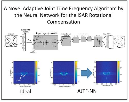
A Novel Adaptive Joint Time Frequency Algorithm by the Neural Network for the ISAR Rotational Compensation

Abstract

We propose a novel adaptive joint time frequency algorithm combined with the neural network (AJTF-NN) to focus the distorted inverse synthetic aperture radar (ISAR) image. In this paper, a coefficient estimator based on the artificial neural network (ANN) is firstly developed to solve the time-consuming rotational motion compensation (RMC) polynomial phase coefficient estimation problem. The training method, the cost function and the structure of ANN are comprehensively discussed. In addition, we originally propose a method to generate training dataset sourcing from the ISAR signal models with randomly chosen motion characteristics. Then, prediction results of the ANN estimator is used to directly compensate the ISAR image, or to provide a more accurate initial searching range to the AJTF for possible low-performance scenarios. Finally, some simulation models including the ideal point scatterers and a realistic Airbus A380 are employed to comprehensively investigate properties of the AJTF-NN, such as the stability and the efficiency under different signal-to-noise ratios (SNRs). Results show that the proposed method is much faster than other prevalent improved searching methods, the acceleration ratio are even up to 424 times without the deterioration of compensated image quality. Therefore, the proposed method is potential to the real-time application in the RMC problem of the ISAR imaging.

1. Introduction

Inverse synthetic aperture radar (ISAR) images are the two-dimensional projection of the target radar echo and can offer sufficient target signatures, such as the target’s movement and the detection for non-cooperative maneuvering targets [1]. An ideal rotational movement of the maneuvering target is the principle of range-doppler (RD) algorithm over a given coherent processing interval (CPI). In the empirical scene, however, besides the translational motion part, movements of targets also consist of other complex disturbances, such as rolling, pitching and yawing, causing smearing and distortion of ISAR images [2]. Thus, the motion compensation algorithm needs to be considered as the first step of ISAR images. Even though many methods have been successfully applied to remove the translational motion by the translational motion compensation (TMC) [3,4,5], the remaining unexpected rotational motions of target still induces a bad deterioration in ISAR images. Therefore, the final rotational motion compensation (RMC) procedure matters a lot.

During the past few years, several methods have been proposed for the RMC problem. Different autofocus algorithms [6,7,8] have been introduced to solve this problem. Some works use the time-frequency analysis [9,10]. In these works, authors carefully choose a short coherent processing interval using the time-frequency analysis. During the selected CPI, the motion of target is stable and can be regarded as constant. It dramatically reduces the potential distortion and shows a good result of the ISAR. This technique, however, does not make full use of radar signal, resulting in the decreasing of the cross-range resolution. In order to overcome disadvantages of the time-frequency analysis, some researchers introduce the theory of compressed sensing into the ISAR images reconstruction [11,12,13,14], especially for removing the non-uniform rotational motion. These works construct a parametric sparse representation model for the ISAR signal matrix, where the basis matrix is constructed according to the target rotation rate. Some works show good RMC results for an aircraft with rotational acceleration [11,12,13]. In addition, some works also use the sparse distribution of scatterers to directly reconstruct a high resolution ISAR image [15,16,17] Furthermore, another motion compensation approach with the cubic-order processing procedure [18] is also an option. The compressed sensing and RID offer an excellent solution for the post processing of ISAR imaging, it, however, is an extremely time-consuming algorithm which is not suitable for the real-time application.

The adaptive joint time frequency (AJTF) is comprehensively discussed solving the RMC problem [19], in which authors proposed a compensation method based on the estimation of polynomial phase coefficients of the cross-range signal on a special range cell which contains the dominant scatterer of the target. It is a panacea of this problem, if enough coefficients are estimated. However, the original AJTF algorithm needs the exhaustive searching to optimize the cost function, which obviously is time-consuming, so, the particle swarm optimization (PSO) and the genetic algorithm (GA) have been used as an improvement of tje AJTF algorithm to reduce the computational complexity [20]. However, when facing huge scene, the PSO and GA are still not competent, thus researchers focus on direct calculation method. In 2016, the polynomial phase coefficients of AJTF are estimated by polynomial phase transform (PPT) introduced by [21]. PPT dramatically reduces the time-consumption, however, it still has possibility to further improve.

The process of estimation is, essentially, a parameter estimator for a sophisticated input signal. Due to the complexity of the problem and the number of parameters, traditional ways of signal processing cannot get an accurate estimation. Fortunately, with the development of computational capacity, the neural network (NN) becomes a possible solution by the automatically machine learning for difficult estimation problems. Scientists have proven that multi-layer feed-forward networks, with even only one hidden layer, can approximate any function and provide any desired accuracy [22]. The most common utility of artificial neural network (ANN) is directly learning top-layer features, such as the detection of buildings [23] and airport [24] in the image classification problem. Some works, instead of directly recognition, use ANN estimator to analyze parameters, like the frequency of the signal [25,26], which can be used as inputs for traditional processing methods. It gives us a new way to improve the AJTF, because the ANN has been proved to be an operative estimator from those previous works.

Different from previous works of the RMC problem, a coefficient estimator based on the ANN is developed to replace the searching processes of the AJTF, like the PSO or the GA, in the RMC problem. The training method, cost function and structure of the ANN are comprehensively discussed. Meanwhile, since the lack of enough preliminary data makes the training more challenging in the ISAR problem, we originally propose a method to generate training dataset by the ISAR signal model with randomly chosen motion characteristics. Prediction results of the ANN estimator is used to directly compensate distorted ISAR images. Under some circumstances of the bad ISAR image quality, it can provide a more accurate and narrow initial searching range for the AJTF with PSO (AJTF-PSO). The proposed method is called as the adaptive joint time frequency algorithm combined with the neural network (AJTF-NN). Finally, ideal point scatterers and an aircraft model with complex motion are used to verify the validity of the proposed method. Simulation results show that the proposed method is much more faster than other prevalent improved searching methods. It can be even up to 424 times than the AJTF-PSO, and 2.07 times than the AJTF with PPT (AJTF-PPT). The proposed method also shows strong stability under different complex motion and signal-to-noise ratios (SNRs). Therefore, the proposed method is useful to the real-time application in the RMC problem of the ISAR imaging.

The remainder of this paper is organized as follows. In Section 2, a brief discussion to the AJTF is presented. In Section 3, a fully connected neural network and the design of training dataset are introduced, and the procedure of the AJTF-NN is articulated. Simulation results of the ideal scatterers and a realistic aircraft model are employed to comprehensively investigate properties of the AJTF-NN, such as the stability to different scenarios, influence on SNR and compensated ISAR image quality in Section 4. Finally, Section 5 goes the conclusion.

2. Materials and Methods

2.1. Signal Model for AJTF

Before employing the adaptive joint time-frequency algorithm to carry out the motion compensation, three basic assumptions are needed: (1) the target should be a rigid body during the CPI, i.e., the dominant scatterer contains motion characteristics of the whole target; (2) the target motion is confined to a 2-D plain, i.e., the target has only one fixed rotational axis in order to simplify the model and discussion of the RMC problem; (3) the coarse motion compensation, such as the range alignment, has been finished. Range alignment usually happens at the beginning of the ISAR imaging.

The following signal model is similar to those proposed in [19]. When all three assumptions are satisfied, the received radar signal in a chosen range cell can be written as,

$$s(f,t)=\sum _{k=1}^{N_k}{A}_{k}exp\left\{-\mathrm{j}\phi (f,t)\right\}$$

(1)

in which $N_k$ is the number of point scatterers within the range cell, t represents the slow time, $A_k$ is the power of the $k\mathrm{th}$ scatterer. In addition, the phase term $\phi (f,t)$ of the Equation (1) is,

$$\phi (f,t)=\frac{4\pi f}{c}\left(R\left(t\right)+x_{k}cos\left(\theta \left(t\right)\right)+y_{k}sin\left(\theta \left(t\right)\right)\right)$$

(2)

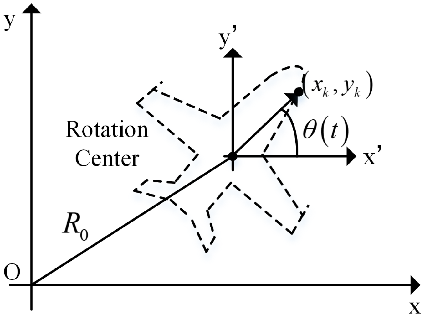
where f is the frequency, for the linear frequency modulation signal, and also represents the fast time, $(x_k,y_k)$ donates the $k\mathrm{th}$ scatterer position, range and cross range position, respectively. In Figure 1, $R_0$ is the distance between the radar antenna phase center and the center of the target, and $\theta \left(t\right)$ is the rotational motion. $R\left(t\right)$ is the residual uncompensated translational displacement . After the coarse range compensation, rotational motion phase term $\theta \left(t\right)$ has not improvement, and even though $R\left(t\right)$ will not exceed one range cell, it still will cause phase distortion which will lead to smearing. It can be expanded into polynomial functions of the dwelling time by Taylor series as,

$$\begin{array}{cc}\hfill R\left(t\right)& =R_0+V_{R}t+\frac{1}{2!}{V}_R^{\prime }{t}^2+\frac{1}{3!}{V}_R^{″}{t}^3\dots \hfill \\ \hfill \theta \left(t\right)& ={\theta }_0+\mathsf{\Omega }t+\frac{1}{2!}{\mathsf{\Omega }}^{\prime }{t}^2+\frac{1}{3!}{\mathsf{\Omega }}^{″}{t}^3\dots \hfill \end{array}$$

(3)

and substituting the Equation (3) into the Equation (2),

$$\begin{array}{l}\phi (f,t)=\frac{4\pi f}{c}[\left(R_0+V_{R}t+\frac{1}{2!}{V}_R^{\prime }{t}^2\right)\\ +x_{k}cos\left({\theta }_0+\mathsf{\Omega }t+\frac{1}{2!}{\mathsf{\Omega }}^{\prime }{t}^2\right)+y_{k}sin\left({\theta }_0+\mathsf{\Omega }t+\frac{1}{2!}{\mathsf{\Omega }}^{\prime }{t}^2\right)]\hfill \end{array}$$

(4)

and further expand the cos and sin in the Equation (4) and take the first three terms,

$$\begin{array}{cc}\hfill \phi \left(t\right)& =a_0+a_{1}t+a_2{t}^2\dots \hfill \\ \hfill a_0& =R_0+x_k\hfill \\ \hfill a_1& =V_R+y_k\mathsf{\Omega }\hfill \\ \hfill a_2& =\frac{1}{2}(V_R^{\prime }-x_k{\mathsf{\Omega }}^2+y_k{\mathsf{\Omega }}^{\prime })\hfill \end{array}$$

(5)

in which, $a_0$ donates the range position, $a_1$ contains the translational and rotational motion, which is necessary for the ISAR imaging. $a_2$ and high-order coefficients will cause the unexpected distortion if more complex motions exist. Thus, the purpose of motion compensation is eliminating phase terms of higher order (>2) and it can be solved by the adaptive joint time-frequency (AJTF) procedure.

The essential idea of the AJTF is finding the basis function which most resembles the Equation (1) on the dominant scatterer in the chosen range cell. The basis function is like,

$$h_p\left(t\right)=exp\left[-\mathrm{j}\frac{4\pi f_0}{c}\left(f_{1}t+\frac{1}{2}{f}_2{t}^2+\frac{1}{3}{f}_3{t}^3\dots \right)\right]$$

(6)

The best basis function is defined by a series of parameters which maximizes the similarity function,

$$\{f_1,f_2,f_3\dots \}=argmax\left[\frac{max\left(S\left(f\right){|}_x\right)}{{\sum }_x{S\left(f\right)|}_x}\right]$$

(7)

where, $S\left(f\right)$ is the power spectrum of the compensated signal. In order to speed the procedure, we use the power of fast fourier transform (FFT) of the compensated signal to estimate the power spectrum.

When the best basis function is successfully searched, for example ${\overline{h}}_p(t,f_{11},f_{12},f_{13},\dots )$, the residual uncompensated translational displacement $R\left(t\right)$ can be removed by the Equation (8),

$$\begin{array}{cc}\hfill s_c(f,t)& =s(f,t){\overline{h}}_p(t,f_{11},f_{12},f_{13},\dots )\hfill \\ & =\sum _{k=1}^{N_k}{A}_{k}exp\left\{-\mathrm{j}\frac{4\pi f_0}{c}\left[\Delta x_k+\Delta y_k\phi \left(t\right)\right]\right\}\hfill \end{array}$$

(8)

where $(\Delta x_k,\Delta y_k)$ is the differential position of the $k\mathrm{th}$ scatterer relative to the dominant point scatterer. After that, repeating the searching step for the compensated signal $s_c(f,t)$, we have the second best basis function whose parameters are $\{f_{21},f_{f22},f_{23},\dots \}$. We create a new dwelling time variable $t^{\prime }$, which is,

$$t^{\prime }=\frac{1}{f_{21}}(f_{22}{t}^2+f_{23}{t}^3+\dots )$$

(9)

Now, the rotational motion compensation can be eliminated using the linear interpolation on the new dwelling time $t^{\prime }$.

The searching of parameters set $\{f_{11},f_{12},f_{13},\dots \}$ is the key problem of the AJTF. Exhaustive searching is a trustworthy way for the optimal problem. However, a direct way to calculate the parameters set is urgently needed in the real-time application. The RMC problem can be transformed to a regression analysis one.

$$\mathbf{y}=s(\mathbf{t},f_{11},f_{12},f_{13},\dots )$$

(10)

Equation (10) is a regression model which relates the measured vector $\mathbf{y}$ to a function $\mathbf{t}$ and parameters $\{f_{11},f_{12},f_{13},\dots \}$. $s(\mathbf{t},f_{11},f_{12},f_{13},\dots )$ is a complex and non-uniform function, it, as a result, is difficult for traditional regression methods, like the linear regression and the ordinary least squares. However, the artificial neural network provides a powerful tool for the regression problem.

2.2. AJTF with Neural Network to the RMC

The artificial neural network is an ordinary feed-forward full-connected networks. However, the training dataset and combination of the AJTF are the key procedure as discussed in this section.

2.2.1. The Architecture

The neuron is the smallest unit of the neural network, and a typical multi-inputs multi-outputs neuron is expressed in the Equation (11).

$$a=f(\mathbf{wx}+b)$$

(11)

The vector $\mathbf{x}=\{x_1,\dots ,x_n\}$ is inputs of the neuron, and $\mathbf{w}$ is the corresponding weight vector. After influenced by bias b, the sum is passed to the activation function. Weight and bias define the performance of the neural network, thus, an optimal set of them is the goal of training the neural network, which is defined by the cost function.

For supervised learning, the optimal neural network has the lowest value of the cost function L, which measures the distance between the predicted output of the current network and the target output. Common cost functions contain the quadratic cost (mean squared error), the cross-entropy cost and the exponential cost etc. In this paper, for the regression problem, the mean squared error is used [27], which is,

$$L=\frac{1}{2}\sum _{m=0}^M{(t_m-a_m)}^2$$

(12)

where, $t_m$ is the $m\mathrm{th}$ target label value, $a_m$ is the corresponding output of the network, M is the number of the output.

Once the cost function L is determined, finding a series of weights $\mathbf{w}$ which minimizes the chosen function L is the main task. The gradient descent algorithms attempt to optimize the cost function L by following the steepest descent direction,

$$w_i=w_i-\eta \frac{\partial L}{\partial w_i}$$

(13)

in which, $\eta$ is the learning rate which controls how large of a step to take in the direction of the negative gradient. It is referred to as stochastic gradient descent (SGD). For SGD, however, the learning rate needs carefully set. A higher learning rate causes the network diverge, on the other hand, a lower one results in slow learning. Thus, we choose an ADADELTA optimizer [28] which can dynamically choose the learning rate during iterations. In addition, it also has some benefits, especially the robust to noise which is common in the ISAR imaging.

Dislike weights and biases which is generated automatically, the activation function needs carefully to be chosen. ReLUs [29] is now widely used in the neural network, because, comparing to common activation functions like the sigmoids and the hyperbolic tangents, it allows for faster and effective training of the neural structure on the large and complex dataset and also provides efficient computation [30].

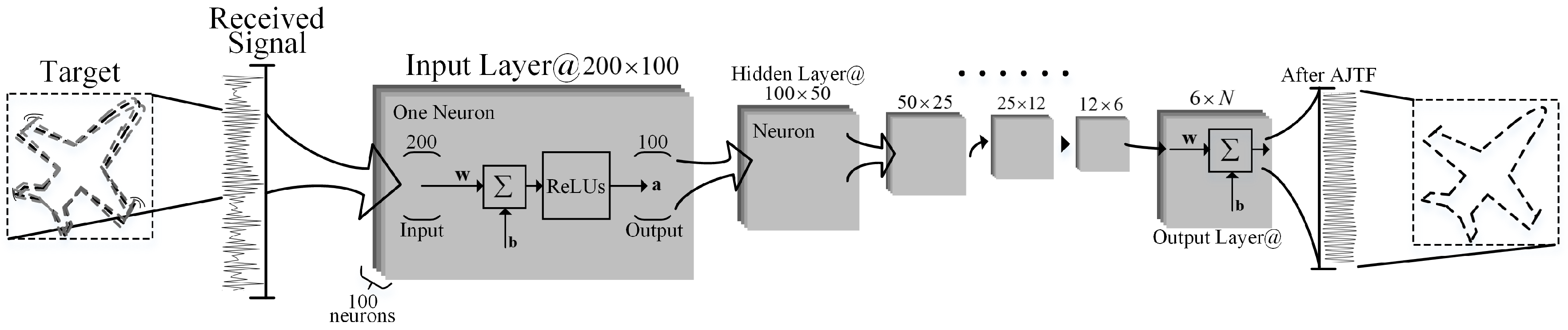
The architecture of the proposed neural network is an easy-to-employing feed-forward full-connected one, showing in Figure 2. The number of inputs of every neuron in the input layer is identical to the length of the signal. The mode of radar system is predestined, thus several neural networks with the different length of input layer are required to be trained. This setup is proper, because the length of signal only influences the sampling rate and the imaging time, and the radar signal model and the proposed line of thought are still valid. By changing the number of inputs of the proposed network, it can adapt to different radar systems. In following simulations, we set the number of inputs as 200. The deeper the network, the more accuracy regression results. In order to minimize the calculation load, the number of neurons in the hidden layer is tapered. In the end, at the output layer, we rescind the activation function to give maximum output range. The architecture is realized in the TensorFlow [31], which is deveopled by Google.

2.2.2. Training Datasets

The architecture of neural network influences a lot on the success of regression. Nevertheless, the overall success of the neural network regressor depends mostly on the training dataset. The NN-based method requires a large amount of training samples, however, in most circumstance, adequate samples are impossible to get. For example, it is impossible to obtain enough radar signal with different target motion characteristics and precisely measured trajectory path. Instead of training an end-to-end neural network, like in work [32], the training dataset is generated for a network who can estimate the polynomial coefficient, like in Equation (10). Thus the training dataset of the proposed method is generated by computer from a basic equation and a series of random chosen parameters. The basic equation of dataset is like the Equation (14).

$$h_b\left(t\right)=exp\left[-\mathrm{j}\frac{4\pi f_0}{c}\left(f_{1}t+\frac{1}{2}{f}_2{t}^2+\frac{1}{3}{f}_3{t}^3\dots \right)+2\pi N(0,1)\right]+n\left(t\right)$$

(14)

where, $N(0,1)$ is zeros means, unity variance Gaussian random variable, which provide a random initial phase and $n\left(t\right)$ is the additive noise. Other parameters of the Equation (14) are randomly chosen and corresponding sampling data of this Equation needs to be saved. Before the generation, two things need to be discussed: (1) the characteristics of polynomial coefficients, like the number and the value range; (2) the choice of the additive noise $n\left(t\right)$.

In the work of [21], for only acceleration existing, the author estimates only $f_1,f_2$ and achieves a good result of the RMC. For more complex scenario, like in the original work of Thayapara [19], a perturbed oscillation is added to the motion with a constant velocity, whose frequency is 1 Hz. The disturbed phase term is

$$\begin{array}{cc}\hfill {\phi }_d(f,t)& =A\left[x_{k}cos\left(p\left(t\right)\right)+y_{k}sin\left(p\left(t\right)\right)\right]\hfill \\ \hfill p\left(t\right)& =bsin\left(2\pi t\right)+\omega t\hfill \end{array}$$

(15)

in which, $A=4\pi f/c$, $R\left(t\right)$ is ignored in order to reduce the analysis, $\omega$ is the constant rotational motion and b is attenuation ratio which controls the influence of the perturbed oscillation, the subscript d means disturbed in order to distinguish with $\phi (f,t)$ in the Equation (4). The term inside the $exp\left(\right)$ of the Equation (8) is the Taylor expansion of $\phi (f,t)$, thus the determination of number of polynomial coefficients of the Equation (8) is to determine which order of $\phi (f,t)$ is too small to be ignore. Due to the fact that even under the circumstance with more severe smearing the ratio of oscillation b is still small. $p\left(t\right)$ is small enough during the dwelling time, thus we have approximation: $cos\left(p\right(t\left)\right)\approx 1,sin\left(p\right(t\left)\right)\approx p\left(t\right)$, then,

$${\phi }_d(f,t)=A\left[x_k+y_{k}bsin\left(2\pi t\right)+y_k\omega t\right]$$

(16)

After Jacobi-Anger expansion, we convert the Equation (15) to,

$$\begin{array}{cc}\hfill {\phi }_d(f,t)& =A{x}_k\sum _{n=-\infty }^{\infty }{J}_n\left(b\right)cos(2\pi nt+\omega t)\hfill \\ & +A{y}_k\sum _{n=-\infty }^{\infty }{J}_n\left(b\right)sin(2\pi nt+\omega t)\hfill \end{array}$$

(17)

where, $J_n\left(b\right)$ is the $n\mathrm{th}$ Bessel function of the first kind. The fourth order coefficient, contributed by cos part, is small enough to be ignored. Thus, the final training dataset contains only the first three orders $f_1,f_2,f_3$. The range of $f_1,f_2,f_3$ is determined by the scene size, in other words, the Doppler bandwidth which is limited by the pulse repeat frequency. Hence, the range of $f_1,f_2,f_3$ is $(-N,N)$, N is the pulse repeat frequency. The pulse repeat frequency of one radar image system will determinate the largest doppler of it, in other words, the range of cross dimension. Thus, if in the real data some parameters aren’t contained in our dataset, the radar image has been aliased in cross range which should be avoided when we try to use radar to image remote targets.

As for the choice of $n\left(t\right)$, it depends on the environment where the target is. When ISAR oversees a target in the air, $n\left(t\right)$ only contains the additive white Gaussian noise (AWGN) led by the radar receiver. The overall size of training dataset is 20,000. It is not the larger the better. Work [33] has proved that stopping of neural network training before overfitting allows significant increasing of neural network predictive performance for test datasets in comparison to that of overtrained networks. Thus, 20,000 times is a suggested number of training iteration. By the data discussed above, the proposed neural network is trained. The value of the cost function in the end training is less than 2, which means that the proposed network is convergent and will have a good prediction performance.

2.2.3. Procedure of AJTF with Neural Network

The first step of AJTF-NN is the choosing of the dominant scatterer. The range cell which contains the dominant scatterer has the highest signal-to-noise ratio (SNR) and full movement characteristics based on rigid body assumption. The way of determination of the dominant scatterer place is amplitude normalized variance (ANV) [21]. The definition of the $n\mathrm{th}$ range cell is,

$${\sigma }_n=1-\frac{E\left(\right|s(f,t_n){\left|\right)}^2}{E\left(\right|s(f,t_n){|}^2)}$$

(18)

where E is the expectation. The dominant scatterer has the most possibility in the range cell whose ${\sigma }_n$ is relatively small. By chosing the range cell with a dominant scatterer, it avoid the false estimation of the neural network when predicting a cell has two or more scatterers whose RCSs are near. In addition, the training dataset contains noise factor which give him the ability to overcome the disturb led by minor scatterers.

After the range cell is chosen, the proposed neural network is applied to predict coefficients of the target image and the whole ISAR image is compensated by these coefficients based on the method discussed in Section 2. Even though the final cost of prediction is small, images compensated by this series of coefficients may still have smearing if the higher order estimated coefficient contributes more on the cost. A further compensation is needed if the ISAR image quality is lower. A common image quality assessment is peak-sublobe ratio (PSLR),

$$Q_{PSLR}=\frac{|S\left(f_{peak}\right){|}^2}{{\sum \left|S\left(f\right)\right|}^2}$$

(19)

where $S\left(f\right)$ is the power spectrum evaluated by FFT and $f_{peak}$ is the peak frequency. It is the power of the peak in frequency domain against the whole power in one range cell [34]. Based on the ISAR RD imaging principle, the frequency is proportional to the cross range. Thus the more power of the peak in total power, the more focused in ISAR image. If the PSLR of compensated image is larger than a threshold $\delta$ (depending on the usage of the ISAR image, 0.6 is chosen as an example in the proposed scenario), there is no need to further compensate. If not, a fine compensation should be applied by AJTF-PSO, whose searching range is significantly shrunk by the prediction of the proposed neural network. This fine compensation may lead to more computational load. However, as the analysis discussed in following section shows, under most circumstances, there is no need of fine compensation and it has few influence on the overall consumption. By this technique, the harmony between the quality and computation load is achieved.

The AJTF-NN is comprehensively listed in the Algorithm 1.

Algorithm 1 AJTF-NN

Require: The ISAR signal matrix $s(f,t)$, and trained neural network

(Select the range cell with the dominant scatter).

for $i=0$ to N do

Calculate ANV for every range cell

$M\leftarrow {\sigma }_i$

end for

Sort the smallest ANV and corresponding position n, ${\sigma }_{min}\leftarrow M$

$\{f_1,f_2,f_3\}=NN\leftarrow s(f,nT)$ (Put the dominent range cell into trained neural network)

$s_c(f,nT)\stackrel{RMC}{\leftarrow }{s}_t(f,nT)\stackrel{TMC}{\leftarrow }s(f,nT)$

$Q_{PSLR}\leftarrow s_c(f,nT)$

if $Q_{PSLR}>\delta$ then

image quality is good enough

else

image quality is not good enough

$\{f_{1n},f_{2n},f_{3n}\}\leftarrow PSO-AJTF\leftarrow \{f_1,f_2,f_3\}$

$\{f_1,f_2,f_3\}\leftarrow \{f_{1n},f_{2n},f_{3n}\}$

end if

for $i=0$ to N do

$s_c(f,iT)\stackrel{RMC}{\leftarrow }{s}_t(f,iT)\stackrel{TMC}{\leftarrow }s(f,iT)$

end for

The algorithm does not need iteration, the computation complexity of this proposed method is $T\left(n\right)=O\left(n\right)$. Thus, AJTF-NN can directly and fast compensate the ISAR image. It is much swifter than other AJTF methods, such as AJTF-PSO of its complexity $O\left(n^2\right)$. By the given training dataset and architecture, it requires aproximately 1 h to train the proposed neural network. However, when estimating the overall performance of AJTF-NN, the training time should not be considered [24,35], because the training is a preliminary step, it can be done before processing ISAR image. Thus, the AJTF-NN is a swift and efficient method.

3. Results

In this section, we present some simulation results to investigate the proposed method. All results are generated and run on a personal computer consisting of Core i7-4760 with 4 processors at 3.6 GHz. Two models are used: (1) ideal point scatterers, (2) airbus A380 model.

3.1. Ideal Point Scatterers

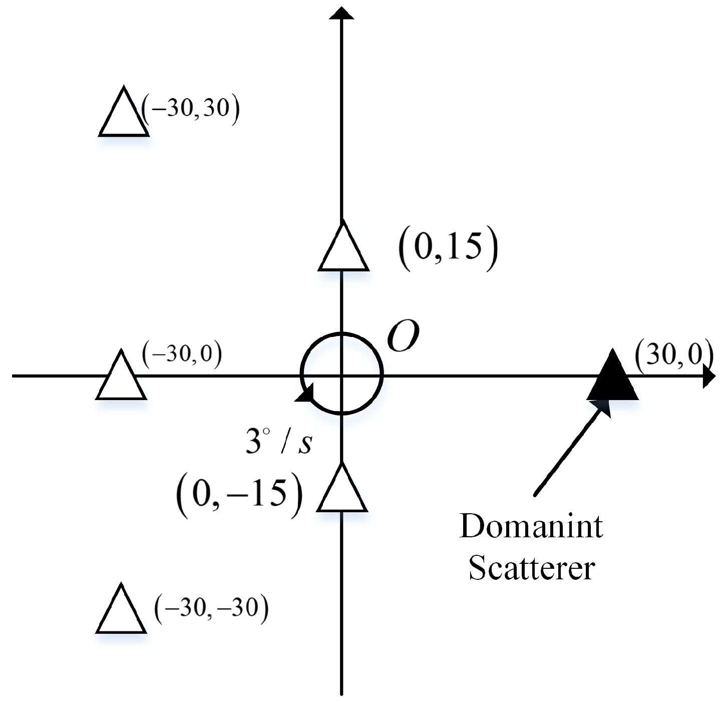
The ideal point scatterers model derives from the model of original work of Thayaparan [19]. It contains 6 corner reflectors and is uniformly rotating at a constant rate of 3${}^{\circ }/\mathrm{s}$, anti-clockwise (see details in Figure 3. In addition, the solid black corner reflector is intentionally set as the dominant scatterer whose radar cross section (RCS) is larger than others. In addition, simulation parameters of the ISAR are listed in

Table 1. Simulation Parameters of ISAR.

Name of the Paramter	Value
Carrier frequency	$9.05\mathrm{GHz}$
Bandwidth	$75\mathrm{MHz}$
CPI	$100\mathrm{ms}$
Number of range cells	100
Number of cross-range Cells	100

. Three properties of the AJTF-NN need comprehensive discussions, (1) image results, (2) efficiency and (3) stability.

3.1.1. Image Results

By this deployment of the ISAR, Figure 4a shows the ISAR image without distortion, clearly focusing every point of corner reflector. Adding yawing with frequency for $0.5\mathrm{Hz}$ into the uniform rotation, see in Figure 4b, as a comparison, the figure shows that the image is severely distorted in cross-range dimension. The Figure 4c,d are the compensated image processed by AJTF-NN and original AJTF, respectively. The AJTF-NN almost has the same performance as the original AJTF. Both of them perfectly eliminate the blur of image and the $Q_{PSLR}$s of dominant scatterer are $0.6265$ and $0.6965$, respectively, comparing to the $Q_{PSLR}$ of Figure 4a $0.7314$. In addition, images processed by AJTF-PPT and AJTF-PSO are also shown in Figure 4d,e, respectively as a comparison. The AJTF-NN almost has the same performance as the improved AJTF methods. Far more analysis to illustrate the difference will be done in following section by the numerical simulation.

3.1.2. Efficiency

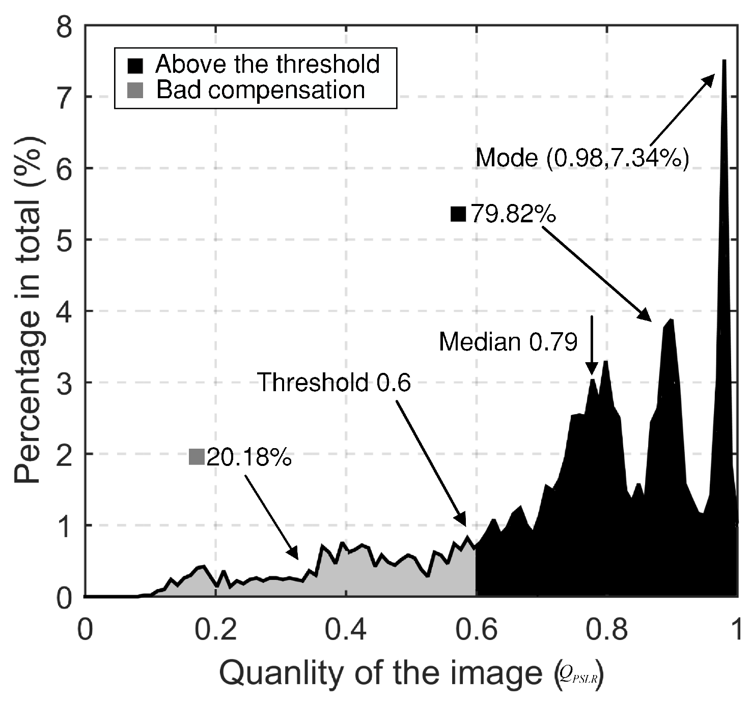
The most appealing characteristic of the AJTF-NN is its efficiency. As discussed in the Section 2.2.3, a fine compensation finished by the AJTF-PSO is needed to provide a constant high image quality when the image quality defined by $Q_{PSLR}$ is lower than 0.6. To show the influence of it, we execute Monte Carlo simulation for 5000 times with different circumstances. The non-uniform motion is led by the acceleration which is randomly chosen from $1^{\circ }/{\mathrm{s}}^2$ to ${10}^{\circ }/{\mathrm{s}}^2$. The statistic results of the Monte Carlo simulation is illustrated in Figure 5, where the image quality distribution without the fine compensation is presented. When the fine compensation threshold of the AJTF-NN is set at 0.6 which is near the quality of Figure 4c, the AJTF-PSO does not need to get involved in $79.82\%$ processes. Thus, the fine compensation will not have a significant influence on the overall performance.

In addition, the overall performance are recorded during the Monte Carlo simulation with other three AJTF algorithms (AJTF-PSO, AJTF-PPT and Traditional AJTF). The averaged computational time is listed in

Table 2. Computational Time of Different RMC Algorithms.

Method Name	Computational Time (s)
	Only Estimation	Whole Compensation
Traditional AJTF	$0.5947$	$0.6047$
AJTF-PSO	$0.1902$	$0.2030$
AJTF-PPT	$0.0029$	$0.0164$
AJTF-NN	$0.0014$	$0.0145$

. In Table 2, the time used by the estimation step is separately listed, because the compensation step consumption is the same for all four algorithms, which is approximate $10\mathrm{ms}$. Results show that the AJTF-NN is much faster than other prevalent improved searching methods, the acceleration ratio are even up to 424, 2.07 times than the AJTF-PSO and the AJTF-PPT respectively without the deterioration of the compensated image quality. The estimation step contributes most on the difference, thus when ISAR is watching more than one targets the AJTF-NN will have more advantages.

3.1.3. Stability

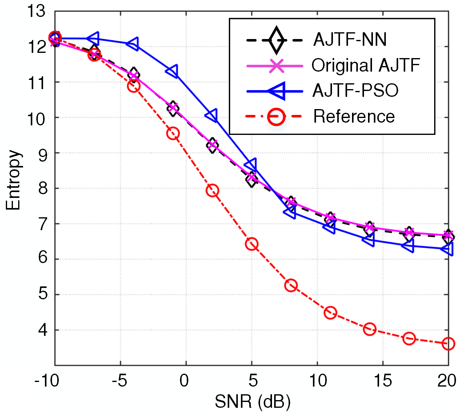
We analyzed the influence of the noise on the performance of the AJTF-NN. Image entropy is used to reflect the property, which is

$$\begin{array}{c}E=-\sum _{n=0}^{N-1}\sum _{m=0}^{M-1}\frac{{\left|I(m,n)\right|}^2}{S}ln\frac{{\left|I(m,n)\right|}^2}{S}\hfill \\ S=\sum _{n=0}^{N-1}\sum _{m=0}^{M-1}{\left|I(m,n)\right|}^2\hfill \end{array}$$

(20)

in which, $M,N$ are the number of pixel of X-axis and Y-axis, respectively, $I(m,n)$ is the ISAR image which is generated by the RD algorithm. The entropy is a measurement standard of unpredictability. With the decreasing of the SNR, the entropy raises. A picture with only white noise has the largest entropy. Because the entropy is not an absolutely standard for the ISAR image quality, the reference image is used (like Figure 4a) which does not contain any distortion to compare with the ISAR image compensated by the proposed method. The original AJTF and the AJTF-NN are carried out under different SNRs ranging from $-10\mathrm{dB}$ to $20\mathrm{dB}$, in which 50 Monte-Carlo simulations are conducted at each SNR. The simulation result is shown in Figure 6.

Even though the neural network is a nonlinear system, In this simulation, the AJTF-NN shows the same property as the original AJTF, which means that noise does not have a great influence on the proposed method. However, when the noise is small enough, the entropy led by distortion takes the dominant position. When the SNRs is worsen ($SNR<0\mathrm{dB}$), the entropy of SAR image provided by the AJTF-NN is still at the same order. Thus, the stability of AJTF-NN under different circumstances is guaranteed.

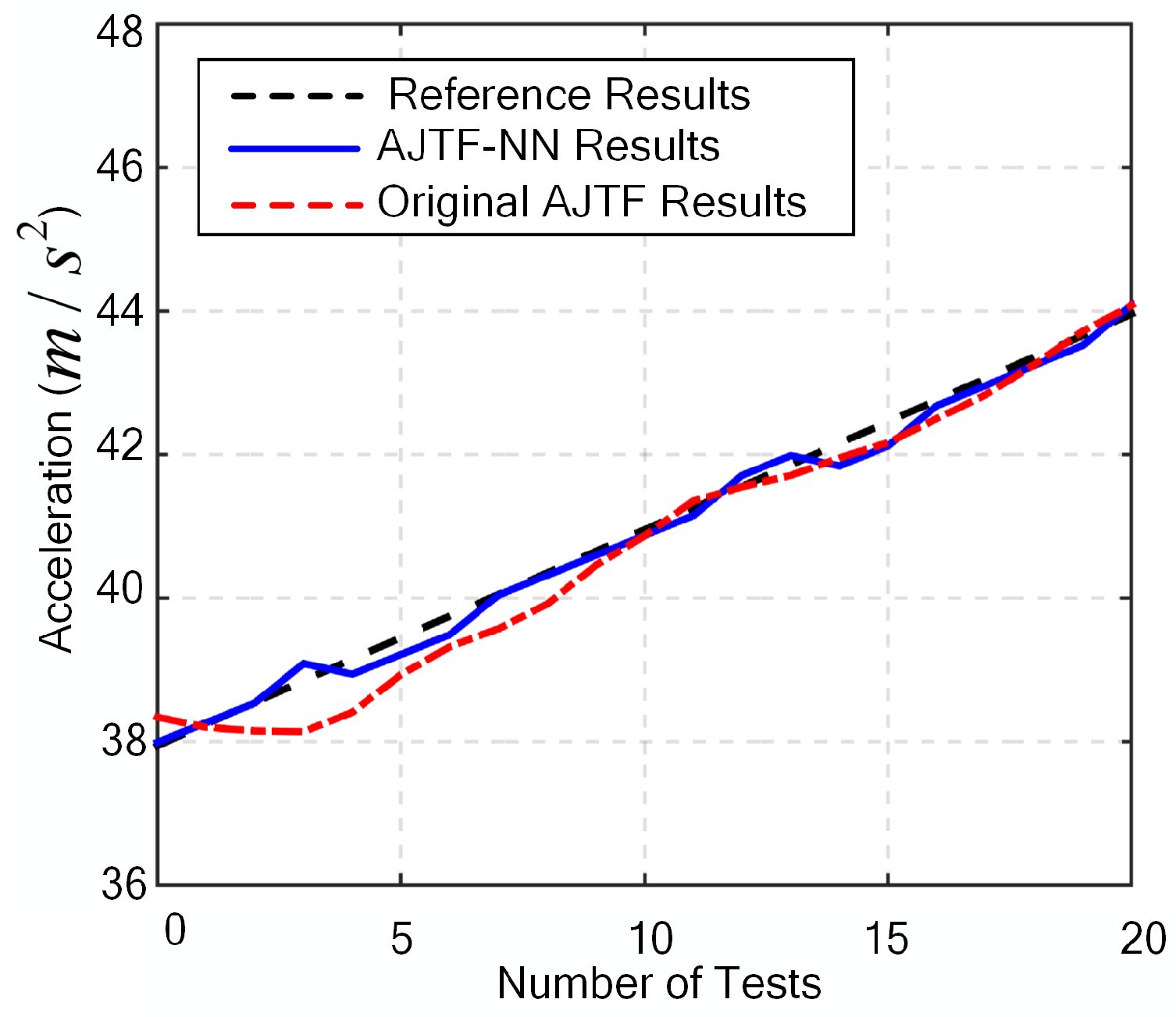
In addition, based on the relationship between the estimated coefficients and simulation parameters in the Equation (5), parameters can be calculated, like acceleration of the target, from the output of the AJTF-NN. We give the result of estimated parameters by the AJTF-NN to show the accuracy. The acceleration estimation results by AJTF-NN is in Figure 7.

In Figure 7, the AJTF-NN shows a good result, even though under some circumstances the maximum error is approximately $2\mathrm{m}/{\mathrm{s}}^2$.

3.2. Airbus A380

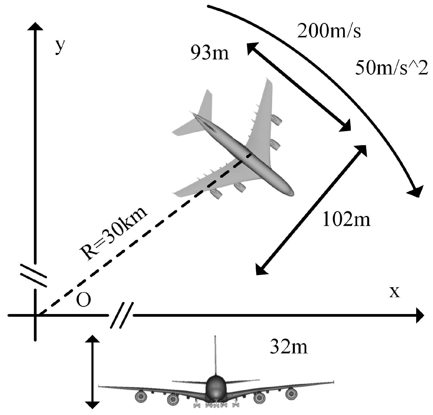
As a more realistic simulation, a full size Airbus A380 aircraft with dimensions which are about length of $93\mathrm{m}$, width of $102\mathrm{m}$ and height of $32\mathrm{m}$ is employed to test the capability of the proposed method. As shown in Figure 8, the cruise speed of flight is set as $200\mathrm{m}/\mathrm{s}$. The distance between the antenna phase center of the radar and the center of airplane is $30\mathrm{km}$. The required radar data are obtained by a trustworthy electromagnetic (EM) scattering solver, shooting and bouncing rays (SBR) [36], which is widely used to generate the radar scattering echo of an electrically large scale target. The horizontal-horizontal polarized mono-static scatterings are generated and collected by this EM solver. In addition, the simulation parameters of the ISAR are listed in Table 1, except the bandwidth is changed to $300\mathrm{MHz}$.

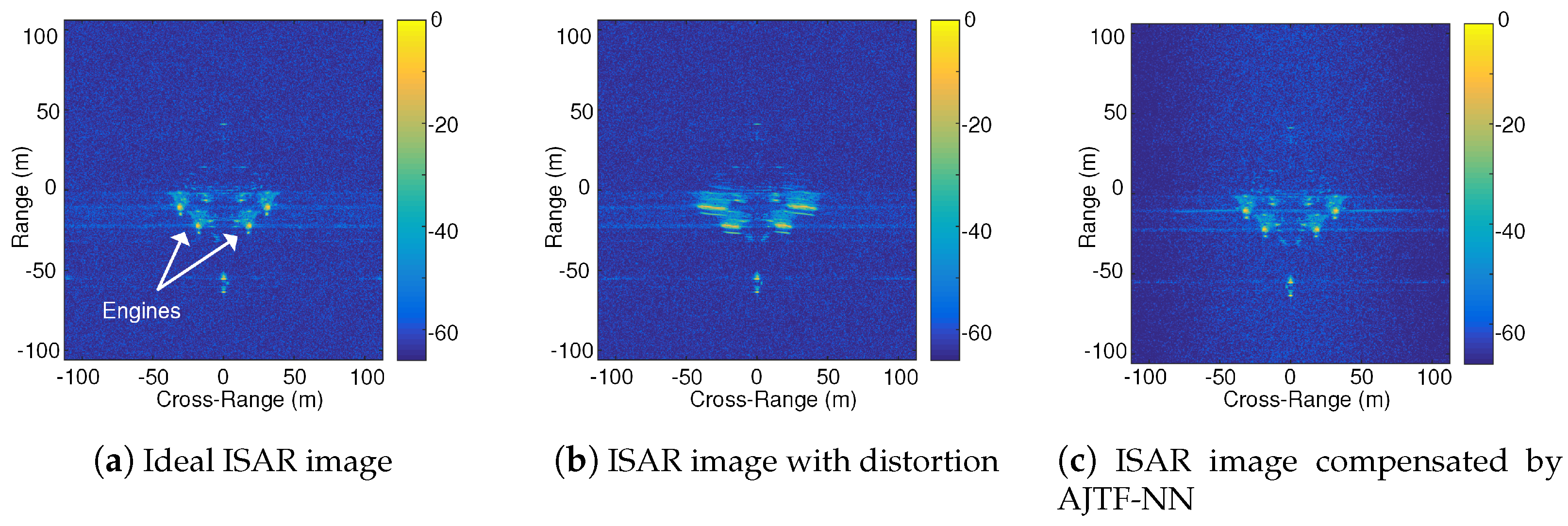
The Figure 9a is an ideal A380 ISAR image with these parameters, in which, several key structures like four engines and the outline of A380 are clearly illustrated (the white line in Figure 9a is the outline of the model). Engines of aircraft usually have stronger scatterings than the other parts due to its cone structure, and are the most interesting components for ISAR recognition algorithm.

Figure 9b shows the ISAR image of the Airbus A380 with distortion. The distortion in this image is led by a yew with $0.5\mathrm{Hz}$. In the cross-range, because the image is highly fuzzy, the outline of the A380 is covered by the spread of the power and the position of engines is hard to determine. Thus, it results in great difficulties of radar detection and recognition. After handled by the AJTF-NN, in Figure 9c, the surrounding area of the ISAR image is adequately sharp. The image quality $Q_{PSLR}$ of Figure 9c is $0.6124$, and as a comparison, the image quality of Figure 9a is $0.6398$. The time consumption of the AJTF-NN when process the A380 model is $3.9072\mathrm{s}$. It differs from ideal scatterers model because the scene of A380 is much larger with a higher image resolution. The time consumption of the original AJTF is $37.52\mathrm{s}$. It has proven that the AJTF-NN is more efficient to handle more general and complex rotational motion compensation problems in the ISAR imaging.

4. Discussion

The strength of the proposed method lies in the efficiency when a good image compensation result is guaranteed, as shown in Figure 4 and Table 2. The training time is the main problem of the proposed method. There are several novel and cutting-edge papers [14,15,17] which reconstruct ISAR image from rotational movement by compressed sensing. Comparing to the result of these papers, when considering the training time, which will take about 1 h or longer, the proposed method is not efficient. However, the training procedure is a preliminary step. It will be done before it is applied to compensate radar image. For example, in other neural network related papers [24,35,37], they do not consider the training time when listing total performance. Thus, the time consumption of training procedure should not be considered in the total performance.

Furthermore, the training parameters will change under different mode of radar system. However, it will only influence the sampling rate and imaging time, thus the radar signal model and the proposed line of thought are still valid. By changing the number of inputs of the proposed network, it can adapt to different radar systems.

The image compensation performance of proposed method, as shown in the Section 3.2 is almost similar to the conventional AJTF. The justification of having a new method is based on two following reasons. First, the conventional AJTF, which uses an exhaust searching estimation method, will always find the optimal solution in the given range. In order words, the conventional AJTF will have the best performance. Thus, if the proposed method could have the same image compensation quality, which surely have, as shown in the Section 3.2, the proposed method is good enough considering the compensation performance. Secondly, even though the conventional AJTF has the best solution, the time-consumption of it is intolerable employing for the real-time imaging. Thus when considering the performance of the time-consumption, the proposed method has a considerable advantage comparing to the other AJTF methods. Combining these two reasons, the proposed method, which provides the same image compensation quality and is efficient, is a novel AJTF method.

5. Conclusions

In this paper, we propose a novel adaptive joint time frequency algorithm combined with neural network (AJTF-NN) to focus the distorted the inverse synthetic aperture radar (ISAR) image when the target is in rotational motion, and a coefficient estimator based on the artificial neural network (ANN) is developed to solve the time-consuming problem in the rotational motion compensation (RMC) polynomial phase coefficient estimation. Comparing to the traditional AJTFs, the AJTF-NN is a more efficient method which can reduce greatly the computational cost. Some simulations have illustrated the stability and efficiency of the AJTF-NN under different SNRs. In addition, a realistic Airbus A380 model based on EM simulation also supports that the AJTF-NN is qualified for more complex circumstances. Thus, the AJTF-NN has a great potential in ISAR image compensation problems.

Some possible extensions of this method should include a refinement of the neural network architecture which will lead to a less computational cost and training time, or a refinement of training dataset for other complex scenarios, such as the ship-ocean problem.

References

- Ozdemir, C. Inverse Synthetic Aperture Radar Imaging with MATLAB Algorithms; John Wiley & Sons: Hoboken, NJ, USA, 2012; Volume 210. [Google Scholar]
- Chen, V.C.; Lipps, R. ISAR imaging of small craft with roll, pitch and yaw analysis. In Proceedings of the Record of the IEEE 2000 International Radar Conference, Alexandria, VA, USA, 12 May 2000; pp. 493–498. [Google Scholar]
- Yu, Z.; Wang, S.; Li, Z. An imaging compensation algorithm for spaceborne high-resolution SAR based on a continuous tangent motion model. Remote Sens. 2016, 8, 223. [Google Scholar] [CrossRef]
- Zhang, S.; Zhou, F.; Sun, G.C.; Xia, X.G.; Xing, M.D.; Bao, Z. A New SAR–GMTI High-Accuracy Focusing and Relocation Method Using Instantaneous Interferometry. IEEE Trans. Geosci. Remote Sens. 2016, 54, 5564–5577. [Google Scholar] [CrossRef]
- Wang, J.; Liu, X.; Zhou, Z. Minimum-entropy phase adjustment for ISAR. IEEE Proc. Radar Sonar Navig. 2004, 151, 203–209. [Google Scholar] [CrossRef]
- Kang, B.S.; Kang, M.S.; Choi, I.O.; Kim, C.H.; Kim, K.T. Efficient Autofocus Chain for ISAR Imaging of Non-Uniformly Rotating Target. IEEE Sens. J. 2017, 17, 5466–5478. [Google Scholar] [CrossRef]
- Wu, C.; Wang, H.; Deng, B.; Qin, Y.; Su, W. Autofocus technique for ISAR imaging of uniformly rotating targets based on the ExCoV method. J. Syst. Eng. Electron. 2017, 28, 267–275. [Google Scholar] [CrossRef]
- Xu, J.; Cai, J.; Sun, Y.; Xia, X.G.; Farina, A.; Long, T. Efficient ISAR Phase Autofocus Based on Eigenvalue Decomposition. IEEE Geosci. Remote Sens. Lett. 2017, 14, 2195–2199. [Google Scholar] [CrossRef]
- Hu, C.; Ferro-Famil, L.; Kuang, G. Ship discrimination using polarimetric SAR data and coherent time-frequency analysis. Remote Sens. 2013, 5, 6899–6920. [Google Scholar] [CrossRef] [Green Version]
- Qian, S.; Chen, D. Decomposition of the Wigner-Ville distribution and time-frequency distribution series. IEEE Trans. Signal Process. 1994, 42, 2836–2842. [Google Scholar] [CrossRef]
- Khwaja, A.S.; Zhang, X.P. Compressed sensing ISAR reconstruction in the presence of rotational acceleration. IEEE J. Sel. Top. Appl. Earth Observ. Remote Sens. 2014, 7, 2957–2970. [Google Scholar] [CrossRef]
- Rao, W.; Li, G.; Wang, X.; Xia, X.G. Adaptive Sparse Recovery by Parametric Weighted L1 Minimization for ISAR Imaging of Uniformly Rotating Targets. IEEE J. Sel. Top. Appl. Earth Observ. Remote Sens. 2013, 6, 942–952. [Google Scholar] [CrossRef]
- Rao, W.; Li, G.; Wang, X.; Xia, X.G. Parametric sparse representation method for ISAR imaging of rotating targets. IEEE Trans. Aerosp. Electron. Syst. 2014, 50, 910–919. [Google Scholar] [CrossRef]
- Chen, Y.C.; Li, G.; Zhang, Q.; Zhang, Q.J.; Xia, X.G. Motion compensation for airborne SAR via parametric sparse representation. IEEE Trans. Geosci. Remote Sens. 2017, 55, 551–562. [Google Scholar] [CrossRef]
- Wang, B.; Zhang, S.; Wang, W.Q. Bayesian inverse synthetic aperture radar imaging by exploiting sparse probing frequencies. IEEE Antennas Wirel. Propag. Lett. 2015, 14, 1698–1701. [Google Scholar] [CrossRef]
- Khwaja, A.S.; Cetin, M. Compressed Sensing ISAR Reconstruction Considering Highly Maneuvering Motion. Electronics 2017, 6, 21. [Google Scholar] [CrossRef]
- Zhao, L.; Wang, L.; Bi, G.; Yang, L. An autofocus technique for high-resolution inverse synthetic aperture radar imagery. IEEE Trans. Geosci. Remote Sens. 2014, 52, 6392–6403. [Google Scholar] [CrossRef]
- Zheng, J.; Su, T.; Zhu, W.; Zhang, L.; Liu, Z.; Liu, Q.H. ISAR imaging of nonuniformly rotating target based on a fast parameter estimation algorithm of cubic phase signal. IEEE Trans. Geosci. Remote Sens. 2015, 53, 4727–4740. [Google Scholar] [CrossRef]
- Thayaparan, T.; Lampropoulos, G.; Wong, S.; Riseborough, E. Application of adaptive joint time–frequency algorithm for focusing distorted ISAR images from simulated and measured radar data. IEEE Proc. Radar Sonar Navig. 2003, 150, 213–220. [Google Scholar] [CrossRef]
- Brinkman, W.; Thayaparan, T. Focusing ISAR images using the AJTF optimized with the GA and the PSO algorithm-comparison and results. In Proceedings of the 2006 IEEE Conference on Radar, Verona, NY, USA, 24–27 April 2006. [Google Scholar]
- Kang, B.S.; Bae, J.H.; Lee, S.J.; Kim, C.H.; Kim, K.T. Isar rotational motion compensation algorithm using polynomial phase transform. Microw. Opt. Technol. Lett. 2016, 58, 1551–1557. [Google Scholar] [CrossRef]
- Hornik, K.; Stinchcombe, M.; White, H. Multilayer feedforward networks are universal approximators. Neural Netw. 1989, 2, 359–366. [Google Scholar] [CrossRef]
- Maggiori, E.; Tarabalka, Y.; Charpiat, G.; Alliez, P. Convolutional neural networks for large-scale remote-sensing image classification. IEEE Trans. Geosci. Remote Sens. 2017, 55, 645–657. [Google Scholar] [CrossRef]
- Cai, B.; Jiang, Z.; Zhang, H.; Zhao, D.; Yao, Y. Airport Detection Using End-to-End Convolutional Neural Network with Hard Example Mining. Remote Sens. 2017, 9, 1198. [Google Scholar] [CrossRef]
- Alavi, H.; Fadaei, M. Frequency estimation of low rate non-uniformly sampled signals using neural networks. In Proceedings of the IEEE Singapore ICCS’94 Conference, Singapore, 14–18 November 1994; Volume 1, pp. 229–233. [Google Scholar]
- Tóth, B.P.; Csapó, T.G. Continuous fundamental frequency prediction with deep neural networks. In Proceedings of the IEEE 2016 24th European Signal Processing Conference (EUSIPCO), Budapest, Hungary, 29 August–2 September 2016; pp. 1348–1352. [Google Scholar]
- Bishop, C.M. Pattern Recognition and Machine Learning; Springer: New York, NY, USA, 2006. [Google Scholar]
- Zeiler, M.D. ADADELTA: An Adaptive Learning Rate Method. arXiv, 2012; arXiv:1212.5701. [Google Scholar]
- Nair, V.; Hinton, G.E. Rectified linear units improve restricted boltzmann machines. In Proceedings of the 27th International Conference on Machine Learning (ICML-10), Haifa, Israel, 21–24 June 2010; pp. 807–814. [Google Scholar]
- Glorot, X.; Bordes, A.; Bengio, Y. Deep sparse rectifier neural networks. In Proceedings of the Fourteenth International Conference on Artificial Intelligence and Statistics, Fort Lauderdale, FL, USA, 11–13 April 2011; pp. 315–323. [Google Scholar]
- Abadi, M.; Agarwal, A.; Barham, P.; Brevdo, E.; Chen, Z.; Citro, C.; Corrado, G.S.; Davis, A.; Dean, J.; Devin, M.; et al. TensorFlow: Large-Scale Machine Learning on Heterogeneous Distributed Systems. 2015. Available online: download.tensorflow.org/paper/whitepaper2015.pdf (accessed on 23 February 2018).
- Tatarchenko, M.; Dosovitskiy, A.; Brox, T. Multi-view 3d models from single images with a convolutional network. In European Conference on Computer Vision; Springer: Cham, Switzerland, 2016; pp. 322–337. [Google Scholar]
- Tetko, I.V.; Livingstone, D.J.; Luik, A.I. Neural network studies. 1. Comparison of overfitting and overtraining. J. Chem. Inf. Comput. Sci. 1995, 35, 826–833. [Google Scholar] [CrossRef]
- Jung, C.H.; Jung, J.H.; Oh, T.B.; Kwag, Y.K. SAR image quality assessment in real clutter environment. In Proceedings of the 2008 7th European Conference on Synthetic Aperture Radar (EUSAR), Friedrichshafen, Germany, 2–5 June 2008; pp. 1–4. [Google Scholar]
- Mou, L.; Ghamisi, P.; Zhu, X.X. Deep Recurrent Neural Networks for Hyperspectral Image Classification. IEEE Trans. Geosci. Remote Sens. 2017, 55, 3639–3655. [Google Scholar] [CrossRef]
- Yang, W.; Kee, C.Y.; Wang, C.F. Novel Extension of SBR-PO Method for Solving Electrically Large and Complex Electromagnetic Scattering Problem in Half-Space. IEEE Trans. Geosci. Remote Sens. 2017, 55, 3931–3940. [Google Scholar] [CrossRef]
- Xu, Z.; Xu, X.; Wang, L.; Yang, R.; Fangling, P. Deformable ConvNet with Aspect Ratio Constrained NMS for Object Detection in Remote Sensing Imagery. Remote Sens. 2017, 9, 1312. [Google Scholar] [CrossRef]
Figure 1.
Geometry of ISAR.
Figure 2.
Neural Network Architecture. (@ , for example, represents this layer has 200 inputs and 100 outputs).
Figure 3.
Geometry of the six corner reflectors (the solid black one is intentionally set as the dominant scatterer).
Figure 4.
ISAR simulations of ideal point scatterers @.
Figure 5.
Monte Carlo simulation of AJTF-NN @ 5000 times, .
Figure 6.
Performances of AJTF-NN with different SNRs.
Figure 7.
Comparison on estimated acceleration results.
Figure 8.
Geometry and dimension of Airbus A380.
Figure 9.
ISAR simulations of Airbus A380.