Spatio-Temporal Characterization of a Reclamation Settlement in the Shanghai Coastal Area with Time Series Analyses of X-, C-, and L-Band SAR Datasets

Abstract

Large-scale reclamation projects during the past decades have been recognized as one of the driving factors behind land subsidence in coastal areas. However, the pattern of temporal evolution in reclamation settlements has rarely been analyzed. In this work, we study the spatio-temporal evolution pattern of Linggang New City (LNC) in Shanghai, China, using space-borne synthetic aperture radar interferometry (InSAR) methods. Three data stacks including 11 X-band TerraSAR-X, 20 L-band ALOS PALSAR, and 35 C-band ENVISAT ASAR images were used to retrieve time series deformation from 2007 to 2010 in the LNC. An InSAR analysis from the three data stacks displays strong agreement in mean deformation rates, with coefficients of determination of about 0.9 and standard deviations for inter-stack differences of less than 4 mm/y. Meanwhile, validations with leveling data indicate that all the three data stacks achieved millimeter-level accuracies. The spatial distribution and temporal evolution of deformation in the LNC as indicated by these InSAR analysis results relates to historical reclamation activities, geological features, and soil mechanisms. This research shows that ground deformation in the LNC after reclamation projects experienced three distinct phases: primary consolidation, a slight rebound, and plateau periods.

1. Introduction

Reclamation is a potential solution to the growing demand for new land for living and development in cities. Over the past decades, the Netherlands, China, the UK, Japan, Singapore, and other coastal countries have extensively exploited sea enclosures and reclamation for coastal city development [1]. Because reclamation usually consists of dumping un-compacted filling materials over unconsolidated marine sediments, land subsidence has always been a significant issue in such areas, and could lead to damage to structures and poses a threat to public safety and the environment [2]. Therefore, it is crucial to monitor land subsidence in reclaimed areas to facilitate an understanding of the evolutionary processes so that proper measures can be taken to plan construction efficiently and mitigate loss.

Ground motion can be measured by geodetic techniques such as GPS or the leveling of specific targets. However, this task is labor-intensive and time-consuming, and more importantly, it can only provide discrete information at a limited number of points. In contrast to these traditional techniques, repeat-pass space-borne synthetic aperture radar (SAR) interferometry (InSAR) permits large-scale ground subsidence field retrieval without any prior knowledge, especially with the advent of time series InSAR analysis [3]. These advanced InSAR methods [4,5,6] are capable of estimating time series deformation through an analysis of phase signals over selected Coherent Points (CPs) and have become a mature tool for land subsidence monitoring in urban areas, the reliability of which has been verified by many studies [7,8]

Lingang New City (LNC), Shanghai, China, is the second-largest reclaimed area in the world. Previous research [9,10] on subsidence monitoring in LNC focused on the data processing algorithm for SAR data, rather than on the interpretation of the deformation observed through InSAR results in relation to reclamation activities and geological features. Jiang et al [11] presented InSAR-derived results with analysis of the reclamation activities in Hong Kong and Macao [12], but the reclamation-induced subsidence in LNC is more complicated. The LNC was built in multi-phase reclamation projects; therefore, the evolutionary process in the LNC is not clearly identified. To fill this gap, we collected multi-band SAR data stacks and employed time series InSAR analyses to explore the spatio-temporal patterns of land subsidence in LNC. The SAR data stacks include 11 X-band TerraSAR-X, 20 L-band ALOS PALSAR, and 35 C-band ENVISAT ASAR images during the period from 2007 to 2010. Using these data, we deduced the evolutionary process in the reclaimed area through an analysis of the observed deformation, reclamation activities, and geological features in LNC. Meanwhile, this research demonstrates that the results achieved from multi-source datasets acquired by SAR satellites with different system configurations can provide a reference for selecting appropriate SAR datasets for monitoring subsidence of the reclaimed area and in similar areas.

This paper is structured as follows. Section 2 presents the basic information of the study area. Data and the methodology of retrieving deformation observations with time series SAR data are discussed in Section 3. The InSAR-derived subsidence rate maps and time-series deformation map of the CPs are shown in Section 4. Section 5 compares the results achieved from different SAR datasets, validates the InSAR results with 13 leveling benchmarks, and discusses the correspondence between the observed deformations and reclamation activities, geological features, and soil mechanisms. Some conclusions are drawn in Section 6.

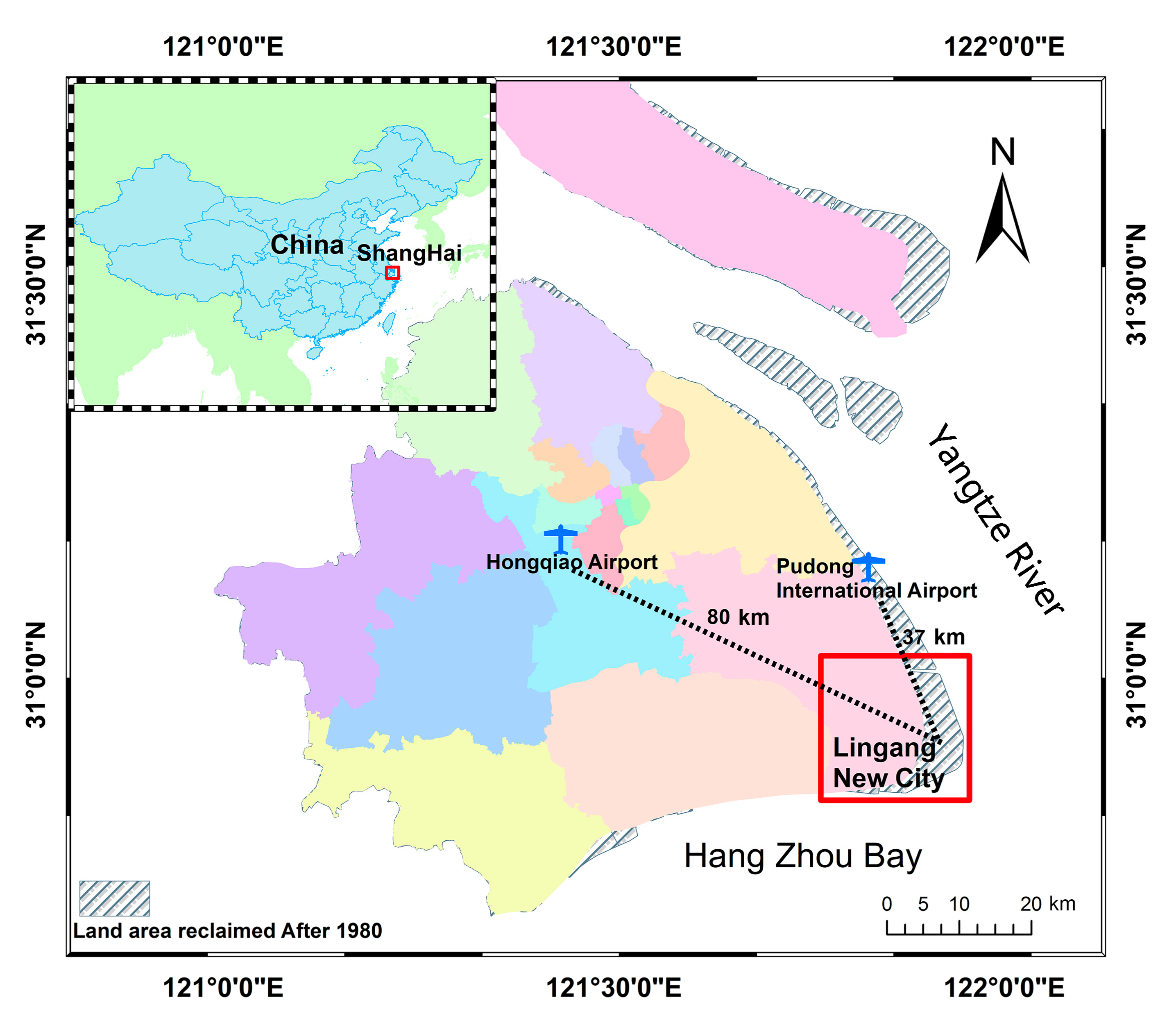
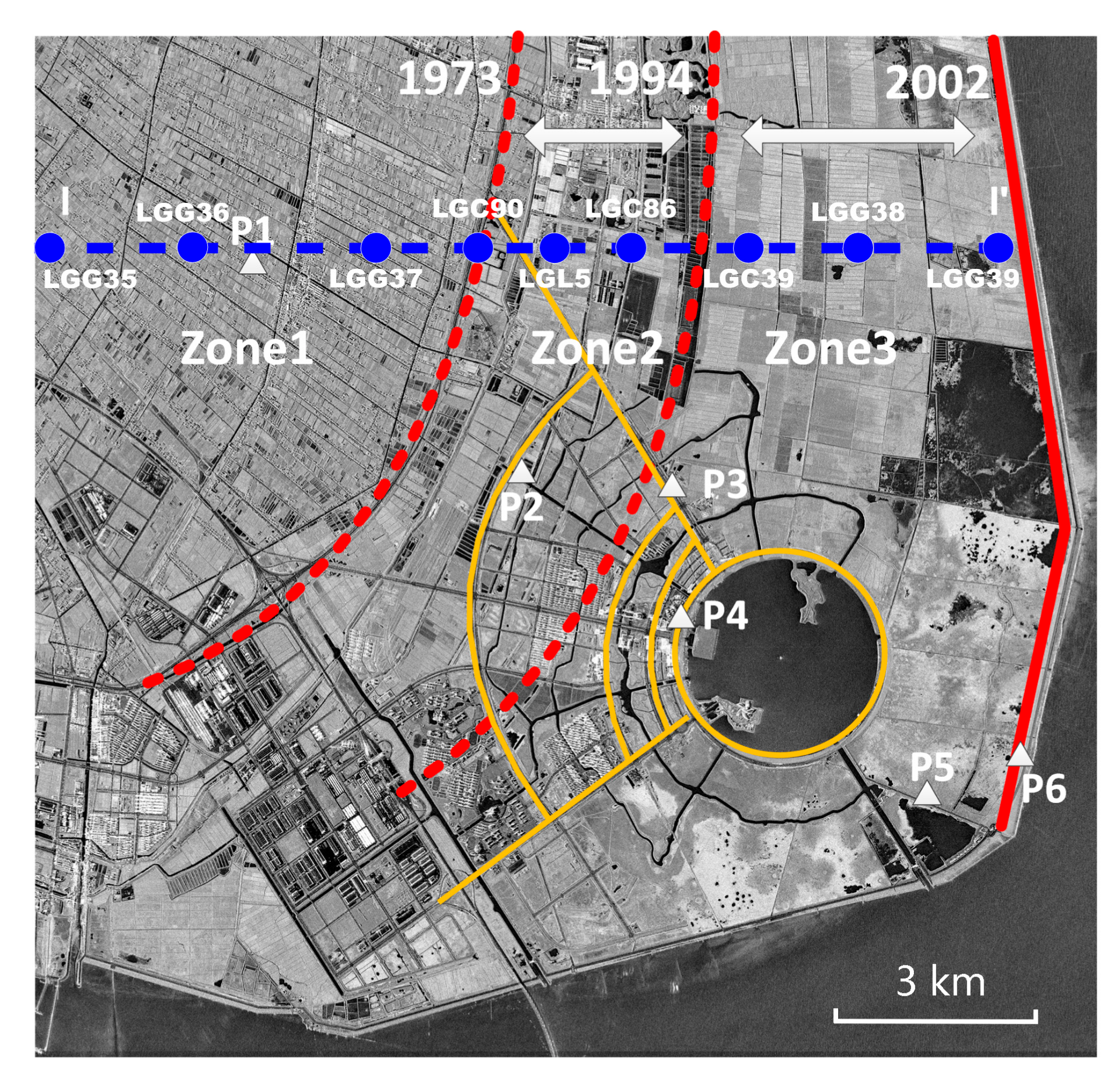
2. Study Area

The study area of Lingang New City (LNC) is geographically located at the south-eastern corner of Shanghai and close to the intersection of Yangtze River and Hangzhou Bay (approximately longitudes from 121.75°E to 122°E and latitudes from 30.84°N to 31.05°N). The LNC is 37 km from Pudong International Airport and 80 km from Hongqiao Airport, as shown in Figure 1. The total planned area of LNC is 311.6 km², including 133.3 km² (about 42 percent of total land area) created through reclamation projects [13]. The planning area of LNC is nearly one-third of Hong Kong’s land area (1104.43 km²) and around nine times as much as Macao’s land area (32.8 km²). Since 1973, five phases of the reclamation project have been carried out in the coastal areas of Shanghai, with five dams named by the year they were built: 1973, 1979, 1985, 1994 and the newest dam, built in 2002 [13]. Accordingly, the LNC area consists of various zones formed over different periods.

Three Landsat TM/ETM+ images acquired on 3 November 1999, 16 December 2003, and 6 May 2009 show the changes of this area in Figure 2. The coastal land shown in Figure 2a was formed before the new reclamation project. A new reclamation project was launched in 2003, and construction is scheduled to be completed in 2020 [13]. Figure 2b shows the LNC at the beginning of the project in 2003. The new land outside the coastline in 1999 was completed in 2009, and manmade features including a seawall, watercourse, and artificial lake can be easily identified in the 2009 image (see Figure 2c). The LNC was planned as a development area with multiple roles as an industrial area, shipping hub, and economic center.

LNC also contributes to the urban ecological system. According to the land use plan for the LNC in 2003 [13], less than 15% of the land is used for urban construction, around 55% of the land is agricultural, and around 30% is undeveloped. Therefore, LNC has wetlands and rich vegetation, which mitigates weather patterns and helps maintain ecological diversity.

3. Data and Methodology

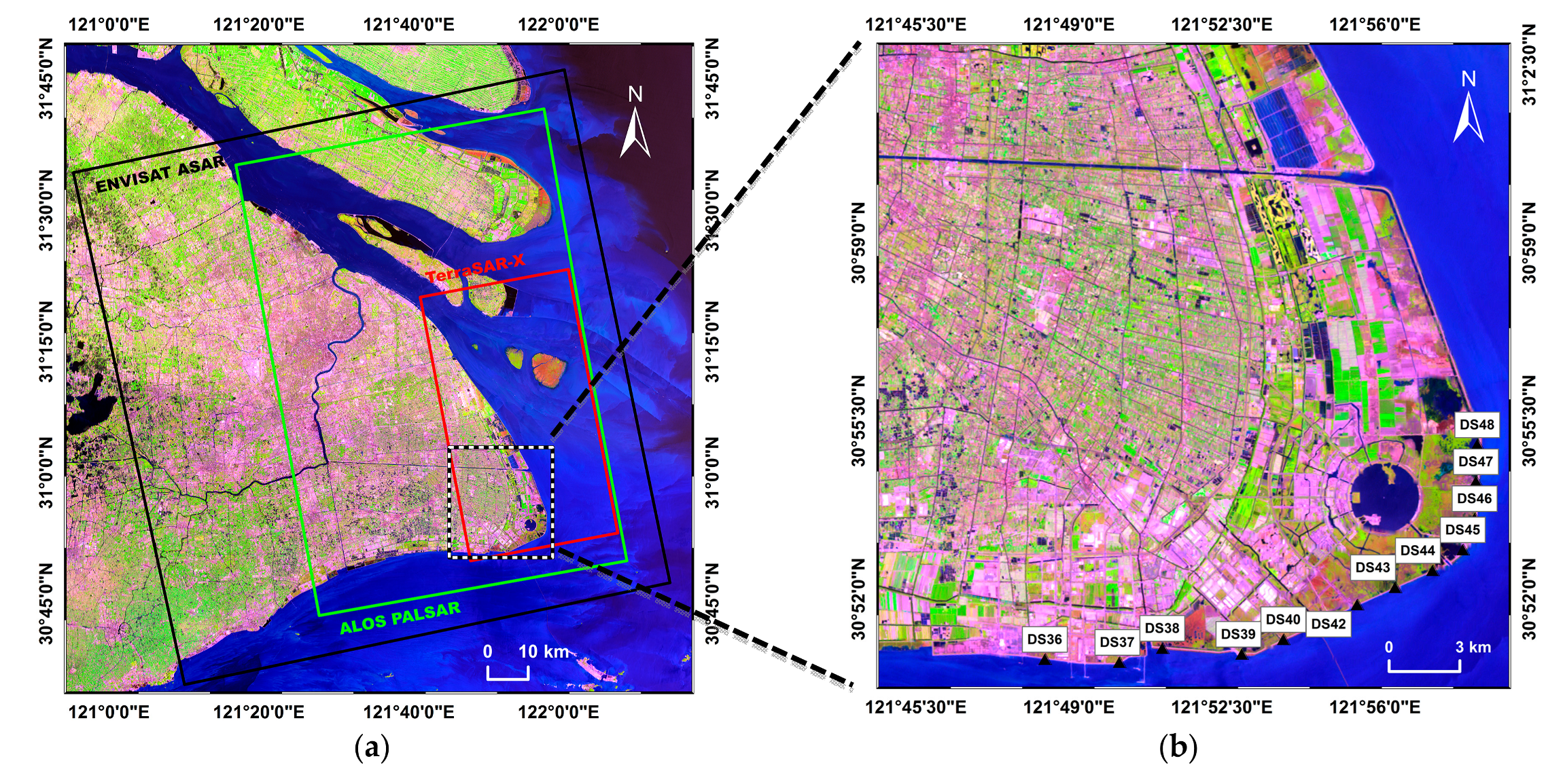
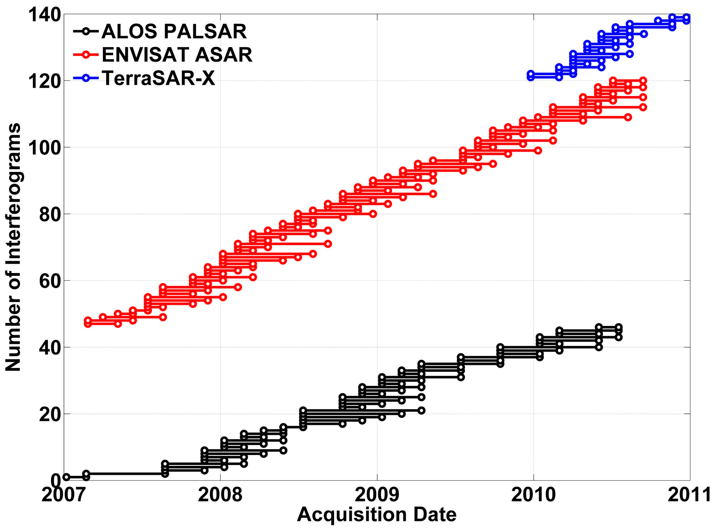
3.1. Data

We collected 66 satellite SAR images in three stacks, including 11 Stripmap (SM) mode images acquired by TerraSAR-X, 20 Fine Beam Single-polarization (FBS) and Fine Beam Dual-polarization (FBD) mode images acquired by ALOS PALSAR, and 35 Image Mode Single Look Complex (IMS) images obtained by ENVISAT ASAR. Figure 3a shows the coverage of the three data stacks, and

Table 1. Basic parameters of the three SAR data stacks.

Satellite/Parameter	TerraSAR-X	ALOS PALSAR	ENVISAT ASAR
Band (wavelength in cm)	X (3.1)	L (23.6)	C (5.6)
Acquisition dates	20091225~ 20101223	20070107~ 20100718	20070206~ 20100910
Number of images	11	20	35
Acquisition mode	SM	FBS&FBD	IMS
Pass direction	Ascending	Ascending	Ascending
Incident angle (°)	26.5	36.8	22.1
Heading (°)	349.24	347.21	346.80
Spatial coverage of full scene (range in km × azimuth in km)	30 × 50	70 × 56	100 × 100
Slant range spacing (m)	0.9	4.7 (FBS)/9.4(FBD)	7.8
Azimuth spacing (m)	2.0	3.1	4.0
Nominal critical baseline (m)	4000	9800	930
Track and frame	T5F167	T441F610	T497F603–621

summarizes the detailed parameters of these datasets. They are not fully overlapped in time. The three data stacks are obtained by the ascending mode, which cannot extract the east-west and vertical (up-down) components of deformations by a combination of three ascending and descending stacks. However, data stacks with slightly different imaging geometry provide a chance to cross-check against estimated results to reveal the deformation behavior in LNC. Moreover, previous results of LNC are based on C-band ENVISAT ASAR [9,10] from February 2007 to May 2010 and X-band COSMO-SkyMed [10] from December 2013 to March 2016. Here, we attached more attention to the results from X-band TerraSAR-X and especially L-band ALOS PALSAR.

The SAR data are paired to form interferograms with high coherence following small baseline rules. The maximum perpendicular baselines and temporal baselines were set to 300 m and 120 days for TerraSAR-X, 400 m; 210 days for Envisat ASAR; and 2800 m and 300 days for ALOS PALSAR. In total, 139 pairs were selected to form interferograms, including 19 from TerraSAR-X, 46 from ALOS PALSAR, and 74 from ENVISAT ASAR data stacks. The temporal distribution of all the interferograms is illustrated in Figure 4. The distribution maps of perpendicular baselines and temporal baselines of the three stacks are given as the supplementary material.

Another dataset used in this study is the in-situ leveling measurements. There are thirteen leveling benchmarks, distributed along the seawall in the LNC area, as shown in the Figure 3b. Two leveling measurement campaigns were carried out at all these 13 benchmarks on 9th January 2009 and 9th January 2010. The leveling data was acquired by the Shanghai Institute of Geological Survey (SIGS) following the specification of second-order leveling (±2 mm), and was processed with rigorous adjustment based on the theory of least squares estimation. The reference of leveling measurements is Chinese national height datum 1985. The height differences between two campaigns (one year interval) of 13 benchmarks were converted to the yearly velocities so that they could be used for validating InSAR results.

3.2. The SBAS-InSAR Technique

In this study, the SBAS-InSAR method [5,14] was employed to derive subsidence measurements in the LNC from the three satellite SAR data stacks. The steps in time series SAR data processing include differential interferograms generation, coherent point selection, network formation, phase unwrapping, and temporal-spatial filtering.

Differential interferograms are generated by separately subtracting the flat earth and topographic phase components from the original interferograms of the three data stacks. The phase observation at pixel x in the ith differential interferogram gives:

$${\psi }_{\mathrm{int},x,i}=W\left\{{\varphi }_{def,x,i}+{\varphi }_{atm,x,i}+\Delta {\varphi }_{\theta ,x,i}+\Delta {\varphi }_{orb,x,i}+{\varphi }_{n,x,i}\right\}$$

(1)

where $\mathrm{W}$ is the wrapping operator that truncates phase into the interval [−π, π] by modulo 2π, and ${\varphi }_{def,x,i}$ is the phase component corresponding to the target movement along the satellite line-of-sight (LOS) direction. The value ${\varphi }_{atm,x,i}$ is the phase signal induced by the difference in atmospheric path delay between two observations, $\Delta {\varphi }_{\theta ,x,i}$ is the residual phase of look angle error, $\Delta {\varphi }_{orb,x,i}$ is the phase of residual inaccuracy orbit, and ${\varphi }_{n,x,i}$ is the noise term.

CPs that maintain stable and strong backscattering signals over long time series observations were extracted from each data stack for differential interferometric phase analysis. In the LNC, there are a lot of vegetation-covered areas and built structures; thus, the phase noise is used as the indicator for CPs selection. It can identify reliable CPs in vegetated areas and areas with built structures. Phase noise ${\gamma }_x$ is defined as StaMPS [14]:

$${\gamma }_x=\frac{1}{N}\left|{\displaystyle \sum _{i=1}^N\exp \left\{j\left({\psi }_{\mathrm{int},x,i}-{\tilde{\psi }}_{\mathrm{int},x,i}-\Delta {\widehat{\varphi }}_{\theta ,x,i}^{nc}\right)\right\}}\right|$$

(2)

where N is the number of images, ${\tilde{\psi }}_{\mathrm{int},x,i}$ is the wrapped estimated of the spatially correlated parts of ${\psi }_{\mathrm{int},x,i}$, and $\Delta {\varphi }_{\theta ,x,i}^{nc}$ is the uncorrelated spatial component of $\Delta {\varphi }_{\theta ,x,i}$. Supposing that ${\varphi }_{def,x,i}$, ${\varphi }_{atm,x,i}$, and $\Delta {\varphi }_{orb,x,i}^{nc}$ are spatially correlated over a certain distance, and $\Delta {\varphi }_{\theta ,x,i}$ and ${\varphi }_{n,x,i}$ are uncorrelated over the same distance, then the uncorrelated spatial components of ${\varphi }_{def,x,i}$, ${\varphi }_{atm,x,i}$, and $\Delta {\varphi }_{orb,x,i}$ are small and are ignored. The phase noise of each pixel can be estimated by ${\gamma }_x$. Then, the CP candidates exceeding the noise threshold (in this case, we used 0.2π) are eliminated. Afterwards, for each stack, a triangulated irregular network (TIN) was built over the final CPs to establish the spatial network for phase unwrapping. Phase observations of the final group of CPs are unwrapped in both spatial and temporal dimensions to retrieve the deformation rates, as well as time series displacements. The detailed estimation algorithm of SBAS can be found in [5,14].

3.3. Vertical Displacement Estimation

Displacements by SBAS are given with respect to a reference pixel P, and relative to one reference acquisition time T. To compare results from different stacks, the three results must refer to a common pixel at the same reference time. A reference pixel is a common, stable pixel appearing in all three sets of results. In this work, the reference point is in the west corner of the Shanghai Ocean University, located in the stable area as identified in the Shanghai geological environment bulletin based on ground measurements including the leveling measurements [15,16]. A reference time is a common date of the three data stacks. However, three satellites have different revisiting intervals (11 days for TerraSAR-X, 35 days for ENVISAT ASAR, 46 days for ALOS PALSAR) and TerraSAR-X data covers only from 2009 to 2010, hence there are no data acquired on the same date. A compromise method is selecting acquisition dates adjacent to each other to achieve a common reference time. According to the acquisition date of SAR data, we have chosen 11-July-2010 for TerraSAR-X, 18-July-2010 for ALOS PALSAR, and 5-July-2010 for ENVISAT ASAR. Thus, the three sets of results refer to a generic pixel and the same reference date, the displacements of pixel P in T is zero, and all measurements are relative to this spatial-temporal reference point.

Furthermore, InSAR-derived displacements by SBAS are in LOS that must be converted to geographic space. Displacement in the LOS direction is a projection of the real deformation in east- west, north-south, and up-down directions. As SAR satellites are in a near-polar orbit with an angle between the flight direction and the north direction close to 10 degrees, InSAR observations have limited sensitivity to north-south displacement. Moreover, previous research indicated negligible west-east deformation in LNC [9,10]. Hence, we convert all the LOS measurements into a vertical direction according to incidence angles:

$$d_{\mathrm{v}}=\frac{d_{LOS}}{\cos \theta }$$

(3)

where $d_{\mathrm{v}}$ is the vertical deformation, $d_{\mathrm{LOS}}$ represents the displacements in the LOS direction, and $\theta$ is the incidence angle. Polynomial model fitting then estimates the subsidence rates with the extracted vertical deformation. For deformation decomposition, the optimal solution is combing the ascending and descending orbit for extracting deformation components in the east-west, north-south, and up-down directions. However, we do not have a descending data stack for this area during the same observation period. Another possibility is that we can compare the results from data stacks with slightly different imaging geometry to validate our assumption that vertical deformation is dominant. Such conversion also enables the validation of results against in-situ leveling measurements.

3.4. Results Validation

We evaluate the accuracy of InSAR-derived deformation measurements in two ways: an inner-precision check by consistency analysis among results and validation with independent ground measurements.

To perform consistency analysis among the results from the three SAR data stacks, we selected CPs with high coherence identified within the LNC area for comparative analyses. The threshold of coherence was set as 0.8 for initial candidate CP selection. In a given cross-stack CP pair (a, b), i.e., a and b are CPs chosen from two data stacks of A and B individually. If b is the nearest neighbor CP from B in object space for a, and vice versa, then, a and b will be identified as a common CP subject, if the Euclidean distance between them is less than 50 m. For each pair of data stacks, a linear fitting model of the mean deformation rate derived from one stack with respect to one derived from the other is established by least square estimation for the group of common CPs. The determination coefficient R², mean absolute difference, and standard deviation of absolute differences of CP pairs indicate the consistency of the results.

The absolute accuracy of deformation measurements derived from the three SAR data stacks is evaluated with respect to independent ground measurements. The leveling measurements are obtained at the benchmarks along the seawall in LNC following the specifications for second-order leveling (±2 mm) and were processed with rigorous adjustment based on the theory of least squares estimation. Indeed, two epochs of leveling measurements for 13 benchmarks in LNC are insufficient for evaluating all the InSAR results for multi epochs. However, these measurements do provide a reference independent of SAR satellite observations. Moreover, the locations of benchmarks are along the seawall, whose stability must be continuously monitored.

In consideration of the spatial and temporal mismatch between InSAR results and leveling measurements, two preprocessing steps are taken to enable the absolute accuracy assessment.

First, since there are only two phases of leveling measurements in January 2009 and January 2010, it is preferable to use InSAR-derived mean deformation rates over the same period for comparison. For ASAR and PALSAR data stacks, the appropriate subsets of derived time series deformations that are temporally closest to the leveling measurements are used to estimate the desired mean deformation rates. However, for the TerraSAR-X data stack, such a selection is not possible because there is almost no overlap in time between X-band observations and leveling measurements. Therefore, the deformation rates derived from the full X-band data stack are used in the comparison by assuming there is a linear deformation. Thus, the deformation rates of 2009 and 2010 are consistent.

Second, it is impossible to make direct one-to-one comparisons between CPs and leveling benchmarks because they are not located at exactly the same geographic position. As an alternative, a more practical average-to-one approach [17] is adopted to make the comparison. To be specific, for each leveling benchmark b_i, all CPs with a distance to b_i that is less than a predefined threshold T_d are chosen to form a group. Then, the arithmetic average of mean deformation rates at all CPs within this group is calculated as a representative to be used in comparison against the annual mean deformation rate measured by leveling. In this study, the value of distance threshold T_d was empirically set at 100 m. The mean values of differences and the corresponding standard deviations of InSAR results and leveling measurements are the indicators of absolute precision.

4. Results

4.1. Subsidence Rate Map

Using the method described in Section 3, we obtained the subsidence rates at selected CPs within the LNC from the three data stacks, as shown in Figure 5. Negative values of deformation rates indicate subsidence, while positive values represent uplift motions. In general, moderate (between −20 and −5 mm/y) to strong (<−20 mm/y) subsidence was observed in the newly reclaimed land close to the coastline. In contrast, most areas in the western part of the LNC appeared quite stable (between −5 and 5 mm/y), while gentle uplifts (between 5 and 10 mm/y) were clustered in the middle zone.

Similar spatial variability also exists over the newly reclaimed land, with subsidence in the northern part being more serious than in the southern part. According to a construction order [13], we divided the study area into three zones, i.e., zone1 formed before 1973, zone 2 formed between 1973 and 1994, and zone 3 formed after 2002. Locations of the three zones are illustrated in Figure 6. The southern part in zone 3 is the center of the LNC, and over the past decade, has developed more rapidly than the northern part in zone 3 (see Figure 2). Many factories, office blocks, residential buildings, and public infrastructures have been built in the southern part. Consequently, most CPs in the southern part were identified from new buildings and roads constructed on relatively stable piled foundations. Therefore, subsidence in the southern part is significantly slower than in the northern part, where there is subsiding soil. The deformation rates derived from the three different stacks show similar inhomogeneous spatial patterns as described. Furthermore, the distributions of selected CPs are not uniform. The CP density in the offshore area is lower than that in the inland area. Such a non-uniform spatial pattern can be largely attributed to the different stages of consolidation in the reclaimed zones. The relationship between observed deformation and reclamation projects is discussed in Section 5.3.

SBAS analyses were implemented on CPs that maintained coherence over time; the number and density of CPs will primarily determine the spatial sampling frequency. In general, a higher density of CPs is more likely to afford details of single objects. In this study, the total number and mean density (unit: CPs/km²) of CP points detected in the LNC area are 48872 and 128 for TerraSAR-X, 60683 and 112 for PALSAR, and 53783 and 70 for ASAR.

The highest mean density of CPs was detected in the urban area by the X-band TerraSAR-X data stack, followed by L-band and C-band data stacks. Two factors are involved. First, TerraSAR-X data has a higher spatial resolution than ASAR and PALSAR data, with which more details of ground features can be observed and thus more CPs can be detected at the same target. Second, the high density of detected CPs may benefit from the relatively short observation period, as well as from the frequent TerraSAR-X acquisitions.

As shown in Figure 5, in the southern part of zone 3 where a residential urban area is located, all the three data stacks manifested similar capabilities of detecting numerous CPs with stable and strong backscattering signals. Nevertheless, the north part of zone 3, marked as A in Figure 5, in the rural area covered with vegetation, an entirely different pattern appeared. Very few CPs were detected from X- and C-band data stacks, whereas quite a few CPs were still identified from the L-band data stack. Such an advantage of using L-band data can be attributed to its capabilities of deeper penetration into vegetation and better resistance to temporal de-correlation related to the longer wavelength.

To examine more closely the performance of the PALSAR data stack, we focused on two marked areas, A and B, shown in Figure 5. In the marked area A, few points are identified by X-band (Figure 5a) and C-band (Figure 5c) data stacks, and most of the points were detected along the road. However, the result of the L-band (Figure 5b) data stack provides detailed deformation rates except for the two small ponds in this area. In the marked area B, results based on X-band (Figure 5a) and C-band (Figure 5c) data stacks failed to detect the deformation in the marked area B because no CP was selected. The result of the L-band (Figure 5b) data stack shows there is a severe subsidence. A quantitative comparison among the three stacks and absolute precision validation will be elaborated in Section 5.1 and Section 5.2.

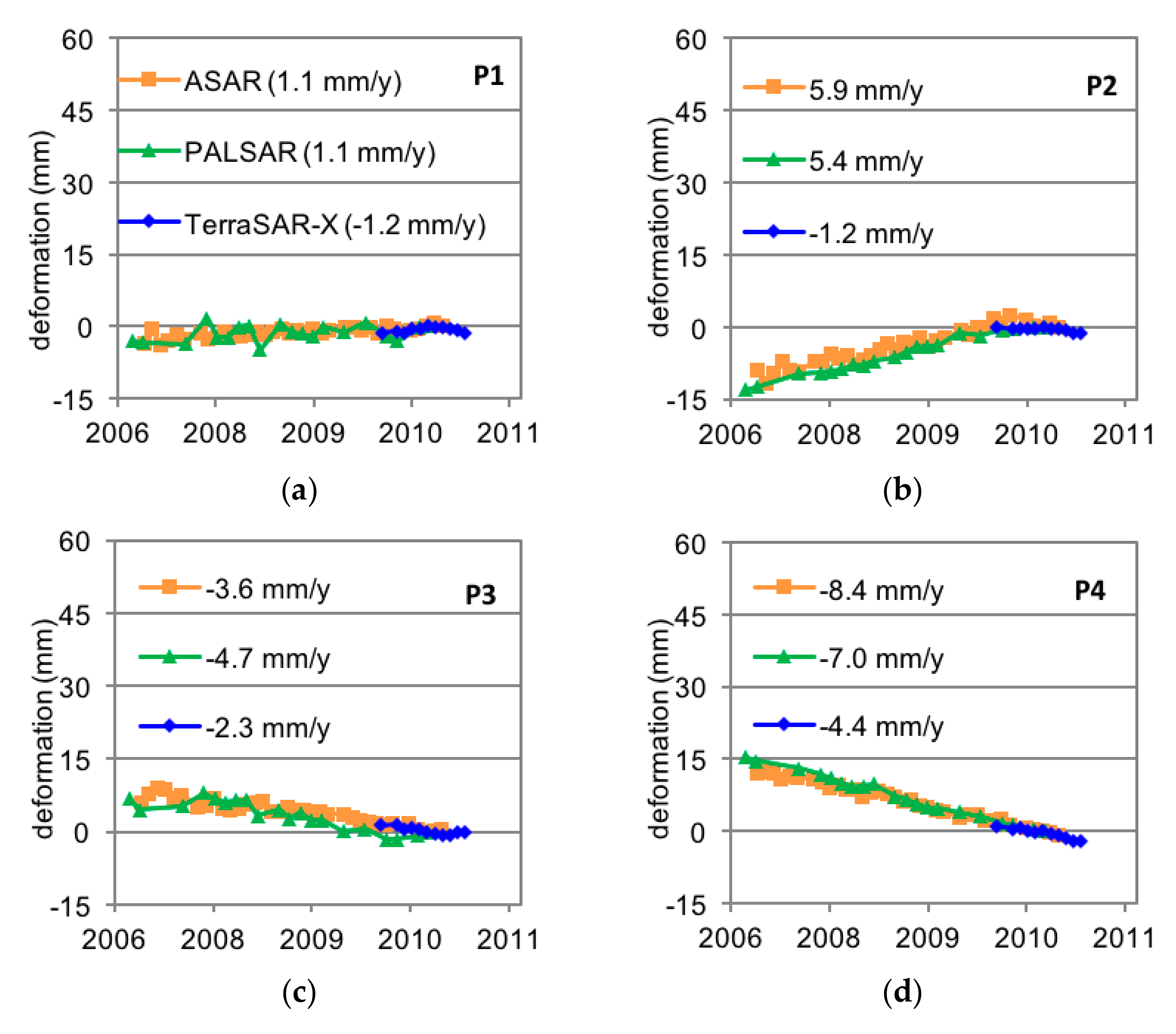
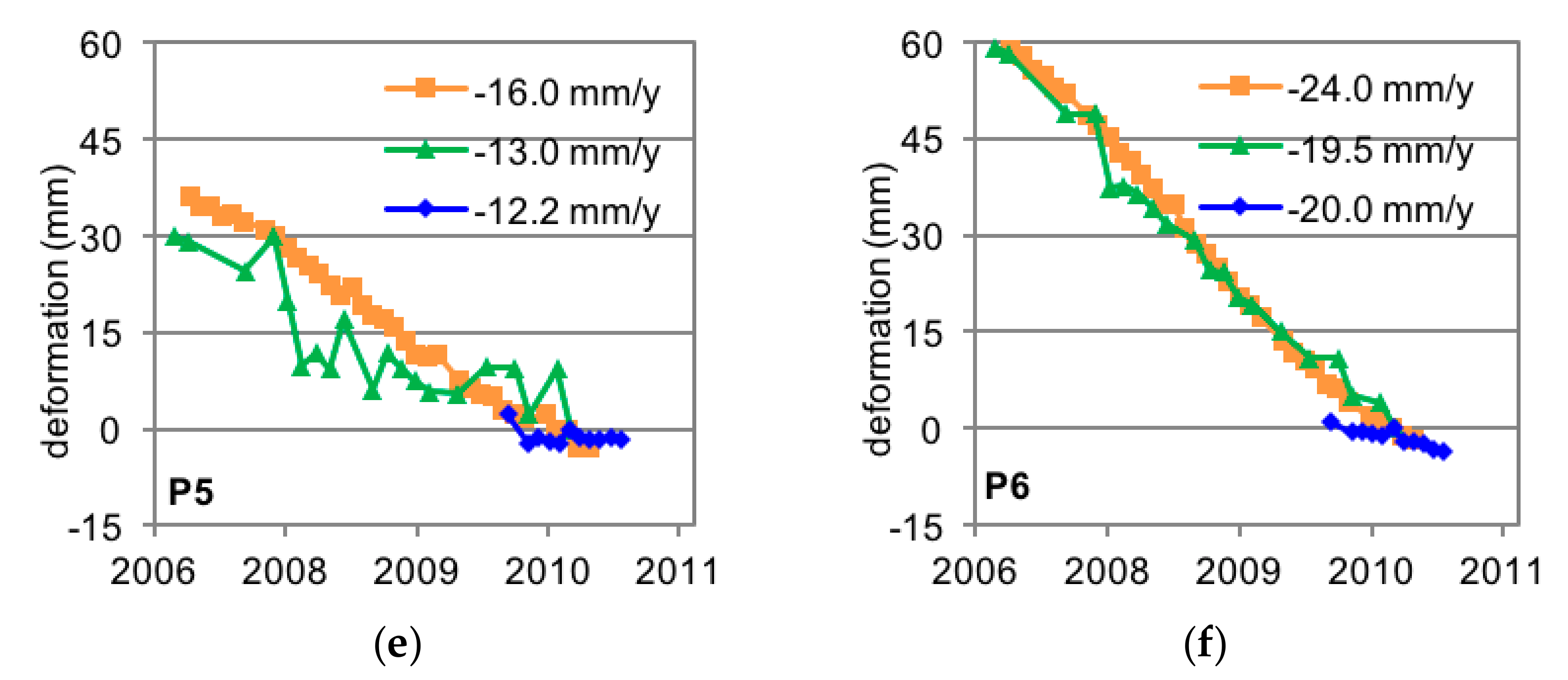
4.2. Time Series Deformation of Selected CPs

To evaluate the spatial distribution and temporal evolution of deformation, six CPs were selected in different zones: P1 in zone 1; P2 in zone 2; and P3, P4, P5, and P6 in zone 3. The locations of the selected CPs are shown in Figure 6. P1 is in the stable area shown in Figure 5, P2 is in the middle area with slight uplifts, and P3, P4, P5, and P6 are in the newly reclaimed land that is close to the coastline. There are three extra points selected in zone 3 because of the spatial variability of subsidence within this area, as denoted in Figure 5.

Figure 7 shows the time series deformation of six CPs: (a) P1, (b) P2, (c) P3, (d) P4, (e) P5, and (f) P6 from ASAR, PALSAR, and TerraSAR-X data stacks. Time series deformation measured at CPs reflects the detailed changes of the CPs in the observation period relative to the measurement in the selected reference time. The data acquisition times of ASAR and PALSAR were from 2007 to 2010 and TerraSAR data was collected from 2009 to 2010. Thus, the overlapping time in July 2010 was chosen as the reference time. As indicated in Figure 7, P1 is quite stable as it underwent only a slight fluctuation around zero from 2007 to 2010; whereas P2 shows a trend of gentle uplift before September 2009 and afterward zero-centered subtle fluctuation. The other four CPs (P3, P4, P5, and P6) experienced linear subsidence at various velocities from 2007 to 2010, with the fastest and slowest subsidence appearing at P6, located on the seawall, and P3 at a more inland location. However, such a subsidence trend at all four points slowed down in 2009 and then transformed into a relatively mild pattern of subsidence, which might indicate that the newly reclaimed land has entered the stage of long-term slow compression. In Section 5.3, Section 5.4 and Section 5.5 we will further discuss the spatial distribution and temporal evolution of deformation in LNC in joint analyses of reclamation activities, local geological data, and the soil mechanisms.

5. Discussion

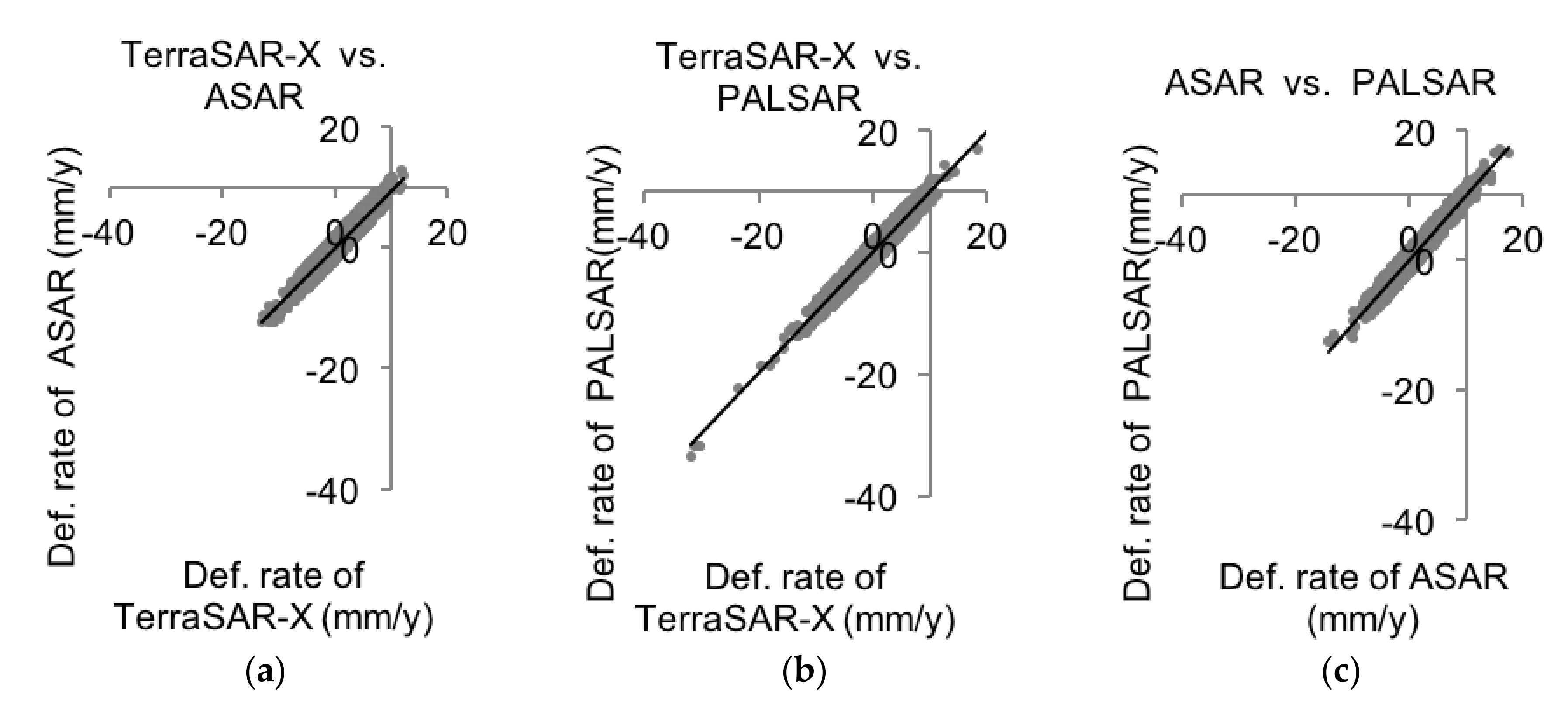
5.1. Consistency Analysis among InSAR-Derived Results

Consistency analysis among the results from the three SAR data stacks was carried out. We estimated a linear fitting model of the mean deformation rate derived from one stack with respect to a model derived from the other two stacks by least square estimation using the entire group of common CPs. Scatter plots for these models are shown in Figure 8, with the corresponding mathematical expressions and related statistics summarized in

Table 2. Results of cross validation among the three SAR data stacks.

Satellite/Parameter	TerraSAR-X vs. PALSAR	TerraSAR-X vs. ASAR	ASAR vs. PALSAR
Number of common CPs	1863	2987	1866
Mathematical expression of linear model	Y = 0.9x	Y = 0.9x	Y = 0.9x
Coefficient of determination R2	0.9	0.9	0.9
Mean absolute difference (mm/y)	0.9	0.7	0.2
Standard deviation of absolute differences (mm/y)	3.6	3.4	3.9

. When making comparisons between TerraSAR-X and the other two data stacks, the time interval used for mean deformation rate estimation was set as from late 2009 to middle 2010.

From Figure 8 and Table 2, it can be seen that the three coefficients of determination are around 0.9, which indicates that highly similar spatial patterns in the mean deformation rate were detected by the three SAR data stacks. The mean and standard deviation of absolute differences for the three pairs were less than 1 mm/y and 4 mm/y, respectively, showing an overall good agreement among the deformation measurements derived from the three SAR data stacks. Several CPs in areas with relatively fast subsidence (mean deformation rate < −20 mm/y) were identified by both X-band and L-band data stacks simultaneously. These were excluded from the groups of identical CPs for linear fitting between the C-band result and that of X-band or L-band. This phenomenon might be caused by the weaker capability of the ASAR data stack to detect fast deformation, as compared to the TerraSAR-X and PALSAR observations used in this study.

This comparison was based on the extracted vertical displacement. Thus, the good agreement among these InSAR-derived results also validates our claim that the east-west component of displacements, with respect to the vertical deformation, is negligible.

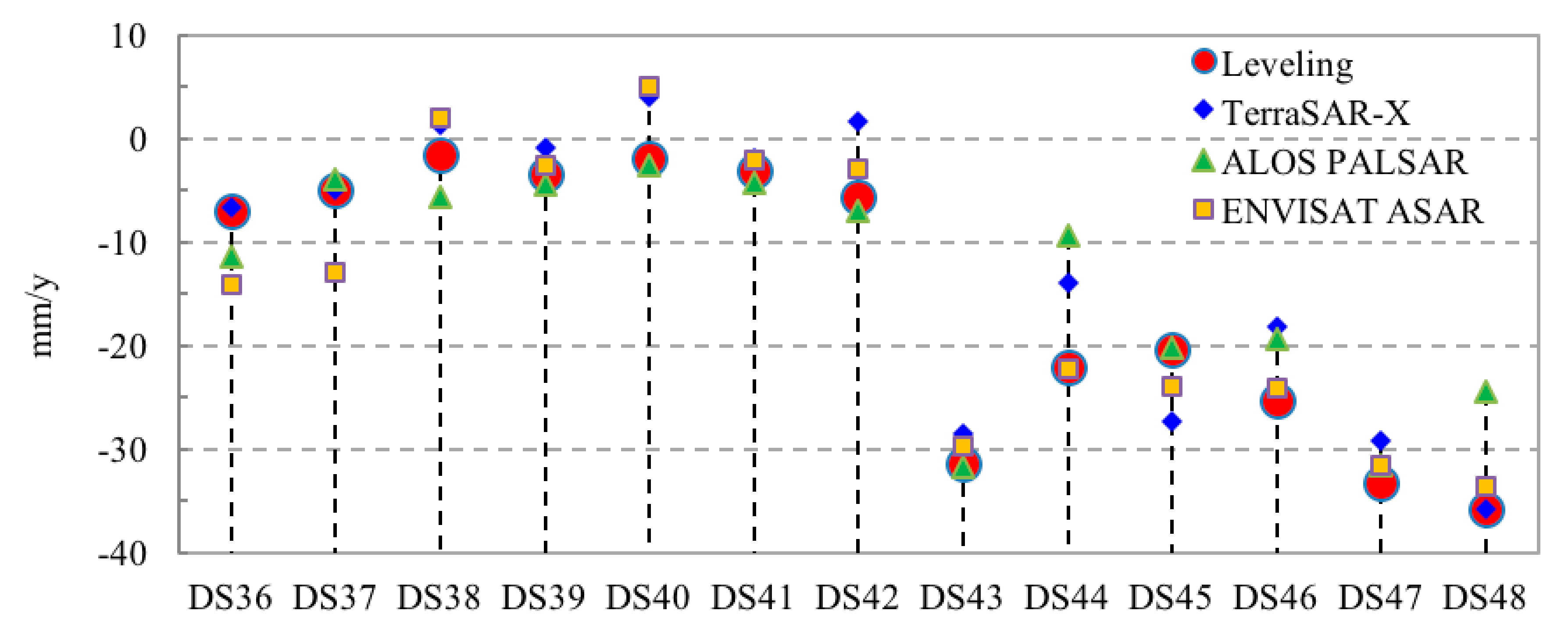
5.2. Validation with Leveling

The absolute accuracy of deformation measurements derived from the three SAR data stacks was evaluated with respect to independent ground measurements. The results of the absolute accuracy assessment at 13 leveling benchmarks are plotted in Figure 9. According to the leveling measurements, large subsidence (<−20 mm/y) occurred along the eastern section of the seawall in the LNC (from DS43 to DS48), while in the southern section (from DS36 to DS42), only slight to moderate subsidence was detected. Such a spatial variability was also revealed by InSAR results from the three data stacks, showing overall good agreement with leveling measurements. The arithmetic mean values of differences are 2.7, 1.5, and 0.2 (mm/y) for TerraSAR-X, PALSAR, and ASAR, respectively, and the corresponding standard deviations are 4.7, 5.3, and 4 (mm/y). Therefore, we can conclude that all the three data stacks achieved millimeter-level accuracy. The relatively larger differences for X-band data are likely due to temporal mismatch, while the best performance by C-band data might be attributed to its more frequent observations during the period.

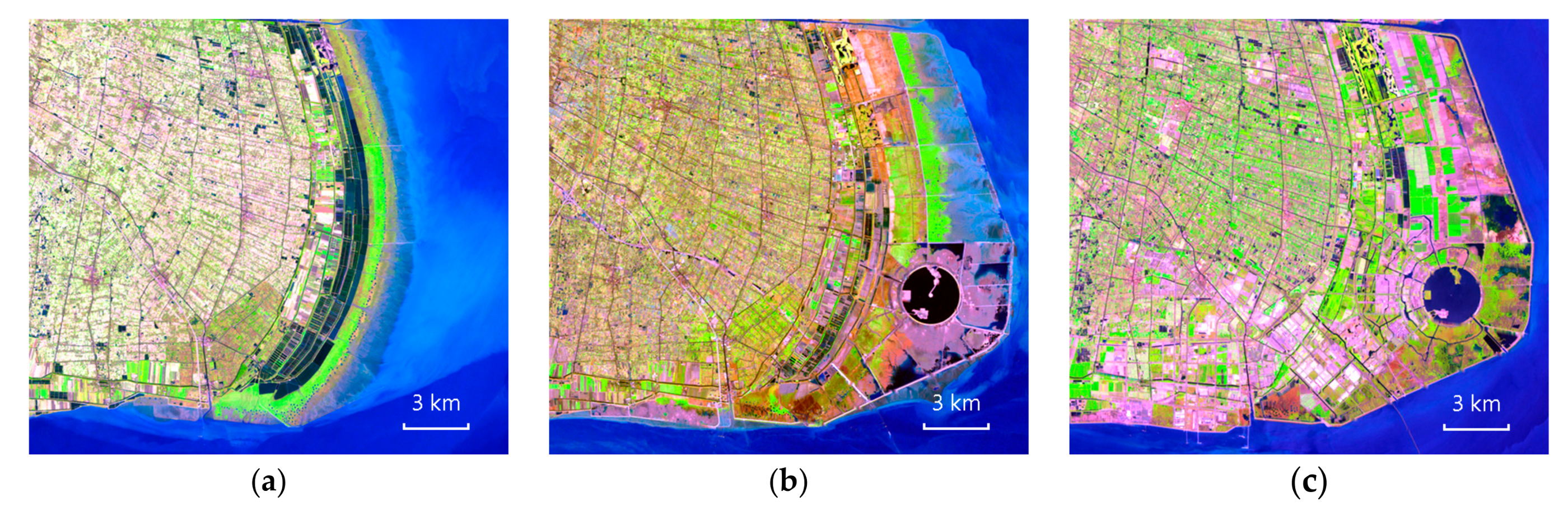
5.3. Analysis of Observed Subsidence and Reclamation Evolution

We also explored the relationship between InSAR-observed ground subsidence and reclamation evolution. As shown in Figure 6, we divided the study area into three zones considering that the construction order for LNC Zone 1 was established before 1973, in zone 2 the construction order was set between 1973 and 1994, and in zone 3, it was formulated from 2002.

As shown in Figure 5, many CPs were detected in zone 1 and zone 2. Since the reclamation projects in these two zones have been completed for more than a decade, most CPs in these two zones exhibited relatively good stability (between −5 and 5 mm/y). Compared to the stable older zones, an overwhelming subsiding tendency with relatively high deformation rates (<−10 mm/y) was detected in zone 3, reclaimed after 2002. The fillings used for reclamation in the LNC are characterized by a high void ratio, large compressibility, and low strength. This zone was still experiencing a consolidation procedure, consistent with the established Terzaghi theory which assumes that the primary consolidation could last for a few years [18]. This situation was also verified by the time series deformation of CPs in the three zones. As indicated in Figure 7, P1 in zone 1 was quite stable from 2007 to 2010, whereas P2 in zone 2 shows a slight uplift. P3, P4, P5, and P6 illustrate the spatial variability of subsidence within zone 3.

To quantitatively evaluate the corresponding relationships between the reclamation phases and observed subsidence, the mean deformation rates over the three zones derived from the three SAR data stacks were calculated and summarized in

Table 3. Deformation rates of the three zones (unit: mm/y).

Mean Deformation Rate (Standard Deviation)		SAR SENSOR
		TerraSAR-X	ALOS PALSAR	ENVISAT ASAR
zone	1	−0.5 (3.9)	−0.8 (9.9)	1.3 (5.0)
	2	2.4 (4.3)	4.8 (11.9)	6.1 (6.4)
	3	−7.9 (9.1)	−12.1 (19.5)	−11.3 (20.3)

. The mean deformation rates of points of the three zones describe the main trends within each zone, and the standard deviations of zones illustrate variation in the velocities of deformation in each zone and probable error. Therefore, the standard deviation increase from zone 1 to zone 3 indicates that the spatial variation was the largest in zone 3. Moreover, the standard deviation of ALOS PALSAR is larger than the other two, which indicates that the phase noise in the PALSAR data is larger. All the three mean values across zone 1 are around ±1 mm/y, which again confirms its relative stability. In the meantime, the moderate positive value and large negative value of the mean deformation rate for zone 2 and zone 3 indicate, individually, a gentle uplift and rapid subsidence during the study period. Therefore, it is evident that these three zones were in different consolidation periods, corresponding to the reclamation activities at different times.

According to the spatial distribution and temporal evolution of deformation, we infer three stages of surface changes in LNC after the reclamation project. For newly reclaimed areas such as zone 3, the consolidation will last for a few years. This primary consolidation is the first stage of changes after reclamation. Then, it enters the second stage, which is a slight rebound after long-term compression. The second stage elaborates the changes in the area, which build for a while during a reclamation project; zone 2 has been established for more than ten years. Finally, subsidence will stay at a steady level after long-term changes. Zone 1 exhibits this stability, which has developed over a period of more than 30 years.

5.4. Geological Features

In this section, we further analyze the observed settlements with the geological features in the LNC. The different components and lithology of the underlying soil are important factors influencing the subsidence of LNC [15,16,19,20]. Soft soil in LNC can be divided into seven engineering geological layers (①–⑦) based on their geological ages, soil behaviors, and physical and mechanical properties.

Table 4. The division of engineering geologic layers in LNC.

Geological Age		Layer Number and Lithology	Deposit Type	Distribution Area	Foundation Conditions
Holocene $Q_h$	$Q_h^3$	①1 Dredger fill	Artificial	Whole area	Not as foundation
		①3 Dredger fill	Reclaiming project	The eastern and southern part of LNC	Prone to liquefaction
		②1 Silty clay	Supralittoral	The western part of LNC	Compression layer
		②3 Sandy silt	Mesolittoral	Whole area	Prone to quicksand
	$Q_h^2$	④ Muddy clay	Littoral-shallow sea	Whole area	Compression layer
	$Q_h^1$	⑤1-1 Clay	Supralittoral	Whole area	Compression layer
		⑤1-2 Silty clay	Supralittoral	Widely distributed	Compression layer
		⑤2 Sandy silt	Swampy	Sporadically distributed	Poor holding layer for foundation
		⑤3 Silty clay with silt	Swampy	Paleo-rivers area
Late Pleistocene $Q_{p3}$	$Q_{p3}^2$	⑤4 Silty clay	Swampy	Paleo-rivers area
		⑥ Clay	Plain-lake	Mainly in LNC area	Good holding layer for construction piles
		⑦1 Silt with silty	Estuary Marina	Whole area
		⑦2 Silt with silty	Estuary Marina	Whole area

gives detailed information about each layer.

The dredger fill layer ①₃ is mainly distributed in the eastern and southern part of the LNC. Dredger fill is a kind of unconsolidated soil with a high water content, large void ratio, and high compressibility. Therefore, land subsidence is prone to occur during the initial period of a reclamation project. Moreover, the thickness of dredger fill is different as the LNC was built in a multi-phase reclamation project. In the areas built before 1994 (zone 1 and zone 2), the thickness of the dredger fill is around 2–3 m. The fill is in normal consolidation phase. The fill in zone 3, the area reclaimed after 1994, is unconsolidated with an increasing thickness of 3–6 m from the inland to the coast. Therefore, most of the subsidence occurred in the eastern and southern part of LNC.

Silty clay ②₁ is mainly distributed in the west and north part of the LNC at a depth of 0.5–1.5 m with a thickness of 0.5–2 m. A silty clay layer can be used as the natural foundation of small construction due to its low water content, compressibility, and void ratio. This layer shows a relatively stable engineering characteristic compared to ①₃. This agrees with our results that the western and northern parts of the LNC are more stable than the southern and eastern parts of the LNC. Sandy silt ②₃ is distributed across the whole area, which is prone to quicksand. The thickness of the shallow sand layer is around 6 to 14 m and increases from the northwestern to southeast. Therefore, the different consolidation stages of ①₃, and the distribution of ①₃ and ②₁, as well as the thickness changing of shallow sand layer ②₃ together, contribute to the spatial variability of subsidence in the LNC.

The soft soil layer ④ and clay layer ⑤ were distributed in the whole LNC area. Muddy clay ④ is a soft soil typical of Shanghai with a high water content and compressibility. It is easily deformed during construction. Clay layers ⑤ are not a good foundation for buildings except the secondary hard soil layer⑤₄. The clay layer ⑤₁ and ⑤₂ are the compression layers of the larger construction projects. Attention must be paid to the compaction of the soft soil layer ④ and clay layer ⑤ in civil engineering. The widespread hard soil layer ⑥ and sand bed ⑦ originated in the late Pleistocene and are a suitable foundation layer for structures, having nothing to do with the displacements in the LNC.

Figure 10 shows a geological section map of a profile line I-I’ as indicated in Figure 6, from 45 m below ground to several meters above ground. Gray represents layer ①₁, faint yellow represents silty clay ②₁ and ⑤₄, cyan represents ①₃, orange with dark dots represents ②₃, blue represents ④, orange with oblique line represents ⑤_1-1, faint yellow represents ⑤_1-2, green represents ⑥, beige with dotted line represents ⑦₁, and yellow represents ⑦₂. Nine drill holes of the profile line are in different zones: LGG35, LGG36, and LGG37 in zone 1; LGC90, LGL5, and LGC86 in zone 2; and LGC39, LGG38, and LGG39 in zone 3. Hence, the changes in the geological section of nine drill holes describe the underlying soil features of the area formed in different periods.

As illustrated in Figure 10, the geological section of nine drill holes is roughly the same. Specifically, the thickness of each layer of LGG35, LGG36, and LGG37 is relatively the same, which indicates a stable geological condition; while the thickness of holes in zone 2 and zone 3 increases relative to the holes in zone 1. Furthermore, the thickness changes are mainly in the compression layers: topsoil of loose and newly deposited soil layers ①₃, Sandy silt ②₃, soft soil layers ④ and clay layer ⑤, and especially ⑤₁. The consolidation of underlying soil causes the subsidence in the LNC. As described, the different consolidation stages of dredger fill①₃, the distribution of the dredger fill layer ①₃, relatively stable silty clay layer ②₁, the thickness changing of the shallow sand layer ②₃, soft soil layer ④ and the clay layer ⑤ together, contribute to the spatial variation of subsidence in the LNC.

5.5. Compression Mechanism of Hydraulic Fill

In this section, we discuss the observed deformation with the compression mechanism of hydraulic fill. The hydraulic fill in the LNC is mainly the soft alluvial soil [19,20]; therefore, the three stages are explained by the compression mechanism of soft soil. There are two critical compressibility indexes for soft soil: the compression index and resilience index. Previous studies [18,21,22] give the relationship between soil matric suction and the compression index/resilience index of the Shanghai area, which can be used for analyzing the spatial distribution and temporal evolution of deformation in the LNC. Figure 11 gives the effects of soil matrix suction on the compression index and resilience index. The compression index declines with soil matric suction growth, slowly arriving at a plateau. While the resilience index first decreases with an increase in matric suction, it goes up as the suction continuously increases.

We explain the temporal evolution of subsidence in the LNC with the compression mechanism of hydraulic fill. We argue that the external forces in a newly reclaimed area are constant, but at the beginning, the consolidation pressure increases as the matric suction increases. Thus, the void ratio decreases gradually, which shows the continuous subsidence in the area during the first stage. Meanwhile, the compression index first decreases and then reaches stability gradually, with an increase in matric suction. However, the rebound index first decreases with an increase of matric suction. When the matric suction is higher than a certain amount, it increases with the rise of matric suction. The slight rebound in the area after a period of reclamation project reflects the growth in the rebound index. Stability occurs when the rebound index and compression index reach equilibrium. Thus, the third stage reflects the balance of rebound index and compression index, and this might take the time to reach, in this case, more than 30 years.

6. Conclusions

In this paper, time series InSAR analyses are carried out with X-, C-, and L-band SAR data stacks to retrieve the subsidence velocity and time series of surface deformation at the LNC in the Shanghai metropolis. A cross-comparison of the results of the three data stacks and validation with leveling measurements demonstrates the performance of these data in land subsidence monitoring. Furthermore, an evaluation of spatial distribution and temporal evolution of deformation in the LNC was conducted by joint analyses of deformation measurements, historical reclamation activities, local geological data, and soil mechanisms. The main conclusions are summarized as follows:

(1)

Cross-comparisons of the three results suggest that PALSAR works at a longer wavelength, which makes it much less affected by undesired temporal decorrelation and has advantages when mapping newly reclaimed areas. Cross-validation shows a good agreement among mean deformation rates measured at CPs shared by the three data stacks, with the coefficients of determination around 0.9 and the standard deviations of inter-stack differences less than 4 mm/y. The good agreement validates our argument of the negligibility of the east-west component of displacement with respect to the vertical deformation. Validations with leveling data collected at benchmarks along the seawall indicate that all the three data stacks achieved millimeter-level accuracy. The mean values of differences were 2.7, 1.5, and 0.2 (mm/y) for TerraSAR-X, PALSAR, and ASAR, respectively, and the corresponding standard deviations were 4.7, 5.3, and 4 (mm/y).

(2)

The results from the three data stacks show a similar spatial variability of land subsidence across the LNC area. Specifically, overall good stability was observed within the area built before 1973 in the west of LNC, while moderate to large subsidence occurred within the coastal area built after 2002 in the east, and gentle uplift existed within the area built in 1994. A quantitative evaluation of observed subsidence with the historical reclamation activities indicates the spatial variability of land subsidence in the LNC, related to multi-phase reclamation and urban construction projects.

(3)

The analysis of local geological data indicates that the consolidation of underlying soil causes the subsidence in LNC. Specifically, the different consolidation stages of dredger fill①₃, the distribution of dredger fill layer ①₃, relatively stable silty clay layer ②₁, the thickness changing of the shallow sand layer ②₃, soft soil layer ④ and the clay layer ⑤ together, contribute to the spatial variation of subsidence in the LNC.

(4)

Three stages of evolution in the reclaimed area were derived from the observed subsidence in the LNC, verified by the soft soil mechanisms. The first stage is the primary consolidation stage, which can last for a few years. The second stage is the slight rebound stage after long-term compression. The final stage is a state of stable equilibrium.

References

- McLeod, E.; Poulter, B.; Hinkel, J.; Reyes, E.; Salm, R. Sea-level rise impact models and environmental conservation: A review of models and their applications. Ocean Coast Manag. 2010, 53, 507–517. [Google Scholar] [CrossRef]
- Haas, J.; Ban, Y. Urban growth and environmental impacts in Jing-Jin-Ji, the Yangtze, River Delta and the Pearl River Delta. Int. J. Appl. Earth Obs. Geoinf. 2014, 30, 42–55. [Google Scholar] [CrossRef]
- Crosetto, M.; Monserrat, O.; Cuevas-González, M.; Devanthéry, N.; Crippa, B. Persistent Scatterer Interferometry: A review. ISPRS.J. Photogramm. 2016, 115, 78–89. [Google Scholar] [CrossRef]
- Ferretti, A.; Prati, C.; Rocca, F. Permanent scatterers in SAR interferometry. IEEE Trans. Geosci. Remote Sens. 2001, 39, 8–20. [Google Scholar] [CrossRef]
- Berardino, P.; Fornaro, G.; Lanari, R.; Sansosti, E. A new algorithm for surface deformation monitoring based on small baseline differential SAR interferograms. IEEE Trans. Geosci. Remote Sens. 2002, 40, 2375–2383. [Google Scholar] [CrossRef]
- Van Leijen, F.J. Persistent Scatterer Interferometry Based on Geodetic Estimation Theory. 2014. Available online: https://www.ncgeo.nl/index.php?option=com_k2&view=item&id=2669:persistent-scatterer-interferometry-based-on-geodetic-estimation-theory&Itemid=350&lang=en (accessed on 22 February 2018).
- Casu, F.; Manzo, M.; Lanari, R. A quantitative assessment of the SBAS algorithm performance for surface deformation retrieval from DInSAR data. Remote Sens. Environ. 2006, 102, 195–210. [Google Scholar] [CrossRef]
- Raucoules, D.; Bourgine, B.; de Michele, M.; Le Cozannet, G.; Closset, L.; Bremmer, C.; Veldkamp, H.; Tragheim, D.; Bateson, L.; Crosetto, M.; et al. Validation and intercomparison of Persistent Scatterers Interferometry: PSIC4 project results. J. Appl. Geophys. 2009, 68, 335–347. [Google Scholar] [CrossRef]
- Zhao, Q.; Pepe, A.; Gao, W.; Lu, Z.; Bonano, M.; He, M.L.; Wang, J.; Tang, X. A DInSAR Investigation of the ground settlement time evolution of ocean-reclaimed lands in Shanghai. IEEE J. Sel. Top. Appl. 2015, 8, 1763–1781. [Google Scholar] [CrossRef]
- Pepe, A.; Bonano, M.; Zhao, Q.; Yang, T.; Wang, H. The use of C-/X-Band Time-Gapped SAR data and geotechnical models for the study of Shanghai’s ocean-reclaimed lands through the SBAS-DInSAR technique. Remote Sens. 2016, 8, 911. [Google Scholar] [CrossRef]
- Jiang, L.; Lin, H. Integrated analysis of SAR interferometric and geological data for investigating long-term reclamation settlement of Chek Lap Kok Airport, Hong Kong. Eng. Geol. 2010, 110, 77–92. [Google Scholar] [CrossRef]
- Jiang, L.; Lin, H.; Cheng, S. Monitoring and assessing reclamation settlement in coastal areas with advanced InSAR techniques: Macao city (China) case study. Int. J. Remote Sens. 2011, 32, 3565–3588. [Google Scholar] [CrossRef]
- Shanghai Urban Planning and Design Research Institute. The Master Plan of Lingang New City. Shanghai Urban Plan. Rev. 2009, 4, 11–26. (In Chinese) [Google Scholar]
- Hooper, A. A multi-temporal InSAR method incorporating both persistent scatterer and small baseline approaches. Geophys. Res. Lett. 2008, 35. [Google Scholar] [CrossRef]
- Shanghai Municipal Bureau of Planning, and Land Resources. Shanghai Geological Environmental Bulletin (2009). Available online: http://www.shgtj.gov.cn/dzkc/dzhjbg/201007/t20100728_407604.html (accessed on 22 February 2018). (In Chinese)
- Shanghai Municipal Bureau of Planning, and Land Resources. Shanghai Geological Environmental Bulletin (2010). Available online: http://www.shgtj.gov.cn/dzkc/dzhjbg/201307/t20130718_600136.html (accessed on 22 February 2018). (In Chinese)
- Fuhrmann, T.; Caro Cuenca, M.; Knöpfler, A.; Van Leijen, F.J.; Mayer, M.; Westerhaus, M.; Hanssen, R.F.; Heck, B. Estimation of small surface displacements in the Upper Rhine Graben area from a combined analysis of PS-InSAR, levelling and GNSS data. Geophys. J. Int. 2015, 203, 614–631. [Google Scholar] [CrossRef]
- Terzaghi, K.; Peck, R.B.; Mesri, G. Soil Mechanics in Engineering Practice; John Wiley & Sons: Hoboken, NJ, USA, 1996; pp. 1–592. [Google Scholar]
- Shen, S. Geological environmental character of Lin-Gang new city and its influences to the construction. J. Shanghai Geol. 2008, 105, 24–28. (In Chinese) [Google Scholar]
- Shi, Y.; Yan, X.; Zhou, N. Land subsidence induced by recent alluvia deposits in Yangtze River delta area, a case study of Shanghai Lingang New City. J. Eng. Geol. 2007, 15, 391–402. (In Chinese) [Google Scholar]
- Xie, N.; Sun, J. The rheological properties of soft soils in Shanghai. J. Tongji Univ. Nat. Sci. 1996, 24, 233–237. (In Chinese) [Google Scholar]
- Ye, W.; Zhu, Y.; Chen, B.; Ye, B. Compressibility of Shanghai unsaturated soft soil. J. Tongji Univ. Nat. Sci. 2011, 39, 1458–1462. (In Chinese) [Google Scholar]