Analysis of Permafrost Region Coherence Variation in the Qinghai–Tibet Plateau with a High-Resolution TerraSAR-X Image


1
Faculty of Information Engineering, China University of Geosciences, 388 Lumo Road, Wuhan 430074, China
2
The Key Laboratory of Digital Earth Science, Institute of Remote Sensing and Digital Earth, Chinese Academy of Sciences, Beijing 100094, China
*
Author to whom correspondence should be addressed.
Remote Sens. 2018, 10(2), 298; https://doi.org/10.3390/rs10020298
Submission received: 1 November 2017
/
Revised: 2 February 2018
/
Accepted: 13 February 2018
/
Published: 15 February 2018
(This article belongs to the Special Issue Remote Sensing of Dynamic Permafrost Regions)
Abstract
:The Qinghai–Tibet Plateau (QTP) is heavily affected by climate change and has been undergoing serious permafrost degradation due to global warming. Synthetic aperture radar interferometry (InSAR) has been a significant tool for mapping surface features or measuring physical parameters, such as soil moisture, active layer thickness, that can be used for permafrost modelling. This study analyzed variations of coherence in the QTP area for the first time with high-resolution SAR images acquired from June 2014 to August 2016. The coherence variation of typical ground targets was obtained and analyzed. Because of the effects of active-layer (AL) freezing and thawing, coherence maps generated in the Beiluhe permafrost area exhibits seasonal variation. Furthermore, a temporal decorrelation model determined by a linear temporal-decorrelation component plus a seasonal periodic-decorrelation component and a constant component have been proposed. Most of the typical ground targets fit this temporal model. The results clearly indicate that railways and highways can hold high coherence properties over the long term in X-band images. By contrast, mountain slopes and barren areas cannot hold high coherence after one cycle of freezing and thawing. The possible factors (vegetation, soil moisture, soil freezing and thawing, and human activity) affecting InSAR coherence are discussed. This study shows that high-resolution time series of TerraSAR-X coherence can be useful for understanding QTP environments and for other applications.
1. Introduction
Permafrost is defined as soil or rock that remains at or below 0 °C for two or more consecutive years [1]. The Qinghai–Tibet Plateau (QTP) is the region with greatest permafrost in the world, and it affects its surrounding environment and climate directly through atmospheric and hydrological processes [2,3]. The top layer of the ground subject to annual thawing and freezing in areas underlain by permafrost is defined as the active layer (AL) [4]. Global warming influences the thawing and freezing processes of AL, and consequently its carbon storage [5]. In turn, the status of permafrost in Tibet is a sensitive indicator of global climate change. Long-term temperature measurements indicate that the lower altitudinal limit of permafrost has moved by 25 m in the north during the last 30 years [6,7]. Numerous studies have been conducted on permafrost degradation and its effect on infrastructure construction, especially since 2006 when the Qinghai–Tibet Railway (QTR) was completed [8,9,10,11]. The existence of the QTR has changed the thermal exchange between the ground surface and the atmosphere, and influenced the underlying permafrost environment, resulting in the increase of the ground temperature and acceleration of the process of permafrost degradation [8]. Some thaw hazards have occurred along the embankment of the QTR. Therefore, it is important to further study the permafrost environment in the QTP.
Conventional methods for studying a permafrost environment include soil-moisture retrieving, deformation monitoring, active-layer thickness estimation and other hydrological factors based on point-based field measurement [10,11,12,13]. However, these methods are time-consuming and cannot provide deformation maps with high spatial-sampling density. Due to its advantages of high resolution and large coverage, synthetic aperture radar interferometry (InSAR) has been used for plateau deformation monitoring and soil-moisture retrieving; the technique has yielded good results [14,15,16]. The space scale of InSAR observation ranges from one to several hundred kilometers. The accuracy of InSAR measurements relies heavily on the presence of pixels that hold stable properties during the observation of interest. However, the accuracy of conventional InSAR is limited by variable atmosphere signal delay, and temporal and geometric decorrelation. In order to overcome those limitations, several time-series InSAR techniques, such as persistent scatterer interferometry (PSI) [17,18] and the small baseline subset algorithm (SBAS) [19,20], have been proposed in the past decade. By analyzing a long time series of interferometry phases on stable objects such as buildings, rocks and roads, these techniques can obtain long-term ground movement with millimeter-level accuracy. Numerous studies have been conducted to monitor the stability of the permafrost area using time-series InSAR methods [14,15]. However, due to the global and seasonal temperature changes, the backscattering feature of the ground targets in the permafrost region change considerably during the freezing and thawing cycle, which contributes decorrelations and limits the application of InSAR in this region.
Coherence is an important parameter, which is a good indicator of the phase stability of scatterers. High coherence simplifies phase unwrapping and enhances the reliability of a derived digital elevation model (DEM) or displacement in InSAR methods [21]. A high coherence value means that the surface properties exhibit minimal changes over two observations, whereas a low coherence value indicates substantial surface variation during the timescale (temporal decorrelation). The magnitude of the complex coherence of an interferometric SAR pair can be used to qualify changes in image pixels. In recent years, seasonal coherence analysis has been performed in permafrost regions to detect the temporal change of the ground condition [22,23]. Wickramanayake et al. investigated all possible interferometric combinations of 34 RADARSAT-2 (C-band) images in order to evaluate coherence variability with respect to temporal baseline and master image data in Kiruna, northern Sweden [22]. Antonova et al. studied the spatial and temporal variability of radar backscatter and coherence over the Lena River Delta using 35 TerraSAR-X images [23]. Therefore, studying seasonal coherence variation can be useful for understanding permafrost environments and for other applications.
The objective of this paper is to investigate the potential of the high resolution X-band image for monitoring permafrost environment change in Beiluhe permafrost area. Seventeen TerraSAR-X Staring Spotlight (ST) mode images with HH polarization acquired from June 2014 to August 2016, covering the full range of thawing and freezing, were used in this study. Time-series coherence maps were obtained and the coherence seasonal variations of typical ground targets were analyzed. A temporal decorrelation model containing a long-term and a seasonal-term component has been proposed. The effects of possible environmental factors and human activity on the coherence change are discussed.
2. Study Area and Dataset
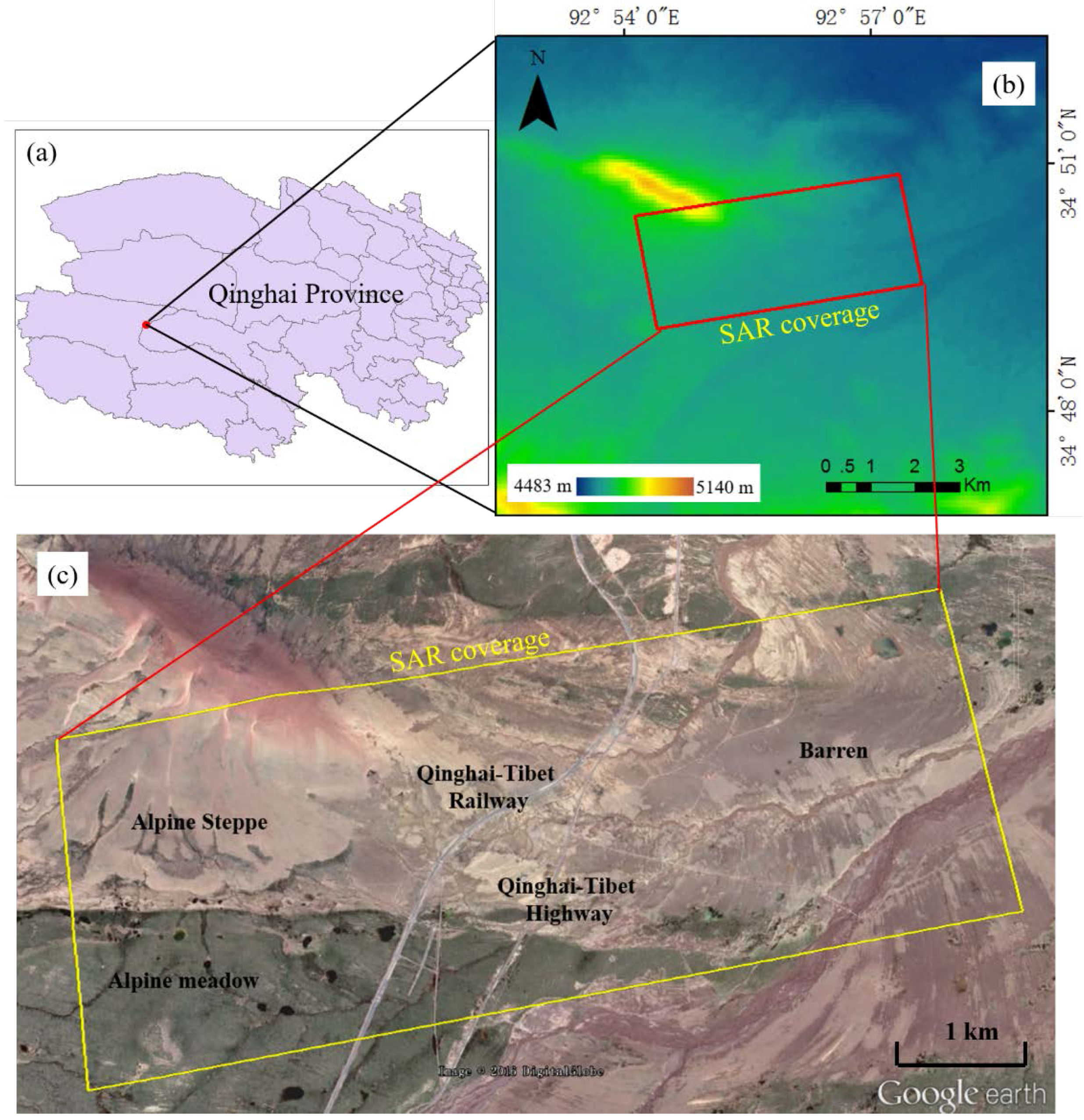
The test site is located in the south-west of Qinghai Province, China. The temperature changes greatly from the summer season to the winter season, with the maximum high and low air temperatures reaching approximately 23 °C and −38 °C, respectively. Figure 1a shows air temperature in the study area measured by the Beiluhe weather station. Due to the occurrence of such a broad temperature change, the permafrost environment is highly variable and vulnerable during a one-year cycle. The monthly precipitation from May 2014 to October 2015 was collected (see Figure 1b). The monthly precipitation ranges from 20 mm to 100 mm and most of the precipitation is concentrated in the summer season. The elevation of the study area ranges from 4483 m to 5140 m (see Figure 2b) It is a low-temperature permafrost region with continuous perennial permafrost and ice-rich active layers. The active layer thickness (ALT) ranges from 1.5 m to 3 m in our study area [2]. Due to the effect of the thawing and freezing, the maximum seasonal deformation reaches up to 10 cm [15].
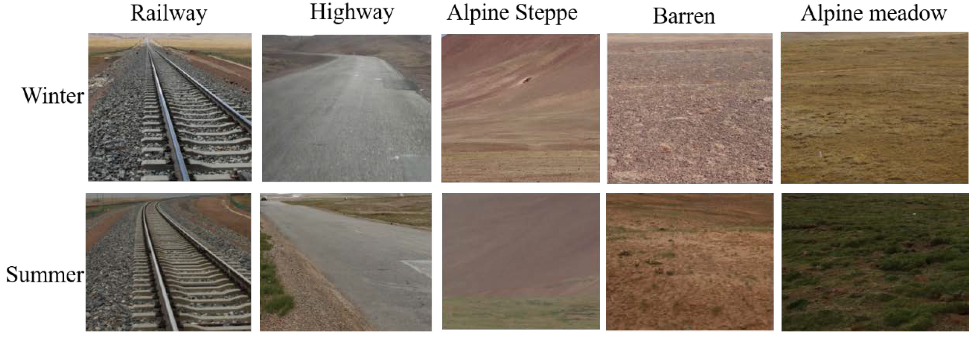
Based on a Google map (see Figure 2c), and the field photos of the study site, it is apparent that typical ground features in this study area contains 5 types: railway, highway, alpine steppe, barren, and alpine meadow, which are selected as the typical ground features for coherence analysis. Figure 3 shows field photos of typical ground targets in the winter and summer seasons. From Figure 3, we can observe that, except for the railway and highway, the surface environment of the other three types changes greatly from the winter to summer season, especially in alpine meadow areas. Several thermokarst lakes, are distributed in the region. Due to global warming, the areas of those thermokarst lakes are becoming larger. In this study, it is assumed that the thawing season begins on 15 April and the freezing season begins on 1 October [2]. In summer, due to the thawing of AL and the rainy weather, the soil’s water content begins to increase and the alpine meadow grows rapidly. The height of the vegetation is approximately 10 cm. In winter, all the alpine meadow and parse vegetation wither (see Figure 3). In the winter season, most of the study area is dry. In those areas, fallen snow may be readily blown away. But in the water regions, such as the thermokarst lakes and rivers, accumulated snow can be found.
To monitor the coherence variation of the study area, 17 TerraSAR-X ST mode ascending images acquired from June 2014 to August 2016 with an incidence angle of 23.5 degrees and ‘HH’ polarization are used (see Table 1). The coverage of the SAR image is about 2.8 × 7.5 km2 (shown in Figure 2b) The pixel spacings of the complex images in the range and azimuth direction are 0.454 m and 0.167 m, respectively. After all the radar images were co-registered, 136 interferograms were generated. Then, using the Shuttle Radar Topography Mission (SRTM) co-registered to the master image, differential interferograms were obtained.
3. Method
3.1. Coherence
For given two single-look complex (SLC) SAR images, interferometric coherence is defined as the magnitude of the complex cross-correlation coefficient, which can be calculated to identify the similarity between the two SAR images. Interferometric coherence is frequently used as a parameter to evaluate the phase stability of interferograms [24]. Moreover, interferometric coherence can also reflect change information of the surface ground targets across two time periods, which can be used as a classification parameter. The normalized coherence can be expressed as [25]:
where, r is the coherence value at pixel (x, y); S1, and S2 are the complex values of master SAR image and the slave SAR image at pixel location (x, y), respectively; and * represents the complex conjugation. The brackets indicate a local spatial averaging around the pixel (x, y). The r value is related with the window size. In this paper, the window size is 3 × 3 pixels. The absolute value of r, the interferometric coherence, ranges from zero (decorrelated signals) to one (fully correlated signals).
The coherence value is influenced by several factors, which can be expressed as a product of the respective decorrelation factors [26]:
where is the baseline decorrelation; is the temporal decorrelation; is the decorrelation related to thermal noise in the SAR system; and is the decorrelation related with volume scattering.
The influence of baseline decorrelation on coherence loss can be calculated using the formula [26]:
where B is the baseline; Sr is the range resolution; θ is the incidence angle; λ is the wavelength; and R is the slate range distance. For TerraSAR-X images used in this study, taking the large baseline in our dataset (500 m), incidence angle (23.5°), rbaseline is about 0.975, suggesting that the influence of the spatial baseline on coherence loss can be neglected. depends on systemic thermal noise, which can be ignored for a modern SAR System [27,28]. is not considered in this case because this study area is not in a high-penetration area such as forest [29]. Consequently, the contribution of those above decorrelation components is relatively small, and the effects of the temporal decorrelation are the factor.
3.2. Modelling of Temporal Decorrelation
Temporal decorrelation is caused by changing physical properties of the ground between two acquisitions. In [26], the temporal coherence was determined by an exponential temporal-decorrelation component plus a thermal-noise component. In most areas, this exponential temporal-decorrelation model is practical and has been used in several applications [30,31]. However, in a permafrost area, except for the long-term temporal decorrelation, the seasonal temporal decorrelation is serious due to the thawing and freezing effect of the AL. The evolution of the permafrost layer, active layer, soil moisture, climate, and hydrology jointly determining the ground physical characteristics and then the coherence. Ignoring the sudden or complete change that could be modeled, the ground surface-change processes in the permafrost area can be divided into two: a long-term process and a seasonal process. The long-term process is mainly affected by the climate warming and permafrost thawing-induced process. The seasonal process is more complex and drastic than that of the long-term process. The factors determining the seasonal process are related to the temperature. Most important is the freeze–thaw cycle of the active layer, which would change the form of soil and moisture content with the season, thus affecting the characteristics of surface roughness, liquid moisture content, and periodic deformation characterized by frost heave and thaw settlement, and thus lead to seasonal decorrelation of the radar wave [32].
Considering that, a temporal coherence model is determined by a linear temporal decorrelation component plus a seasonal periodic decorrelation component and a constant component, which can be expressed as:
where rmn is the coherence between the mth and nth SAR images; ∆t is the temporal baseline of the mth and nth SAR image (days); T is the duration of the thawing and freezing cycle; at this site, T = 365 days. a, b, and c are the variable parameters.
3.3. Time-Series Coherence Analysis
The first step of InSAR processing is co-registration. The first image of the images stack was selected as the master image, and the remaining SAR images were co-registered to the master image. In this paper, the correlation function method is used for the SAR image registration. In order to get the interferogram, the accuracy of the registration must be less than 1/8 pixel. A total of 136 raw interferograms were then produced by multiplying one image with the complex conjugate of the other images for all possible image-pair combinations. Then, the topographic phase and flat earth phase were removed from the raw interferograms by using the SRTM DEM. After that, adaptive Goldstein filtering was used to decrease the noise. Then the coherence value and interferometric phase can be calculated from the raw interferogram. A 3 × 3 moving window was applied for the coherence-magnitude calculation. In this study, inspired by the work of Wickramanayake et al. [22], the time-series coherence maps were arranged in two groups: the common master group (CMG) and the sequential master group (SMG). In general, arranging the coherence maps in two sets can be useful for the analysis of coherence seasonal variation. In the CMG, the image acquired in the winter season (2 December 2014) was selected as the common master image. Table 2 shows the details of the interferograms in CMG. In the SMG, interferometric coherence images have minimum temporal baselines. Table 3 shows the selected sequential interferograms.
4. Experimental Results
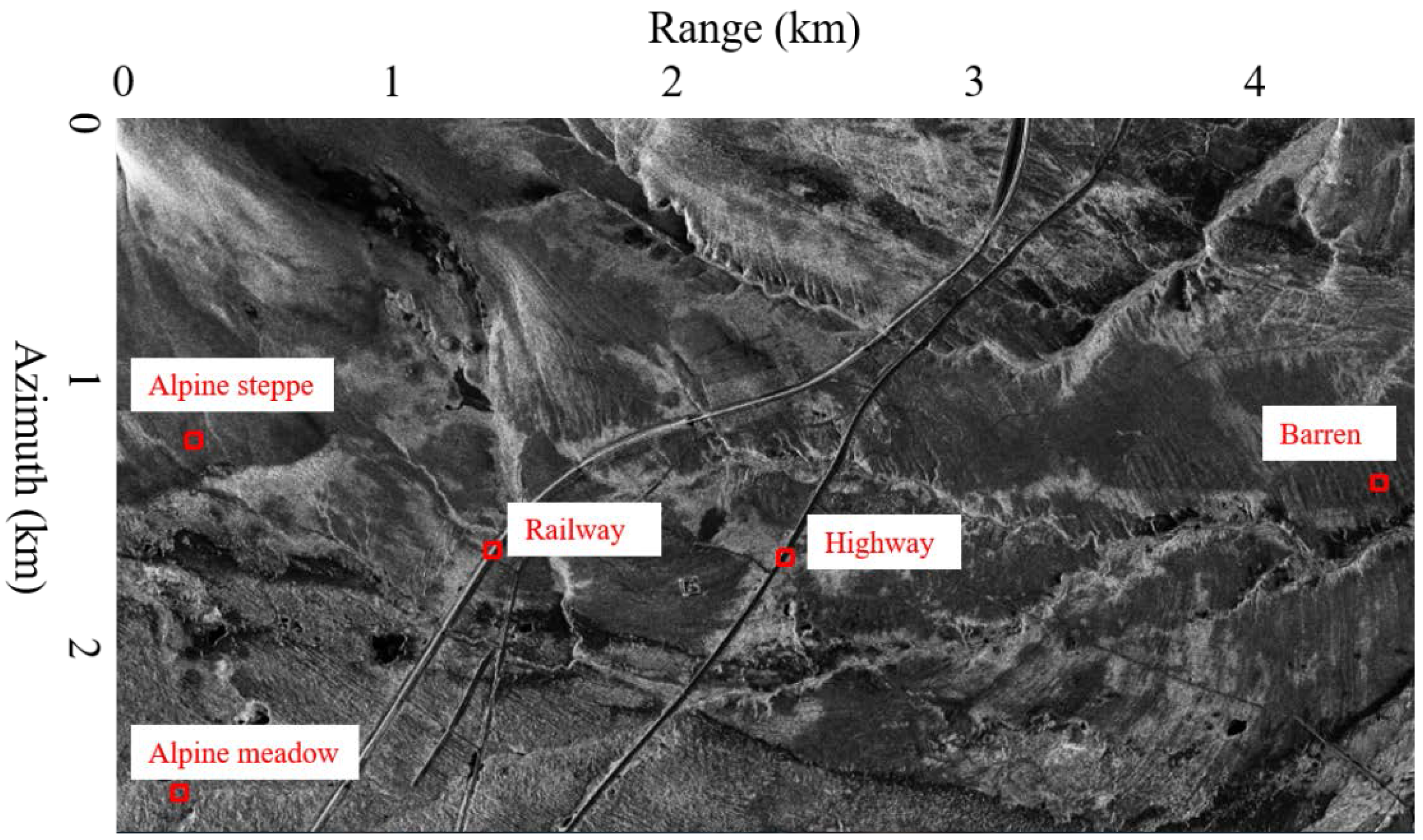
In our study area, the ground targets are a mix of natural, anthropogenic, and morphometric classes. In the SAR images, those targets are strong coherence objects (railway, highway), partial coherence objects (mountain slope, barren), and decorrelation objects (alpine meadow) [33]. The objective of this paper is to analyze the variable of the permafrost coherence. Considering that, five typical ground features are selected and the locations of the selected samples are shown in Figure 4. For each type of ground feature, we get the mean coherence value by averaging the samples with the window of 9 × 9.
4.1. Time-Series Interferometric Coherence
The spatial and temporal baselines for the CMG are shown in Figure 5. In the CMG, all the baselines are less than 500 m, and the baseline decorrelation can be neglected (as analyzed in Section 3.1). The consistent summer–winter and winter–winter combinations were contained and could be used for the seasonal analysis.
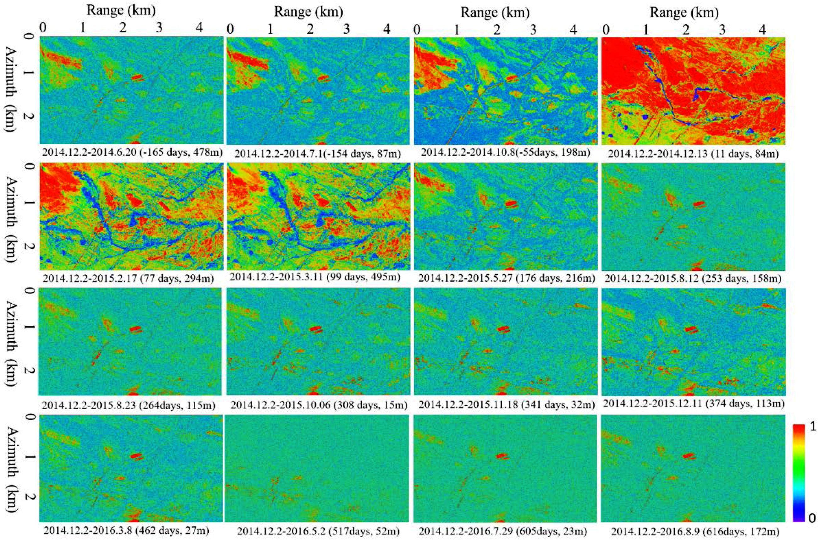
Figure 6 displays the time-series coherence maps of the study site for the CMG. The SAR image acquired on 2 December 2014 is the common master image. The coherence value is notably lower in summer season and higher in winter season. When the master image and slave image were acquired both in winter season, a higher-quality coherence map can be obtained because the surface environment of the permafrost changes little during the winter season. When the master image and slave image were acquired in difference seasons, the coherence map exhibits greater noise due to temporal decorrelation. In the winter season, the permafrost surface is in a dry condition and soil moisture is close to zero. During the summer season, the permafrost surface experiences a thawing condition and soil moisture increases; these conditions are suitable for alpine vegetation growth. It is the environmental difference between the winter and summer seasons that contributes to the serious decorrelation in coherence maps of summer–winter interferometric combinations.
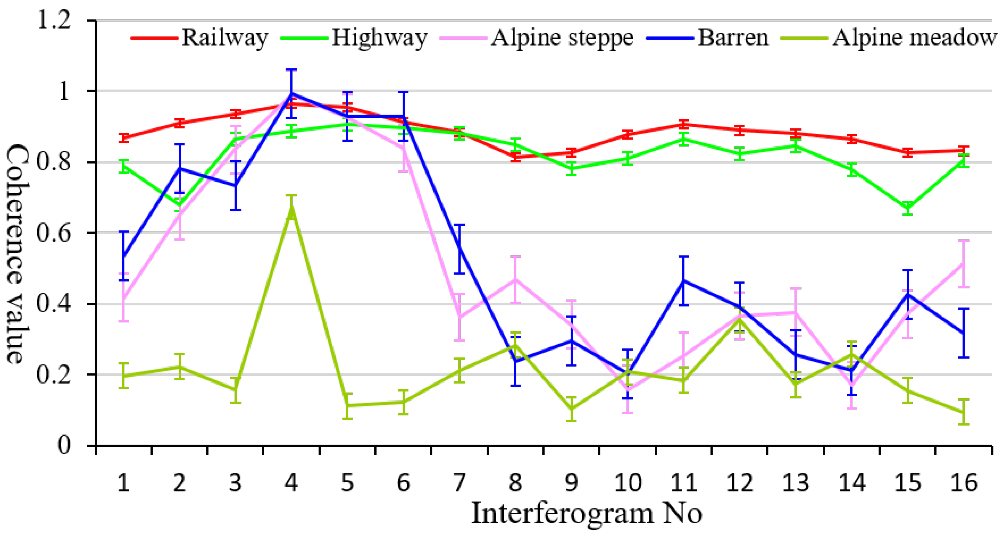
Figure 7 gives the coherence variation for typical ground targets for the CMG. Typical landscapes show different seasonal coherence variation features. The railway and highway areas show the highest coherence (coherence value > 0.8) during the whole observation. However, there is a clear drop in coherence with a long temporal baseline. The seasonal variation of railway and highway coherence is not obvious. The mountain slope and barren areas show medium levels of coherence, which are approximately 0.4. The coherence value in mountain slopes and barren areas show obvious seasonal features. In the winter–winter combination, the mountain slope and barren area shows a high coherence value. With long temporal baseline, the coherence value drops clearly even in the winter–winter combination. The alpine meadow area shows the lowest coherence value, which is less than 0.25. Even in the winter–winter combination, the interferometric coherence map shows a low value in the alpine meadow area.
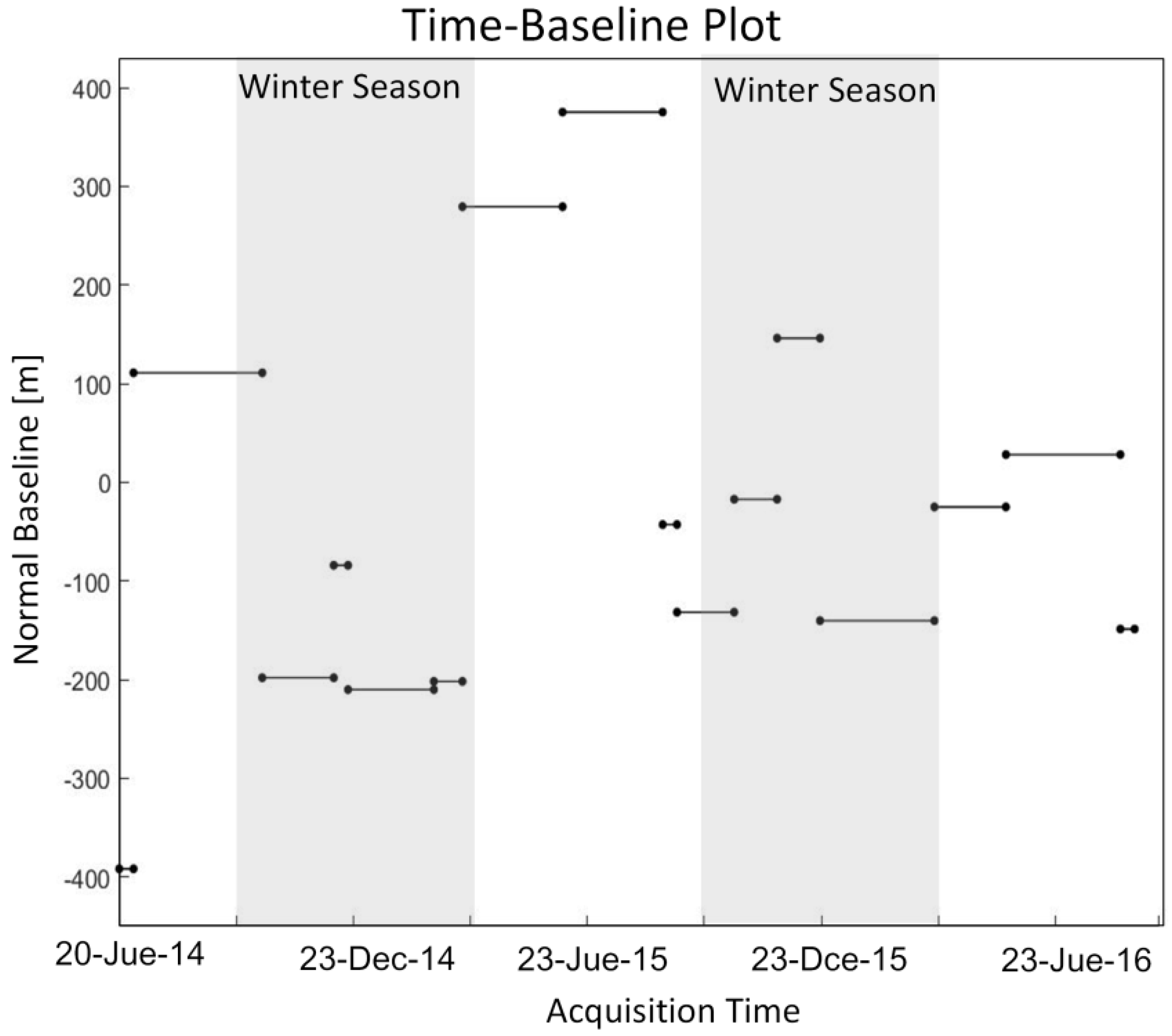
Figure 8 shows the spatial and temporal baseline for the SMG coherences. In the SMG, all the spatial baselines were less than 400 m. Consistent summer–summer, summer–winter and winter–winter interferometric combinations were obtained.
Time-series coherence maps of the study area for the SMG are shown in Figure 9. It is apparent that the mean coherence value of the study area in the SMG is higher than that in the CMG. This occurs because the temporal baseline of the SMG interferometric coherence is smaller than that of the CMG interferometric coherence, which suggests that the temporal baseline is the main factor causing decorrelation in that area. When the master image and slave image are both acquired either in the winter or summer seasons, the resultant coherence map is of high quality. When the master image and slave image are acquired in difference seasons, the coherence map would show serious decorrelation because of the surface environment changes occurring during the observation.
The coherence variation for typical ground targets for SMG interferometric coherence analysis is displayed in Figure 10. In the SMG coherence maps, the study area shows seasonal variation, but different from that in the CMG interferometric coherence maps. The railway and highway areas show a high coherence value (larger than 0.8) in SMG, the same pattern as in the CMG. Coherence maps in mountain slope and barren areas exhibit seasonal changing patterns. When the master and slave images are acquired in the same season, the coherence maps for the mountain slope and barren areas show high values (0.7–0.8). Coherence maps of the alpine meadow area show similar seasonal changes as mountain slope and barren areas, but with lower coherence values (0.6–0.2). It should be noted that the temporal baseline of each interferometric SMG pair is not uniform, which would inflect the result.
From the result of CMG and SMG interferometric coherence maps, it can be concluded that the temporal decorrelation of the study area is correlated with two factors: the long-term temporal baseline and the seasonal-term baseline. Those two decorrelations are consistent with the deformation pattern of the permafrost. Numerous studies have found that the deformation of the permafrost can be expressed as a sum of a linear long-deformation term and a seasonal-deformation term [14,19]. To analyze the temporal coherence, a temporal decorrelation is proposed and presented in the next section.
4.2. Modelling of Temporal Decorrelation
The SAR image acquired on 2 December 2014 was selected as the master image, and 13 interferometric pairs were generated, similar to the CMG processing as described in Section 4.1. The temporal decorrelation of typical ground targets was modelled, as shown in Figure 11. We can observe that most ground targets fit the new temporal decorrelation model except for the alpine meadow area. The retrieved parameters of the model are shown in Table 4. Parameter a and b represent the effects of long-term temporal decorrelation and seasonal temporal decorrelation components, respectively. Parameter c represents the initial coherence value of the first two images, which is correlated with the first interferometric pair.
For the railway target, parameters a and b are −1.11 × 10⁴ and 0.033, respectively. These parameter values are small, an indication that long-term and seasonal temporal decorrelations show little effect on interferometric coherence of the railway. The highway area shows similar performance as the railway area. Thus, railway and highway can maintain a high coherence value even with temporal baseline of several years. For mountain slope and barren areas, parameters a and b are approximately −9 × 10⁻⁴ and 0.1, respectively. Those two parameters are both larger than those of the railway and highway, which suggests that mountain slope and barren areas are more vulnerable to long-term and seasonal-temporal decorrelations. The coherence values of the mountain slope and barren areas are less than 0.2 when the temporal baselines are longer than two years. For the alpine meadow area, the temporal decorrelation is the most serious and there is no seasonal variation of the coherence. The coherence value of the alpine meadow area is consistently low during the observation.
5. Discussion
In the QTP area, the coherence of typical ground targets shows obvious seasonal variation, which is consistent with the results of previous stuies conducted in other permafrost areas [22]. Except for the effect of a large spatial baseline, we attribute those decorrelations to the surface changes between the master and slave image. In this section, the enviornmental factors and human activities affecting the coherence are discussed based on previous studies and field investigations.
5.1. Effect of Vegetation
Vegetation growth or decline over two time points will contribute to serious temporal decorrelation. Dense vegetation results in greater decorrelation than sparse vegetation during the same timespan, which makes classification or change detection possible. Several studies used the coherence information for land-cover classification or change detection [21,34]. Within our study region, an alpine meadow area lies in the south west of the test site (Figure 2c). Other areas can be seen as barren areas. The alpine meadow grows in the summer and withers in the winter.
In this study, the barren areas hold higher coherence values than the alpine meadow areas, which is consistent with that fact that greater biomass leads to stronger decorrelation [23]. Figure 12 shows the coherence difference between alpine meadow and alpine desert. For the alpine meadow area in box “1” the mean coherence value is about 0.27, while the mean coherence value in the alpine desert is about 0.47. Moreover, the state of vegetation would change the coherence value. The alpine meadow area yields lower coherence values in the summer season than in the winter season. This is because the vegetation have withered in winter, and the volume-scattering of the surface is weak. In the summer season, the vegetaion grows with the incease of soil moisure, which contributes to serious decorrelation.
5.2. Effect of Soil Moisture
The relationship between soil moisture and InSAR coherence and phase has been recognized since 1989 [35]. Subsequently, many studies and models have been conducted and proposed to relate soil moisture and InSAR coherence [36,37,38]. De Zan et al., 2014 provided a new explanation for interferometric phases and coherences and validated it with real L-band data over bare surfaces [36]. Zwieback et al., 2017 found that the DInSAR phase can be a suitable means to estimate soil moisture time series up to an overall offset, as indicated by correlations with in situ measurements of 0.75–0.90 in two campaigns [38].
However, there was a lack of clear evidence for the contribution of soil-moisture change to decorrelation in our study. It should be noted that in an area near drainage, the soil moisture is higher than other areas, as revealed through field investigations. Moreover, the coherence in such areas is lower than that in other areas. The state of the soil moisture in the active layer varies with the temperature, which makes the frost soil more special. To analyze the relationship between soil moisture and InSAR coherence, soil moisture should be measured and used to build a model. Futher work will focus on elucidating the effect of soil moisture on interferometric coherence.
5.3. Effect of Active Layer (AL) Freezing and Thawing
In our permafrost study area, the thawing date is approximately 15 April and freezing of the soil begins on the 1 October [2]. The freezing and thawing cycle changes the state of the water in the soil, which would change the volume and water content therein. The active layer thawing in the summer season results in ground water 9% less in volume than ground ice in the permafrost layer [15]. Deformation from the volume loss of soil layer may cause serious decorrelation due to ground-surface changes.
In our study, in the winter season, the mean coherence value in the interferometric pair of 20150217–20150311 is greater than that of other interferometric pairs of 20141202–20141213 in the SMG (Figure 9). It is more obvious in alpine mdeadow area. In Figure 8, the coherence value of the selcted point is 0.67 in the interferometric pair (20141202–20141213) and 0.87 in the interferometric pair (20150217–20150311). This may be explained by considering that in the permafrost area, at the begining of the freezing cycle, the AL freezes significantly and quickly, which cause large the deformation and surface change, which contribute to low coherence at that stage. At the end of the freezing cycle, the AL freezes completely, the permafrost becomes more stable, and the surface changes little, which results in greater coherence value [10].
5.4. Effect of Human Activity
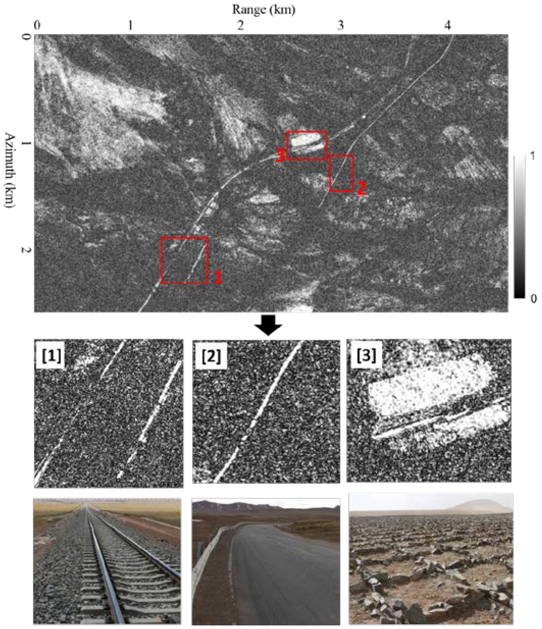
When the QTR was completed, human activities become more frequent in the QTP. Numerous engineered structures have been constructed on the QTP, which have changed the condition of the permafrost. Due to the strong backscattering, those structures can also be reflected in the InSAR coherence map. Tang et al., 2013 analyzed the coherence of railway and highway using ASAR images [33]. In our study, three typical engineered structures ( representation of human activity), such as railway, highway and soil-control measurements, were selectied and their coherence values were analyzed (Figure 13). As shown in Figure 13, most parts of the areas show low coherence, except for the engineered portions. Pixels of those engineered structures in the SAR image are strong backscatters points, which can hold high coherence during the long term. Those man-made engineering works could be selected as the persistent scatter for demformation monitoring of the QTP using time-series InSAR, which we will focus on in further work.
Thus, if the time-series InSAR technique is used to monitor the deformation in permafrost areas with TerraSAR images, the temporal baseline is ideally set to less than one year. When monitoring the deformation of the human engineered structure, the temporal baseline can be set longer than two years.
6. Conclusions
This study is the first to analyze the coherence variation of permafrost in the QTP using high-resolution SAR images. Time-series coherence maps of the study area were obtained. The experimental results show that railway and highway hold high coherence during the whole observation, with the maximum coherence value greater than 0.8. Those high-coherence points could be used for the deformation monitoring of the QTP using time-series InSAR. On the mountain slope, barren and alpine meadow areas, the coherence shows obvious seasonal variation. A new temporal decorrelation model is proposed herein for permafrost areas. Most typical ground targets fit the temporal-decorrelation model determined by a linear temporal-decorrelation component and a seasonal periodic-decorrelation component and a constant component. In this study, railway and highway can hold high coherence even with the temporal baseline over several years with X-band SAR data. By contrast, after one single annual cycle, the coherence of the mountain slope and barren areas is less than 0.2. Possible factors affecting the InSAR coherence (vegetation, soil moisture, soil freezing and thawing, and human activity) have been discussed herein. Temperature and soil moisture are the main factors determining the coherence condition of the ground surface. In the summer season, with the increase of temperature, the frozen active layer begins to thaw and the soil moisture increases. The vegetation morphology changes rapidly, which contributes to serious decorrelation, especially in the alpine meadow area. In the winter season, with the decrease of temperature, the soil is in a dry condition and the scattering of the ground surface could remain in a stable condition. This study suggests that high-resolution SAR coherence map could provide a new tool for studying permafrost environmental conditions.
Future work will focus on soil-moisture retrieving and the relationship between the coherence variation and soil moisture, as well as on the assessment of the deformation of the permafrost region using time-series InSAR.
Acknowledgments
This work was supported by the project of TerraSAR-X New Modes AO (ID: HYD2420), and funded the National Natural Science Foundation of China under Grant 41331176. All TerraSAR-X data was provided by DLR. Bo Zhang, Meng Liu, Fan Wu, Lei Xie, Jinxing Chen, Mingzhe Zhang, Tianzheng Wang participated in the field work.
Author Contributions
Chao Wang conceived and designed the experiments; Zhengjia Zhang performed the experiments and wrote the paper; Hong Zhang and Yixian Tang performed the data analysis and interpretation of the results; Xiuguo Liu edited the final manuscript.
Conflicts of Interest
The authors declare no conflict of interest.
References
- Harris, S.; French, H.; Heginbottom, J.; Johnston, G.; Ladanyi, B.; Sego, D.; van Everdingen, R. Glossary of Permafrost and Related Ground-Ice Terms; Technical Memorandum 142; National Research Council of Canada: Ottawa, ON, Canada, 1988. [Google Scholar]
- Wu, Q.B.; Hou, Y.D.; Yun, H.B.; Liu, Y.Z. Changes in active-layer thickness and near-surface permafrost between 2002 and 2012 in alpine ecosystems, Qinghai–Xizang (Tibet) Plateau, China. Glob. Planet. Chang. 2015, 124, 149–155. [Google Scholar] [CrossRef]
- Zhao, L.; Wu, Q.B.; Marchenko, S.S.; Sharkhuu, N. Thermal state of permafrost and active layer incentral Asia during the International Polar Year. Permafr. Periglac. 2010, 21, 198–207. [Google Scholar] [CrossRef]
- Subcommittee, Permafrost. Glossary of Permafrost and Related Ground-Ice Terms; Technical Memorandum; National Research Council of Canada: Ottawa, ON, Canada, 1988. [Google Scholar]
- Chen, F.L.; Lin, H.; Zhou, W.; Hong, T.H.; Wang, G. Surface deformation detected by ALOS PALSAR small baseline SAR interferometry over permafrost environment of Beiluhe section, Tibet Plateau, China. Remote Sens. Environ. 2013, 138, 10–18. [Google Scholar] [CrossRef]
- Cheng, G.; Wu, T. Responses of permafrost to climate change and their environmental significance, Qinghai-Tibet Plateau. J. Geophys. Res. 2007, 112. [Google Scholar] [CrossRef]
- Guo, D.; Wang, H. Simulation of permafrost and seasonally frozen ground conditions on the Tibetan Plateau, 1981–2010. J. Geophys. Res. 2013, 118, 5216–5230. [Google Scholar] [CrossRef]
- Lin, Z.J.; Niu, F.J.; Luo, J.; Lu, J.H.; Liu, H. Changes in permafrost environments caused by construction and maintenance of Qinghai-Tibet Highway. J. Cent. South Univ. Technol. 2011, 18, 1454–1464. [Google Scholar] [CrossRef]
- Pang, Q.; Cheng, G.; Li, S.X.; Zhang, W.G. Active layer thickness calculation over the Qinghai–Tibet Plateau. Cold Reg. Sci. Technol. 2009, 57, 23–28. [Google Scholar] [CrossRef]
- Wu, Q.B.; Niu, F.J. Permafrost changes and engineering stability in Qinghai-Xizang Plateau. Chin. Sci. Bull. 2013, 58, 1079–1094. [Google Scholar] [CrossRef]
- Ma, W.; Mu, Y.; Wu, Q.B.; Sun, Z.Z.; Liu, Y.Z. Characteristics and mechanisms of embankment deformation along the Qinghai–Tibet Railway in permafrost regions. Cold Reg. Sci. Technol. 2011, 67, 178–186. [Google Scholar] [CrossRef]
- Niu, F.J.; Lin, Z.; Lu, J.H.; Liu, H.; Xu, Z.Y. Characteristics of roadbed settlement in embankment–bridge transition section along the Qinghai-Tibet Railway in permafrost regions. Cold Reg. Sci. Technol. 2011, 65, 437–445. [Google Scholar] [CrossRef]
- Li, S.Y.; Lai, Y.M.; Zhang, M.Y.; Dong, Y.H. Study on long-term stability of Qinghai–Tibet Railway embankment. Cold Reg. Sci. Technol. 2009, 57, 139–147. [Google Scholar] [CrossRef]
- Li, Z.; Tang, P.; Zhou, J.; Tian, B.; Chen, Q.; Fu, S. Permafrost environment monitoring on the Qinghai-Tibet Plateau using time series ASAR images. Int. J. Digit. Earth 2014, 8, 1–21. [Google Scholar] [CrossRef]
- Wang, C.; Zhang, Z.J.; Zhang, H.; Wu, Q.B.; Zhang, B.; Tang, Y.X. Seasonal deformation features on Qinghai-Tibet railway observed using time-series InSAR technique with high-resolution TerraSAR-X images. Remote Sens. Lett. 2017, 1, 1–10. [Google Scholar] [CrossRef]
- Li, Z.; Zhao, R. Monitoring surface deformation over permafrost with an improved SBAS-InSAR algorithm: With emphasis on climatic factors modeling. Remote Sens. Environ. 2016, 184, 276–287. [Google Scholar]
- Ferretti, A.; Prati, C.; Rocca, F. Permanent scatterers in SAR interferometry. IEEE Trans. Geosci. Remote Sens. 2001, 39, 8–20. [Google Scholar] [CrossRef]
- Hooper, A.; Zebker, H.; Segall, P.; Kampes, B. A new method for measuring deformation on volcanoes and other natural terrains using InSAR persistent scatterers. Geophys. Res. Lett. 2004, 31. [Google Scholar] [CrossRef]
- Berardino, P.; Fornaro, G.; Lanari, R.; Sansosti, E. A new algorithm for surface deformation monitoring based on small baseline differential SAR interferograms. IEEE Trans. Geosci. Remote Sens. 2002, 40, 2375–2383. [Google Scholar] [CrossRef]
- Lanari, R.; Mora, O.; Manunta, M.; MallorquíJ, J.; Berardino, P.; Sansosti, E. A small-baseline approach for investigating deformations on full-resolution differential SAR interferograms. IEEE Trans. Geosci. Remote Sens. 2004, 42, 1377–1386. [Google Scholar] [CrossRef]
- Chen, F.; Guo, H.; Ishwaran, N.; Zhou, W.; Yang, R.; Jing, L.; Zeng, H. Synthetic aperture radar (SAR) interferometry for assessing Wenchuan earthquake (2008) deforestation in the Sichuan giant panda site. Remote Sens. 2014, 6, 6283–6299. [Google Scholar] [CrossRef]
- Wickramanayake, A.; Henschel, M.D.; Hobbs, S.; Buehler, S.A.; Ekman, J.; Lehrbass, B. Seasonal variation of coherence in SAR interferograms in Kiruna, Northern Sweden. Int. J. Remote Sens. 2016, 2, 370–387. [Google Scholar]
- Antonova, S.; Kääb, A.; Heim, B.; Langer, M.; Boike, J. Spatio-temporal variability of X-band radar backscatter and coherence over the Lena River Delta, Siberia. Remote Sens. Environ. 2016, 182, 169–191. [Google Scholar] [CrossRef]
- Jung, H.C.; Alsdorf, D. Repeat-Pass Multi-Temporal Interferometric SAR Coherence Variations with Amazon Floodplain and Lake Habitats. Int. J. Remote Sens. 2010, 31, 881–901. [Google Scholar] [CrossRef]
- Weydahl, D. Analysis of ERS Tandem SAR Coherence from Glaciers, Valleys, and Fjord Ice on Svalbard. IEEE Trans. Geosci. Remote Sens. 2001, 39, 2029–2039. [Google Scholar] [CrossRef]
- Zebker, H.A.; Villasenor, J. Decorrelation in interferometric radar echoes. IEEE Trans. Geosci. Remote Sens. 1992, 30, 950–959. [Google Scholar] [CrossRef]
- Wei, M.; Sandwell, D.T. Decorrelation of L-band and C-band interferometry over vegetated areas in California. IEEE Trans. Geosci. Remote Sens. 2010, 48, 2942–2952. [Google Scholar]
- Wang, T.; Liao, M.; Perissin, D. InSAR coherence-decomposition analysis. IEEE Geosci. Remote Sens. Lett. 2010, 7, 156–160. [Google Scholar] [CrossRef]
- Hoen, E.W.; Zebker, H.A. Penetration depths inferred from interferometric volume decorrelation observed over the Greenland ice sheet. IEEE Trans. Geosci. Remote Sens. 2010, 38, 2571–2583. [Google Scholar]
- Guarnieri, A.M.; Tebaldini, S. Hybrid Cramér–Rao bounds for crustal displacement field estimators in SAR interferometry. IEEE Signal Proc. Lett. 2007, 14, 1012–1015. [Google Scholar] [CrossRef]
- Rossi, C.; Minet, C.; Fritz, T.; Eineder, M.; Bamler, R. Temporal monitoring of subglacial volcanoes with TanDEM-X—Application to the 2014–2015 eruption within the Bárðarbunga volcanic system, Iceland. Remote Sens. Environ. 2016, 181, 186–197. [Google Scholar] [CrossRef]
- Tang, P.; Zhou, W.; Tian, B.; Chen, F.; Li, Z.; Li, G. Quantification of temporal decorrelation in x-, c-, and l-band interferometry for the permafrost region of the qinghai-tibet plateau. IEEE Geosci. Remote Sens. Lett. 2017, 99, 1–5. [Google Scholar] [CrossRef]
- Tang, P.P.; Li, Z.; Zhou, J.M.; Tian, B.S.; Xu, J. Coherence based analysis of distributed scatterers in the Qinghai-Tibet Plateau. In Proceedings of the 2013 IEEE International Geoscience and Remote Sensing Symposium (IGARSS), Melbourne, Australia, 21–26 July 2013; pp. 1356–1359. [Google Scholar]
- Kubanek, J.; Westerhaus, M.; Schenk, A.; Aisyah, N.; Brotopuspito, K.S.; Heck, B. Volumetric change quantification of the 2010 Merapi eruption using TanDEM-X InSAR. Remote Sens. Environ. 2015, 164, 16–25. [Google Scholar] [CrossRef]
- Gabriel, A.; Goldstein, R.; Zebker, H. Mapping small elevation changes over large areas: Differential radar interferometry. J. Geophys. Res. 1989, 94, 9183–9191. [Google Scholar] [CrossRef]
- De Zan, F.; Parizzi, A.; Prats-Iraola, P.; López-Dekker, P. A SAR interferometric model for soil moisture. IEEE Trans. Geosci. Remote Sens. 2014, 52, 418–425. [Google Scholar] [CrossRef] [Green Version]
- Zwieback, S.; Hensley, S.; Hajnsek, I. Assessment of soil moisture effects on L-band radar interferometry. Remote Sens. Environ. 2015, 164, 77–89. [Google Scholar] [CrossRef] [Green Version]
- Zwieback, S.; Hensley, S.; Hajnsek, I. Soil Moisture Estimation Using Differential Radar Interferometry: Toward Separating Soil Moisture and Displacements. IEEE Trans. Geosci. Remote Sens. 2017, 55, 5069–5083. [Google Scholar] [CrossRef]
Figure 1.
(a) Air temperature; (b) monthly precipitation.
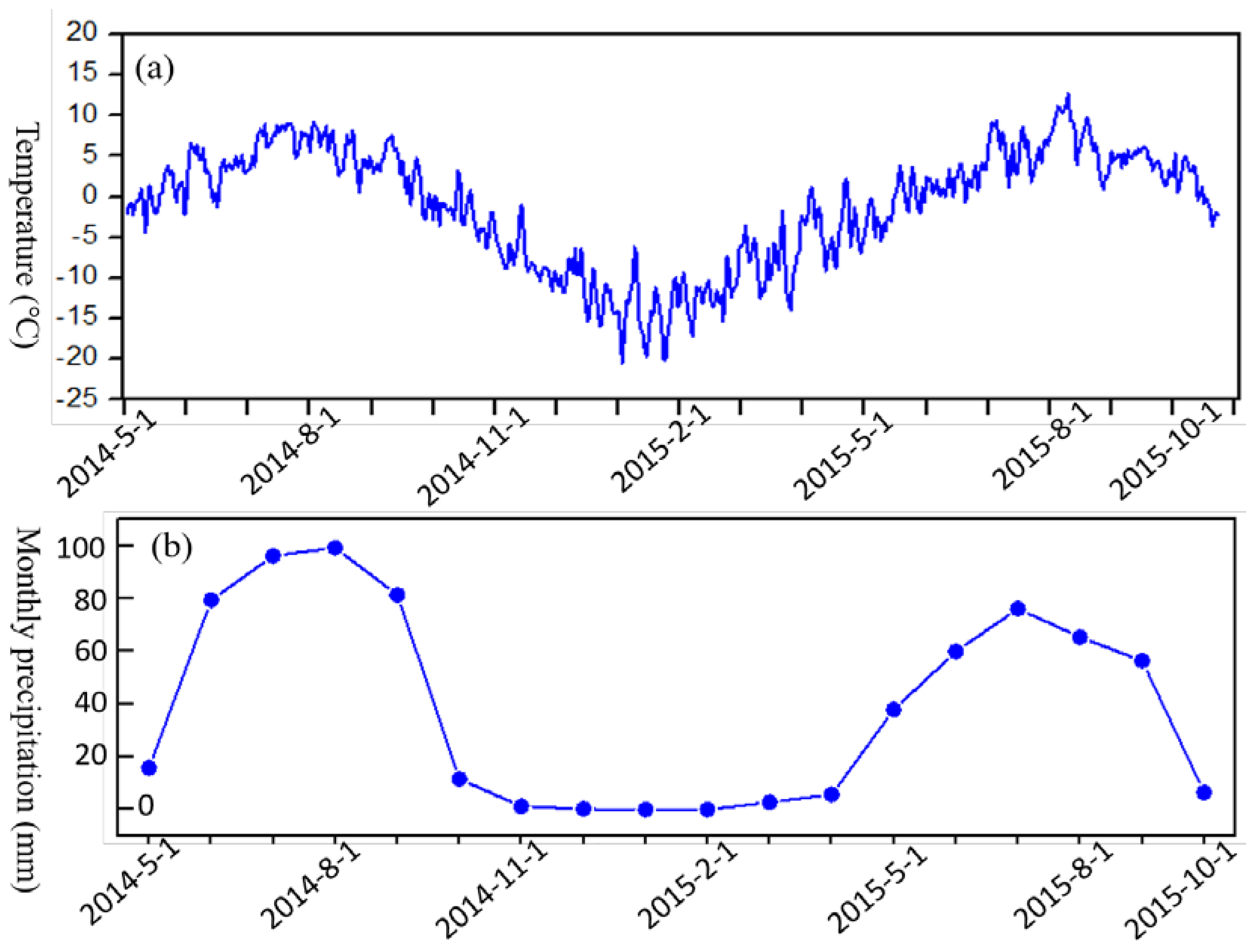
Figure 2.
(a) Location of Beiluhe area of Qinghai province, China. (b) The Shuttle Radar Topography Mission (SRTM) digital elevation model (DEM) of the study area. The colored frame indicates the ground coverage of the SAR image. (c) The Google map imagery of the study area.
Figure 2.
(a) Location of Beiluhe area of Qinghai province, China. (b) The Shuttle Radar Topography Mission (SRTM) digital elevation model (DEM) of the study area. The colored frame indicates the ground coverage of the SAR image. (c) The Google map imagery of the study area.

Figure 3.
Field photos of the typical ground targets in the winter and summer seasons.

Figure 4.
The location of the selected samples.

Figure 5.
Spatial and temporal baseline for the common master group (CMG). The black dot denotes the synthetic aperture radar (SAR) images. The black line indicates the interferometric pair.
Figure 5.
Spatial and temporal baseline for the common master group (CMG). The black dot denotes the synthetic aperture radar (SAR) images. The black line indicates the interferometric pair.
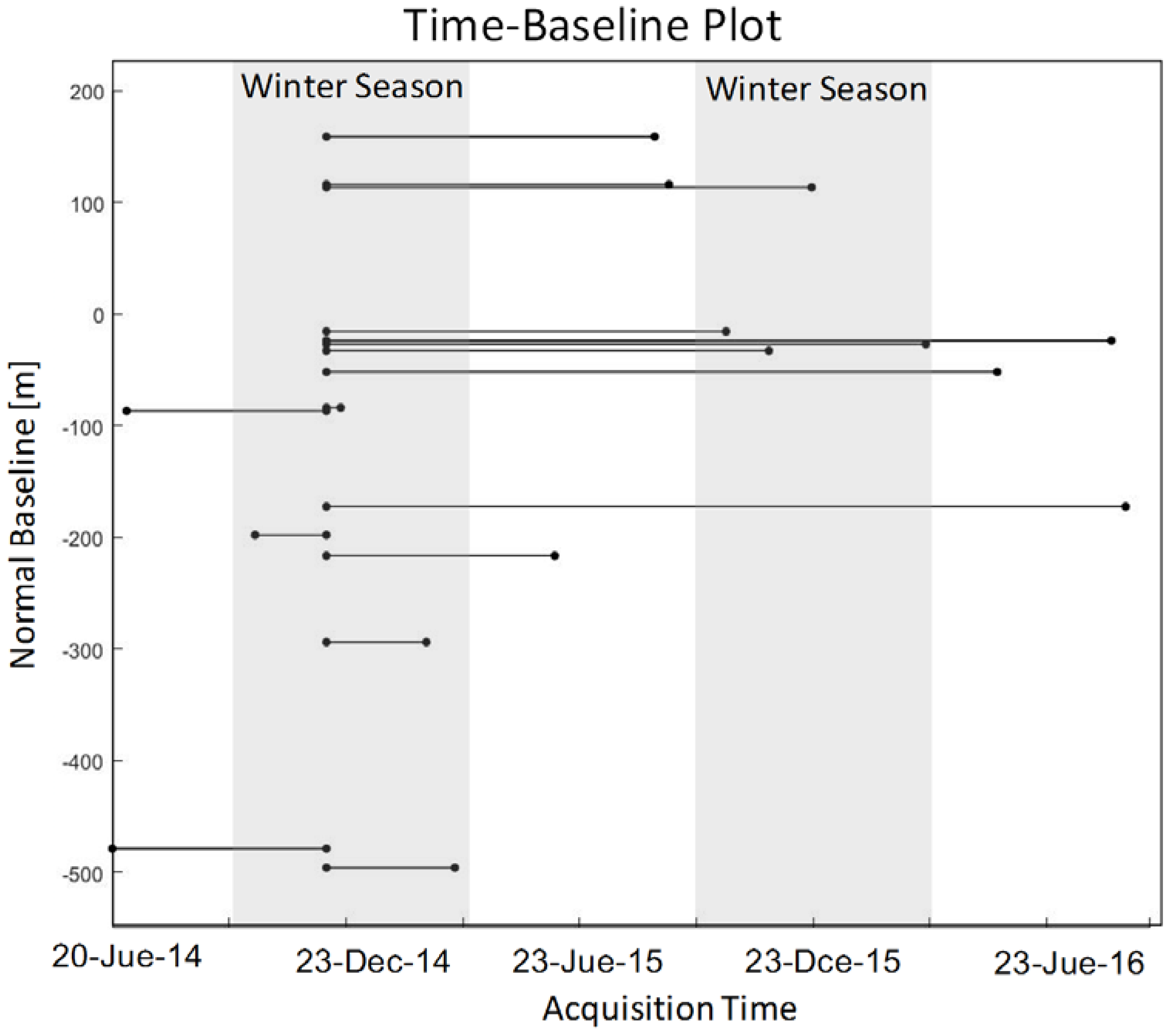
Figure 6.
Time-series coherence maps of the study area for the CMG. The image acquired in the winter season (2 December 2014) is selected as the master image.
Figure 6.
Time-series coherence maps of the study area for the CMG. The image acquired in the winter season (2 December 2014) is selected as the master image.

Figure 7.
Coherence variation for typical ground targets in the CMG.

Figure 8.
Spatial and temporal baseline for the sequential master group (SMG). The black dot denotes the SAR image. The black line indicates the interferometric pair.
Figure 8.
Spatial and temporal baseline for the sequential master group (SMG). The black dot denotes the SAR image. The black line indicates the interferometric pair.

Figure 9.
Time-series coherence maps of the study area for the SMG.
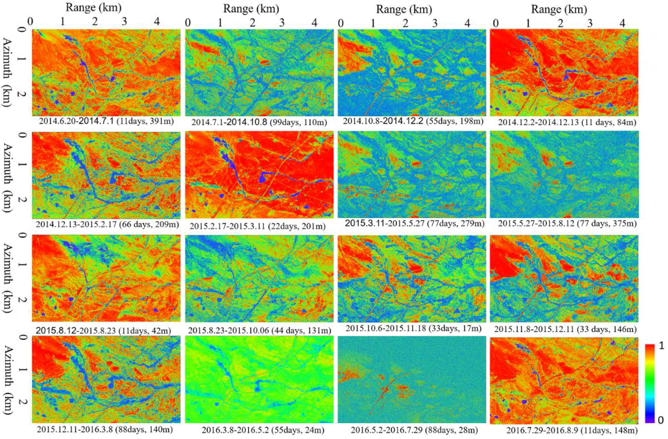
Figure 10.
Coherence variation for typical ground targets in the SMG.
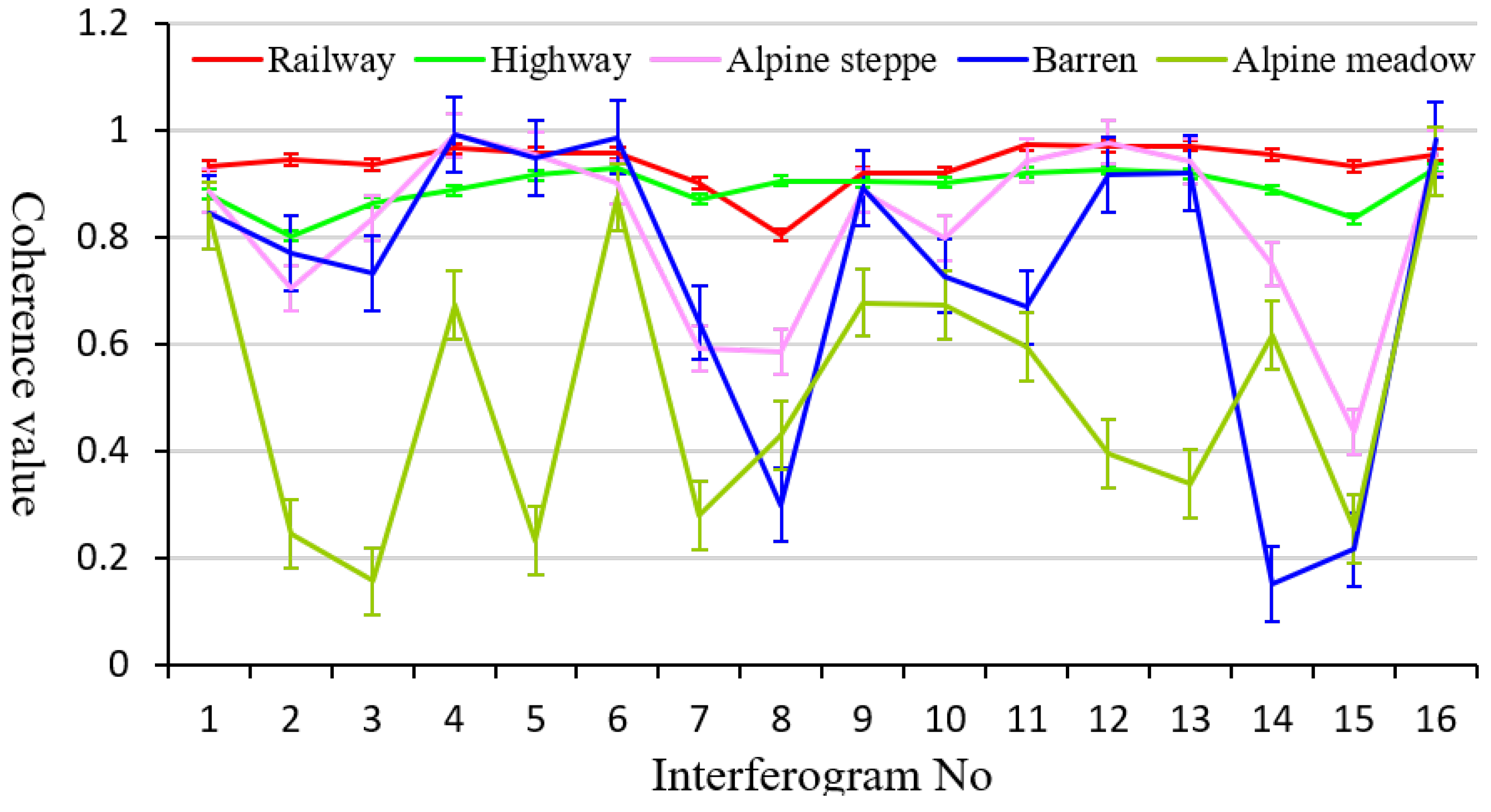
Figure 11.
Temporal decorrelation modelling of different ground targets: railway (a); highway (b); mountain slope (c); barren (d); and alpine meadow (e).
Figure 11.
Temporal decorrelation modelling of different ground targets: railway (a); highway (b); mountain slope (c); barren (d); and alpine meadow (e).
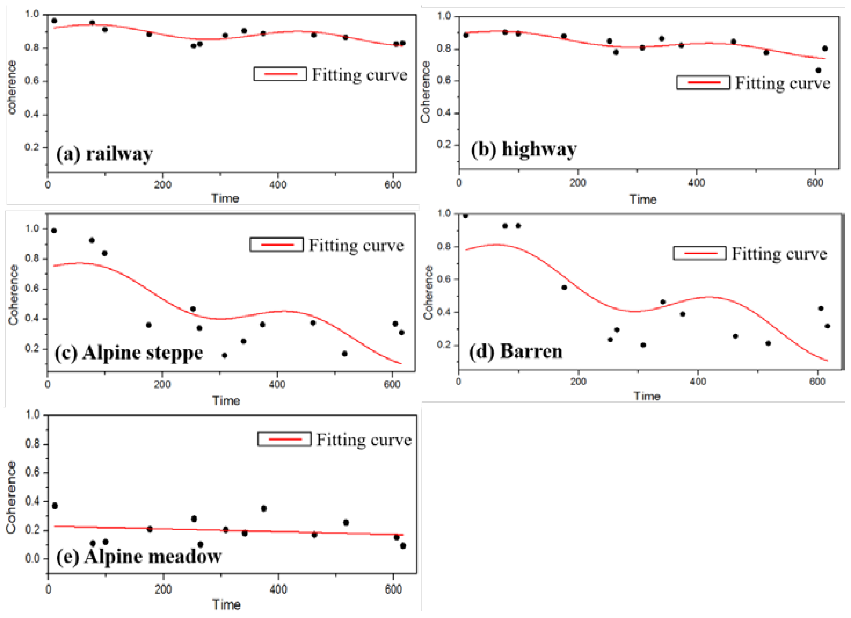
Figure 12.
(a) Coherence of interferometric pair 20140601–20141202. box “1” and “2” are the alpine meadow and desert areas, respectively; (b,c) are the histogram plot of alpine meadow and desert area in box “1” and “2”.
Figure 12.
(a) Coherence of interferometric pair 20140601–20141202. box “1” and “2” are the alpine meadow and desert areas, respectively; (b,c) are the histogram plot of alpine meadow and desert area in box “1” and “2”.
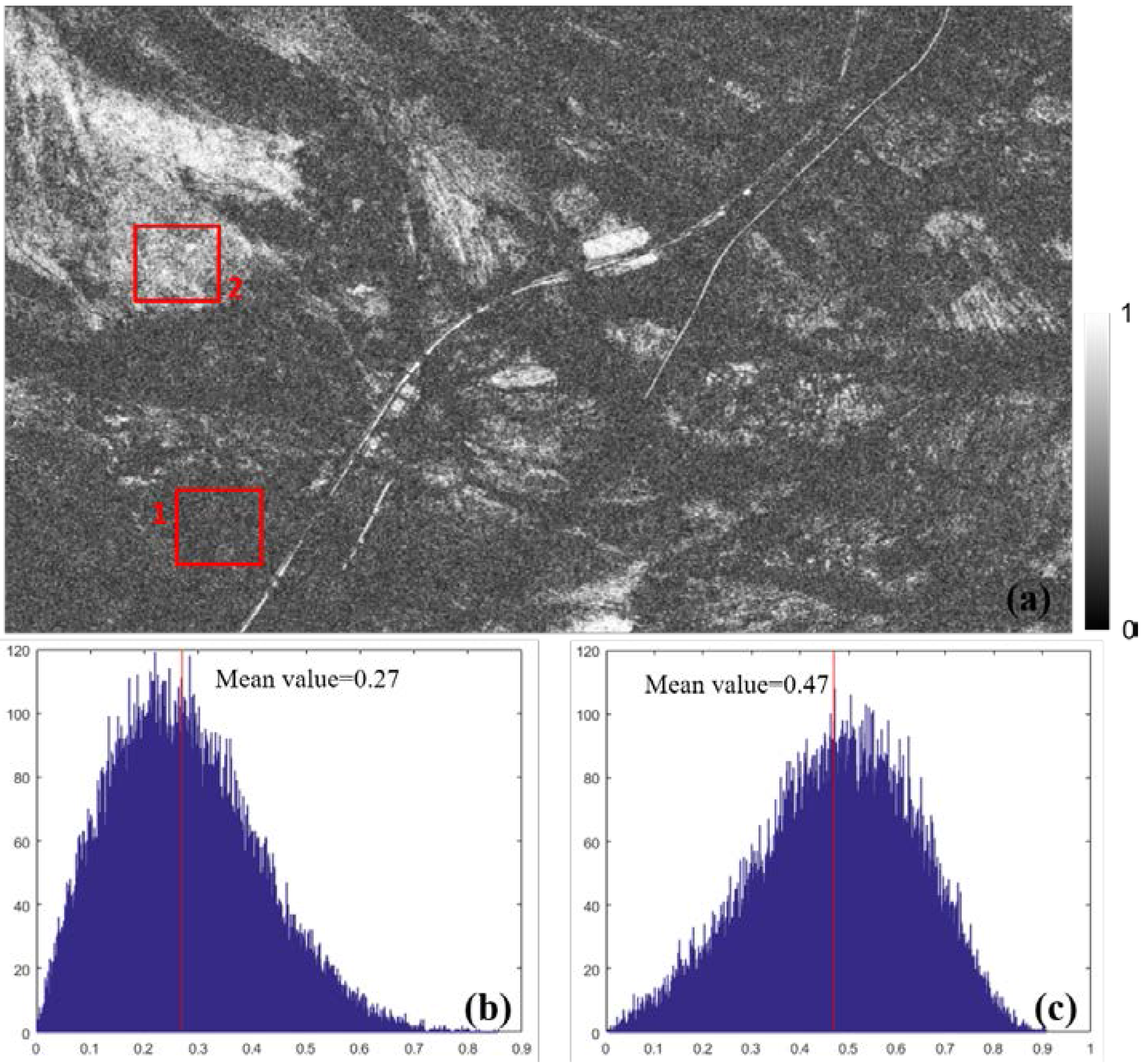
Figure 13.
Coherence of interferometric pair 20140601–20141202. Boxes “1”, “2”, and “3”are railway, highway, and soil-control measurements, all reflecting human activity.
Figure 13.
Coherence of interferometric pair 20140601–20141202. Boxes “1”, “2”, and “3”are railway, highway, and soil-control measurements, all reflecting human activity.

Table 1.
TerraSAR-X image parameters.
| Image Number | Acquisition Date | Normal Baseline (m) | Temporal Baseline (Day) | Thawing (T)/Freezing (F) Season |
|---|---|---|---|---|
| 1 | 20 June 2014 | 0 | 0 | T |
| 2 | 1 July 2014 | 391 | 11 | T |
| 3 | 8 October 2014 | 280 | 110 | F |
| 4 | 2 December 2014 | 478 | 165 | F |
| 5 | 13 December 2014 | 562 | 176 | F |
| 6 | 17 February 2015 | 772 | 242 | F |
| 7 | 11 March 2015 | 974 | 264 | F |
| 8 | 27 May 2015 | 695 | 341 | T |
| 9 | 12 August 2015 | 320 | 418 | T |
| 10 | 23 August 2015 | 362 | 429 | T |
| 11 | 6 October 2015 | 494 | 473 | F |
| 12 | 8 November 2015 | 511 | 506 | F |
| 13 | 11 December 2015 | 365 | 539 | F |
| 14 | 8 March 2016 | 505 | 627 | F |
| 15 | 2 May 2016 | 530 | 682 | T |
| 16 | 29 July 2016 | 502 | 770 | T |
| 17 | 9 October 2016 | 651 | 781 | T |
Table 2.
Common master interferograms.
| Int a No | Master Image | Slave Image | Normal Baseline (m) | Temporal Baseline (Day) | Acquisition Season b | Acquisition Season c |
|---|---|---|---|---|---|---|
| 1 | 2 December 2014 | 20 June 2014 | 478 | −165 | Winter | Summer |
| 2 | 2 December 2014 | 1 July 2014 | 87 | −147 | Winter | Summer |
| 3 | 2 December 2014 | 8 October 2014 | 198 | −55 | Winter | Summer |
| 4 | 2 December 2014 | 13 December 2014 | 84 | 11 | Winter | Winter |
| 5 | 2 December 2014 | 17 February 2015 | 294 | 77 | Winter | Winter |
| 6 | 2 December 2014 | 11 March 2015 | 495 | 99 | Winter | Winter |
| 7 | 2 December 2014 | 27 May 2015 | 216 | 176 | Winter | Summer |
| 8 | 2 December 2014 | 12 August 2015 | 158 | 253 | Winter | Summer |
| 9 | 2 December 2014 | 23 August 2015 | 115 | 264 | Winter | Summer |
| 10 | 2 December 2014 | 6 October 2015 | 15 | 308 | Winter | Summer |
| 11 | 2 December 2014 | 8 November 2015 | 32 | 341 | Winter | Winter |
| 12 | 2 December 2014 | 11 December 2015 | 113 | 374 | Winter | Winter |
| 13 | 2 December 2014 | 8 March 2016 | 27 | 462 | Winter | Winter |
| 14 | 2 December 2014 | 2 May 2016 | 52 | 517 | Winter | Summer |
| 15 | 2 December 2014 | 29 July 2016 | 23 | 605 | Winter | Summer |
| 16 | 2 December 2014 | 9 October 2016 | 172 | 616 | Winter | Summer |
Note: a for interferogram number; b for master image; c for slave image.
Table 3.
Sequential master interferograms.
| Int a No | Master Image | Slave Image | Normal Baseline (m) | Temporal Baseline (Day) | Acquisition Season b | Acquisition Season c |
|---|---|---|---|---|---|---|
| 1 | 20 June 2014 | 1 July 2014 | 391 | 11 | Summer | Summer |
| 2 | 1 July 2014 | 8 October 2014 | 110 | 99 | Summer | Summer |
| 3 | 8 October 2014 | 2 December 2014 | 198 | 55 | Summer | Winter |
| 4 | 2 December 2014 | 13 December 2014 | 84 | 11 | Winter | Winter |
| 5 | 13 December 2014 | 17 February 2015 | 209 | 66 | Winter | Winter |
| 6 | 17 February 2015 | 11 March 2015 | 201 | 22 | Winter | Winter |
| 7 | 11 March 2015 | 27 May 2015 | 279 | 77 | Winter | Summer |
| 8 | 27 May 2015 | 12 August 2015 | 375 | 77 | Summer | Summer |
| 9 | 12 August 2015 | 23 August 2015 | 42 | 11 | Summer | Summer |
| 10 | 23 August 2015 | 6 October 2015 | 131 | 44 | Summer | Summer |
| 11 | 6 October 2015 | 8 November 2015 | 17 | 33 | Summer | Winter |
| 12 | 8 November 2015 | 11 December 2015 | 146 | 33 | Winter | Winter |
| 13 | 11 December 2015 | 8 March 2016 | 140 | 88 | Winter | Winter |
| 14 | 8 March 2016 | 2 May 2016 | 24 | 55 | Winter | Summer |
| 15 | 2 May 2016 | 29 July 2016 | 28 | 88 | Summer | Summer |
| 16 | 29 July 2016 | 9 October 2016 | 148 | 11 | Summer | Summer |
Note: a for interferogram number; b for master image; c for slave image.
Table 4.
Parameters of the decorrelation model for different land cover types.
| Land Cover Type | a | b | c | R2 | RMSE |
|---|---|---|---|---|---|
| Railway | −1.11 × 10⁻⁴ | 0.033 | 0.917 | 0.66 | 0.0224 |
| Highway | −2.08 × 10⁻⁴ | 0.028 | 0.899 | 0.62 | 0.0345 |
| Mountain slope | −9.002 × 10⁻⁴ | 0.091 | 0.74 | 0.52 | 0.176 |
| Barren | −8.82 × 10⁻⁴ | 0.111 | 0.7714 | 0.54 | 0.1716 |
| Alpine meadow | −9.68 × 10⁻⁴ | 2.43 × 10⁻⁴ | 0.223 | 0.14 | 0.086 |
© 2018 by the authors. Licensee MDPI, Basel, Switzerland. This article is an open access article distributed under the terms and conditions of the Creative Commons Attribution (CC BY) license (http://creativecommons.org/licenses/by/4.0/).
Share and Cite
MDPI and ACS Style
Zhang, Z.; Wang, C.; Zhang, H.; Tang, Y.; Liu, X. Analysis of Permafrost Region Coherence Variation in the Qinghai–Tibet Plateau with a High-Resolution TerraSAR-X Image. Remote Sens. 2018, 10, 298. https://doi.org/10.3390/rs10020298
AMA Style
Zhang Z, Wang C, Zhang H, Tang Y, Liu X. Analysis of Permafrost Region Coherence Variation in the Qinghai–Tibet Plateau with a High-Resolution TerraSAR-X Image. Remote Sensing. 2018; 10(2):298. https://doi.org/10.3390/rs10020298
Chicago/Turabian StyleZhang, Zhengjia, Chao Wang, Hong Zhang, Yixian Tang, and Xiuguo Liu. 2018. "Analysis of Permafrost Region Coherence Variation in the Qinghai–Tibet Plateau with a High-Resolution TerraSAR-X Image" Remote Sensing 10, no. 2: 298. https://doi.org/10.3390/rs10020298
Note that from the first issue of 2016, this journal uses article numbers instead of page numbers. See further details here.