A Robust Transform Estimator Based on Residual Analysis and Its Application on UAV Aerial Images


1
School of Computer Engineering, Jimei University, Xiamen 360121, China
2
Fujian Collaborative Innovation Center for Big Data Applications in Governments, Fuzhou 350003, China
3
School of Information Science and Technology, Xiamen University, Xiamen 361000, China
4
School of Mathematics, Northwest University, Xi′an 710127, China
5
State Key Lab of Resources and Environmental Information System, Institute of Geographic Sciences and Natural Resources Research, Chinese Academy of Sciences, Beijing 100101, China
*
Author to whom correspondence should be addressed.
Remote Sens. 2018, 10(2), 291; https://doi.org/10.3390/rs10020291
Submission received: 15 December 2017
/
Revised: 1 February 2018
/
Accepted: 6 February 2018
/
Published: 13 February 2018
(This article belongs to the Special Issue Remote Sensing from Unmanned Aerial Vehicles (UAVs))
Abstract
:Estimating the transformation between two images from the same scene is a fundamental step for image registration, image stitching and 3D reconstruction. State-of-the-art methods are mainly based on sorted residual for generating hypotheses. This scheme has acquired encouraging results in many remote sensing applications. Unfortunately, mainstream residual based methods may fail in estimating the transform between Unmanned Aerial Vehicle (UAV) low altitude remote sensing images, due to the fact that UAV images always have repetitive patterns and severe viewpoint changes, which produce lower inlier rate and higher pseudo outlier rate than other tasks. We performed extensive experiments and found the main reason is that these methods compute feature pair similarity within a fixed window, making them sensitive to the size of residual window. To solve this problem, three schemes that based on the distribution of residuals are proposed, which are called Relational Window (RW), Sliding Window (SW), Reverse Residual Order (RRO), respectively. Specially, RW employs a relaxation residual window size to evaluate the highest similarity within a relaxation model length. SW fixes the number of overlap models while varying the length of window size. RRO takes the permutation of residual values into consideration to measure similarity, not only including the number of overlap structures, but also giving penalty to reverse number within the overlap structures. Experimental results conducted on our own built UAV high resolution remote sensing images show that the proposed three strategies all outperform traditional methods in the presence of severe perspective distortion due to viewpoint change.
1. Introduction
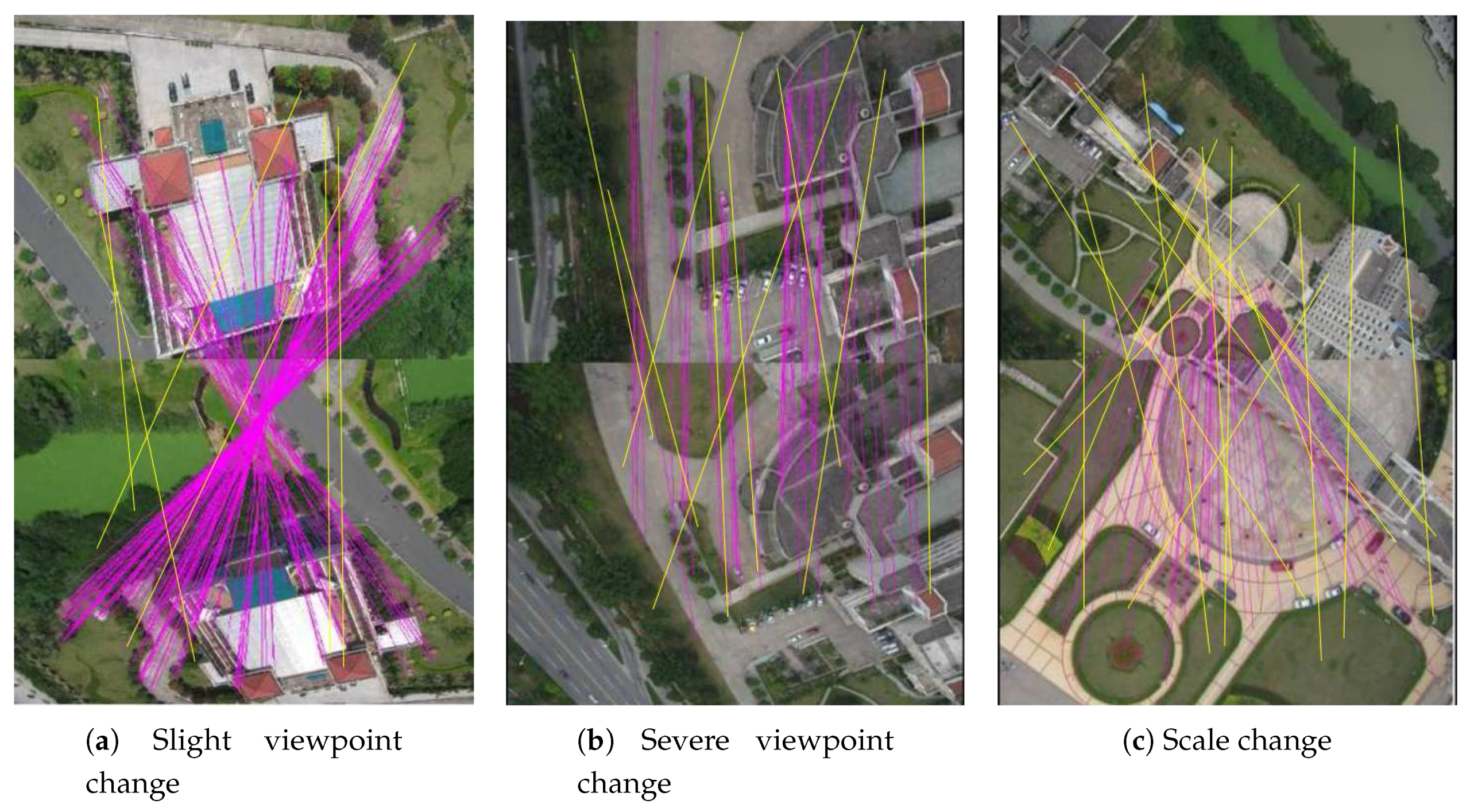
Transform estimation is an essential process in many remote sensing applications. For example, in the tasks of image or point cloud registration [1,2,3,4], change detection [5], large scale 3D reconstruction, and image stitching [6], data that acquired from different sensors, different time, and different angles should be transformed to a unified coordinate system. Therefore, the performance of these systems are rely on the accuracy of the estimated transformations. As for UAV aerial images, typical applications including large scale image stitching [7] and image-based 3D reconstruction [8]. The estimators are mainly based on matched keypoinits between UAV images. Mainstream feature descriptors such as Scale Invariant Feature Transform (SIFT) [9], Speeded Up Robust Features (SURF) [10], or binary descriptors [11] often couple with k-dimensional tree method [12] for feature matching. As shown in Figure 1a–c, SIFT descriptors have been extracted from two images of the same scene, respectively with severe viewpoint change, slight viewpoint change, and scale change. The matching results are represented by the lines among matched keypoints. Noteworthy that the pink lines depict the correct matched results, while the yellow lines represent the wrong matched keypoints. One can see that feature matching approach only consider the similarity between feature descriptor, while neglecting the consistency of the space distribution of matched feature points. As a consequent, the wrong matches may influence the accuracy of camera poses, which are derived from the estimated transformations. Therefore, we need to remove the wrong matches while keeping the correct matches as many as possible. This process is called matched feature refinement, where the correct and the wrong matches are denoted as inliers and outliers, respectively.
As for the transform estimation algorithm, Random Sample Consensus (RANSAC) [13] is one of the most famous that has been widely used in remote sensing area, such as registration [14], robot localization [15] and plane fitting in point clouds [16]. Typically, RANSAC for UAV-based image transform estimation algorithm includes the following three key steps. First, one need to choose an appropriate model/structure, usually fundamental or homographic matrix, to represent the transform between two UAV images. Second, a sample subset contains minimal data items is randomly selected from the matched keypoints. Then a fitting transform and the corresponding parameters are computed using only the elements of this sample subset. Third, check the consistency of the entire matched keypoints according to the transformation which is obtained from the second step. A matched feature pair will be considered as an outlier if the fitting residual exceeds a specified threshold. Otherwise, the matched pair will be regarded as an inlier.
Although RANSAC is an efficient tool for generating candidate transform, the success of hypothesise-and-verify scheme relies on “hitting” at least one minimal subset containing only inliers of a particular genuine instance of the geometric model. Under RANSAC, each member of a subset S is chosen randomly without replacement. Assume that the size of a minimal subset is p, the number of all matched feature pairs is denoted as N with . Then the probability that S contains all inliers is approximately , where is the outlier rate. Note that decreases exponentially with p. In the case of UAV aerial images transform estimation, we have for homographies and or for fundamental matrices. Since large scale scene usually consists of several planes, the pseudo outliers rate is very high in this situation. Namely the value of may be close to 1, where the probability of S contains all inliers is drastically decreased.
It is worth noting that matched keypoints in UAV aerial images are usually contaminated with heavy wrong matches due to the complex depth of field, repetitive pattern, etc. In other words, for large value of p, consecutively getting p inliers via pure random selection is not an easy task. Thanks to the widespread usage of robust estimators in computer vision, many innovations have been proposed to speed-up random hypothesis generation. These methods aim to guide the sampling process such that the probability of hitting an all-inlier subset is improved. The trick is to endow each input features with a prior probability of being an inlier. Consequently, that data with high probabilities are more likely to be simultaneously selected. For example, Chin [17] proposed a guided sampling scheme, called Mult-GS, which is driven only by residual sorting information and does not require domain-specific knowledge. Multi-GS uses feature similarity within a fixed residual window to evaluate whether two keypoints pair come from the same transform or not. However, experimental results show that setting fixed residual window size may reduce the robustness of the sampling process, since the performances are sensitive to the size of the residual window.
In order to solve this problem, we proposed more flexible strategies to determine the window size. The inlier probabilities are conditioned on the selected feature pairs and the similarity enables accurate hypothesis sampling. First, a relaxation residual window size is employed for evaluating the highest similarity within a relaxation model length. Second, we fixed the number of overlap structures with sliding the window size for computing the similarity. Third, a similarity metric that based on the permutation of residual values is proposed. The metric not only includes the number of overlap structures, but also gives penalty to the number of reverse order within the overlap structures.The experimental results conducted on our UAV remote sensing images show that the proposed three algorithms are all superior to Multi-GS in the condition of severe perspective distortion due to viewpoint change.
2. Related Works
The simplest strategy for estimating transformation between matched features is to minimize the square of transformed residuals of keypoints. There are many variants of this scheme, such as Weighted Least Squares (WLS) [18], M estimator [19], Least Median of Squares (LMS) [20], S estimator [21], Repeated Median Mstimator [22]. Although simple and fast, the break point of these methods are normally higher than , since the performance is sensitive to the percentage of outliers. The mainstream approaches are mostly based on hypothesis-and-verify strategy. Specially, many enhancements on the hypothesis-and-verify framework are proposed in the framework of RANSAC. For example, Progressive Sample Consensus(PROSAC) [23] employs the most promising keypoint correspondences to generate hypotheses. Although consistent, PROSAC may fail in repetitive texture regions where the feature descriptor are usually not distinguish. Other works include Optimal Randomized RANSAC [24], Adaptive Scale Kernel Consensus (ASKC) [25] and Iterative Kth Ordered Scale Estimator (IKOSE) [26], etc. In order to improve the accuracy of transformation between oblique aerial image, Hu et al. [27] proposed a spatial relationship scheme that employed angular, location and neighbor constraint to remove outliers. However, these methods cannot guarantee the consistency of hypotheses due to their randomized nature.
Recently, some guided sampling methods have been proposed for accelerating the hypothesis generation. This strategy usually has a process of feature pairs similarity analysis in the sampling stage, which are mainly based on feature matching scores or location residuals. Typical methods including dynamic and hierarchical algorithm [28], Top-k [29], Global optimization [30], Multi-GS [17], kernal-based method [31], and Random Cluster Model Sampling (RCMSA) [32,33], etc. Specially, Multi-GS accelerates hypothesis sampling by guiding it with information derived from residual sorting. It is crucial that sorted residual sequence encodes the probability of two points come from the same model, which encourages sampling within coherent structures and thus can rapidly generate all-inlier minimal subsets. As for RCMSA [32,33], its basic idea is to enhance the robustness of minimal subset. As a result, they used feature clusters for generating candidate structures. Moreover, the mode seeking approach [34] employed Medoid Shift [35] for seeking the mode in residual sorts. The candidate structures then can be generated via the conditional probability that based on each mode. Similarly, Residual Consensus(RECON) [36] used Kolmogorov-Smirnov (KS) [37] test to evaluate whether two residual sort come from the same distribution or not. Then the sampling process is based on the score of KS test. On the other hand, in [38,39,40], information exploited from keypoint matching scores is used to extract promising hypothesis. Unfortunately, for multi-structure data, these methods usually fail to achieve one clean solution within a reasonable time budget. Note that all of Multi-GS [17], RCMSA [32,33] and Multi-GS-Oset [41] accelerate promising hypothesis generation by using information derived from residual sorting. These methods can effectively handle most multi-structure data. However, the limitation is that they assume spatial smoothness (i.e., the inliers of a model instance must be coherent). This assumption is more restrictive than the spatial proximity assumed by [42] and is often violated in practice.
We are also aware of recent work proposed in [43], which guides sampling process by using residual information as well. This method performs a sequential “fit-and-remove” procedure to estimate model instances of multi-structure data. Similarly, Lai [44] proposed the Efficient Guided Hypothesis Generation (EGHG) method for multi-structure epipolar geometry estimation. This algorithm combines two guided sampling strategies: a global and a local sampling strategy, which are all guided by using both spatial sampling probabilities and keypoint matching scores, for efficiently achieves accurate solutions. Noteworthy that these transform estimators has been successfully used in many remote sensing tasks, such as fundamental matrix estimation with only translation and radial distortion [45], multi-modal correspondence [46], Quasi-Homography transform estimation for wide baseline stereo [47], and rotation-scaling-translation estimation based on fractal image model [48]. In particular, robust estimators are suitable for the model fitting task in point clouds, such as plane and roof reconstruction [49,50,51], road fitting and segmentation [52,53], etc. Apart from the “fit-and-remove” scheme, there are several strategies for estimating transformation. For example, Zai et al. [54] proposed a covariance matrix descriptors to find candidate correspondences. Then a non-cooperative game is constructed to isolate mutual compatible correspondences, which are considered as true positives. As a consequent, the transformation can be acquired via correct correspondences. Although these methods have achieved promising performances in many applications, estimating the transformation between UAV images is still a challenging task, due to severe viewpoint changes, repetitive pattern and complex depth of field.
3. The Proposed Residual Analysis Method
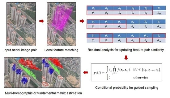
Pipeline of the proposed sampling algorithm including three key steps, which are respectively match, sample and update. In the match stage, feature extraction and matching, such as PSIFT [55] along with kd-tree, are conducted on two UAV aerial images. Parallax of the two images should larger than a certain threshold to ensure that keypoint coordinates in two images are not identical. In the sampling stage, the candidate models are generated from minimum feature sets. Entry in each set is sampled based on conditional probability distribution, which is related to the similarity among keypoint pairs. In the updating stage, similarity matrix is updated via the overlap structures in sorted residual sequence. The conditional probability distribution is then updated from the similarity matrix. Details are given as follows.
3.1. Similarity Evaluation Based on the Distribution of Structures
As mentioned in the pipeline, similarity between matched keypoint pairs play an important role in the sampling process. Therefore, this section proposes three metrics for evaluating the similarity. Let denotes an input matched keypoint set between two UAV aerial images, where stands for the i-th matched pair. Without loss of generality, let , where and are the coordinates of matched feature points, respectively. Let denote M transform matrices, then the residuals for are calculated via the feature coordinate transformation. Assume that the residuals of the i-th matched keypoint pair are the following equation.
where denotes the m-th residual for the i-th matched keypoint pair. Since the similarity is based on residual order, we then sort the sequence according to the residual values, given as follows.
where represents the m-th smallest residual. For example, stands for the best transformation of the i-th matched keypoint pair. Based on the residual order, Multi-GS proposed a similarity metric that relates to the number of overlapping within top h structures, as given in Equation (3).
where denotes the number of overlap structures in top h structures for matched keypoint pair and , concerning with . Multi-GS recommended the length of residual window size as . However, our experiments reveal that there exists two key factors in the sampling process. First, the size of residual window is very important in generating promising models. In other words, the window size should be adaptive determined by the distribution of residuals. Second, mainstream methods didn’t take the order of residual into account, which may results in different order with the same similarity. In order to handle these two problems, we proposed two flexible strategies, terms in relaxation window and sliding model, for adaptively select the window size. Moreover, we investigate the influence of residual order, then employ a penalty term in the similarity metric to enhance the robustness of sampling process.
3.1.1. Relaxation Windows
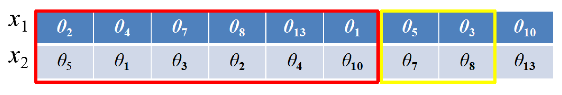
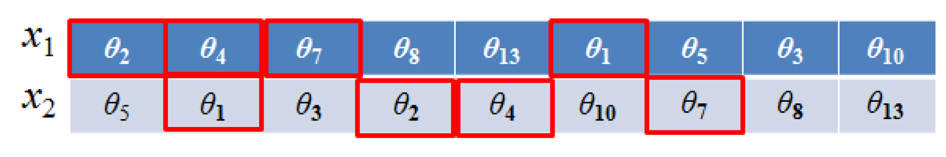
Figure 2 depicts the motivation of the proposed relaxation method. For example, assume are M transform matrices or candidate structures, then two residual sequences can be generated from matched keypoint pairs of and , respectively. Let the window size in residual sequences is equal to 6 (red rectangle). Note that there are three overlapping models, namely , , , within the specific window. As a consequent, in Multi-GS, the similarity between matched keypoint pair and is equal to , which is the proportion of overlapping models within the window. It is worth noting that if the window size is extended to 9, we then have . As mentioned above, this phenomenon is caused by the setting of fixed window size. Therefore, we introduce a relaxation strategy for generating an appropriate size of window. The motivation is to evaluate the similarity from more windows, then the results may objectively recover the possibility of whether two pairs of matched features are come from the same structure or not. The details of our relaxation method is given as the following equation:
where denotes the number of overlap structures in top h structures for matched keypoint pair and , concerning with , and h denotes the baseline window size, stands for the relaxation area. Then the the relaxation strategy searching for the maximum similarity from . For example, in Figure 2, given with (yellow rectangle), we need to search the maximum similarity with the window size that ranges from 6 to 8. As a consequent, the similarity value would be , since the similarity will reach the maximum value when the window size is 8. In this case, the overlap models within the window are .
Specially, our experimental results show that , will obtain more promising results, which means the searching interval is . The details of parameter selection are shown in the experimental results session.
3.1.2. Sliding Windows
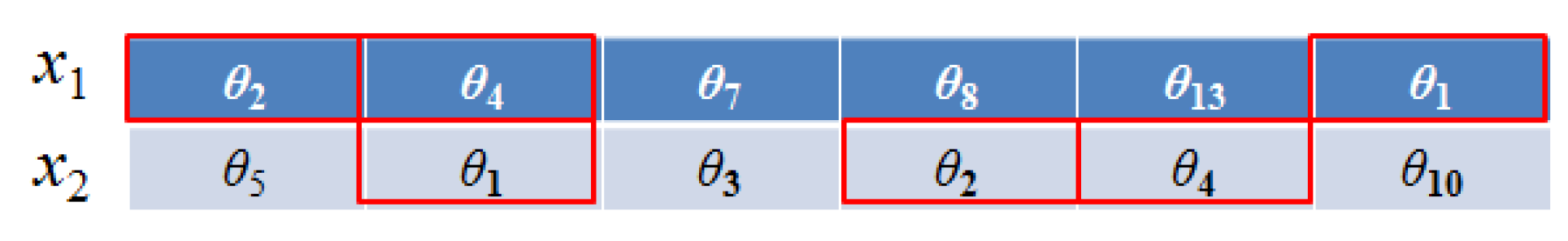
An alternative approach to evaluate the similarity is to fix the number of overlap hypothesises, while varying the window length to search an appropriate similarity. The basic idea is to calculate the number of overlap structures in spanning windows, until the number of the overlap structures meet a specified parameter. Then the similarity is derived from the proportion of the fix number and the searching length. The equation is given as below:
where is the fixed number of models, K denotes the length of search window with . From the section of experiment results, we found that balance the trade-off between time complexity and sampling accuracy. Figure 3 gives an example of the proposed sliding approach. Assume that , we then have when . As a consequent, is the similarity between matched feature pair and .
3.1.3. Feature Similarity Based on Reverse Residual Order
As mentioned above, Multi-GS only consider the number of overlap hypothesises within a fixed window, while neglecting the fact that residual order is very important for feature similarity evaluation. To this end, we propose a similarity metric that based on the permutation of residual values. The similarity equation is given as follows:
while is a penalty factor relating to the window length h, denotes the reverse number of the overlap structures within a specific window.
Figure 4 gives an example of the proposed metric. Let the window length , the normalized factor . Note that the overlap model set of is , while for . Let be the baseline order, then and are the reverse pairs in the sorted residual sequence of . As a consequent, the reverse number is equal to 2, and then the similarity between and is . Since the number of reverse order is associated with h, in order to guarantee , we then set with .
3.2. Candidate Structure Sampling Based on Conditional Probability Distribution
The similarity between matched keypoint pairs reflects the possibility of whether the keypoints are from the same structure. Then the similarity should be with smaller value between different structure, while with higher value within the same structure. In other words, the similarity can be seen as the probability to sample candidate structures. Namely, the matched feature pairs are sampled according to a conditional probability.
Let , where denotes the minimal number of matched keypoint pairs that can be used to generate a candidate hypothesis. First, randomly sample a matched pair , then the second matched pair is generated in a greedy probability way based on the similarity with the first matched pair. The conditional probability is given as follows:
where is the normalize factor. Obviously, the higher value of means the higher probability that a matched pair may be chosen. The rest matched pairs can be selected in the same manner. Assume that the selection of each pair is independently, then the probability of the -th matched keypoint pair can be expressed as the product of the probability that related to k matched pairs, which have already been selected. The equation is given as follows:
Therefore, candidate transformations are sampled based on the distribution of conditional probability. Once a new hypothesis/transformation is generated, it can be added to the structure set . Meanwhile, the similarity matrix between matched keypoint pairs can be updated according to residuals generated via the new hypothesis. Since the similarity values are based on residual analysis, the computational cost for updating the similarity matrix is really expensive. In order to speed up the sampling process, the similarity matrix can be updated after sampling a patch of structures. In other words, once a new candidate structure is generated, it may not been inserted to the structure set immediately. For example, the similarity matrix can be updated after candidate structures are generated, where the residual list for each matched pair is updated via binary insert algorithm.
4. Algorithm Summary
As mentioned before, the proposed approach aims at extracting fundamental matrix and multi-homographic transformations between high resolution UAV aerial images from different viewpoints. Algorithm 1 presents the pipeline of the proposed strategy, where the fundamental and the homographic matrices need 4, 8 matched keypoint pairs, respectively.
| Algorithm 1 Transformation Estimation Based on Residual Analysis. |
| Input: Matched keypoint set P of input images and ; |
| Initialize: Sampling threshold t; Scale of inliers s. |
| Output: Fundamental matrix and homographic matrices between and . |
| Inliers and the outliers of P. |
|
5. Time Complexity Analysis
Since the proposed three strategies are motivated by Multi-GS, we will then analyze the time complexity comparison among Multi-GS and the proposed methods. Note that for each iteration, the following two steps of Multi-GS are time-consuming. First, hypothesises are generated based on conditional probability, which are related to the similarity matrix for each feature pair. Second, once specific batch of transformations are generated, the total number of transformations in model set would be expanded and then the similarity matrix should be updated. Obviously, the cost of updating similarity matrix is far more higher than generating transformations. Therefore, the time complexity is mainly depended on how to generate effective structures based on similarity among feature pairs.
As mentioned before, let M, N denote the number of total transformations and matched features, respectively. h, k stand for the residual window length, and the number of overlap hypothesises/structures in the window. b denotes the number of structures in a batch. For one hand, the cost of updating residual order list for all matched features is . For another hand, the cost of updating the similarity between each matched pair is , given that the number of overlap transformations is linearly related to the window length. Since the number of transformations in a batch is far less the number of matched feature pairs, namely , then the total time complexity of Multi-GS for each iteration is .
It is worth noting that the proposed method including three strategies, which are respectively relaxation window, sliding window and reverse residual order. Since the total complexity of Multi-GS is rely on the process of updating similarity matrix, the comparison then focus on the similarity for each approach independently. Note that for the relaxation window, the window size ranges from to . Since we set in the section of experiments, the cost of updating similarity matrix is still . It means that the total time complexity of the proposed relaxation scheme is also .
The second scheme of this paper is sliding window, which calculates the number of overlap structures in spanning windows until the number of overlap structures or the length of window reach a specific parameter. Note that the searching length can be less than h, which means that the time complexity is no more than .
As for the reverse residual order approach, we need to calculate the reverse number in a specific residual window size. Obviously, the residual sorting process can be done within , where k denotes the number of overlap structures in the window. Since the reverse residual order follows by overlapping calculation, the time complexity is less than . Note that in the later stage of the algorithm, the number of overlap candidate models from different structure is very small. Then the the time complexity is about equal to , where C stands for the number of structures in the scene. For example, as for five structures task, we can set , , . Given two features from a same structure, we found that in the late stage of the algorithm. Therefore, the proportion between total cost of reverse order and multi-GS is . One can see that in the section of experimental results, the time cost comparison supports our analysis on the complexity.
6. Experiments
This section aims at evaluating the performance proposed sampling algorithm. Therefore, we compared the proposed strategies with RANSAC and Multi-GS, respectively with multi-homographic and fundamental matrix extraction, on the high-resolution aerial image dataset acquired from our UAV remote sensing systems. The image dataset contains all kinds of configurations including low-altitude buildings, skyscrapers areas and country scenes. A total of 12 pair of images were acquired under various conditions exhibiting different challenges such as scale changes, slight perspective distortion and severe perspective distortion. Specially, the size of each aerial image is 30 million pixels, where these images were taken at the height of about 400 meters. Concerning with the focus of our camera, each pixel represents 1 × 1 cm∼5 × 5 cm on the ground, which means the resolution surpass traditional remote sensing data, such as satellite images, SAR images, etc.
Moreover, in order to evaluate the efficiency of the proposed method, some metrics have been employed such as the number of valid structures in specific time, run time of the whole sampling process, and the mean errors of fundamental matrix which are calculated by all inliers. The results are compared to the ground truths that are acquired from hand-craft ground control points.
6.1. Parameters Setting
As mentioned before, the window size h is a key parameter for computing the similarity metric. Chin [2] recommended an appropriate value with . In the proposed strategies, we set in the relaxation method, where the relaxation factor . As for the sliding window approach, the number of overlap structures is set as . In order to give fair comparisons, the window length in residual reverse order is also as , while the penalty factor . As for the homographic transformation, the metrics for evaluation including the number of valid structures that generated within 10 s, and the run time (seconds) of hitting all structures of each methods. As for the fundamental matrix, we evaluate the mean square error of distance between epipolar line and the corresponding feature points.
6.2. The Estimation of Multi-Homographic Transformation
According to the principle of homographic transform, there may exist multiple homographic transformations in a scene with a number of planes, such as multi-depth of filed. It is worth noting that the process of mult-planes extraction is a key component in the task of aerial image stitching. For example, the accuracy of large scale orthophotomap depends on the stitching results. Therefore, this subsection aims at evaluating the efficiency multi-homograpihcs extraction of the proposed method on our low altitude remote sensing images. In order to give objective results, each algorithm runs 50 times and the average results are recorded. Experimental evaluations include the number of sampling structures, valid structures, and the run time of extracting all valid structures. In order to show the efficiency of our proposed method, from experiment 1 to experiment 3, we aim at evaluating the efficiency of multi-plane or multi-depth of filed extraction from UAV aerial images. Therefore, three typical aerial images with slight viewpoint changes and severe viewpoint changes have been selected to test our proposed schemes.
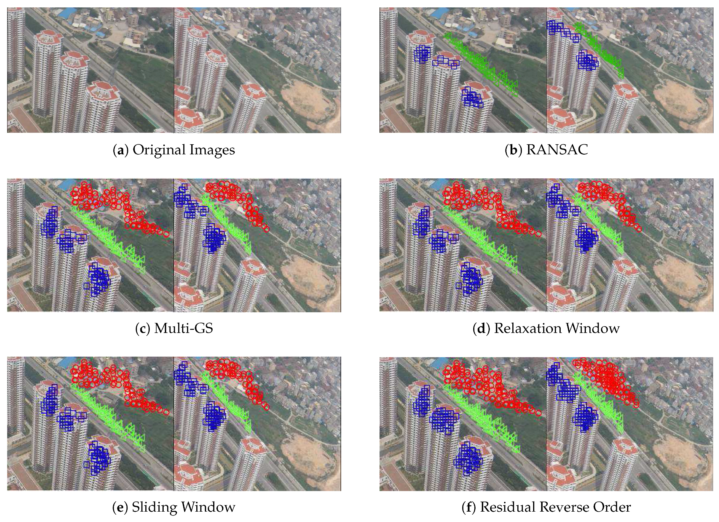
6.2.1. Experiment 1: Three Structures in Low-Altitude Aerial Images with Slight Viewpoint Change
This experiment aims at measuring the robustness to slight perspective distortion caused by viewpoint and camera orientation changes with the presence of tall buildings. As shown in Figure 5a, Apartments 1 contains high-rise buildings seen from different view-points. Note that the viewpoint shift induces a slight perspective deformation on the building and the surrounding landscape. As a result, the matched features on the roof of the high-rise buildings, the road, and the low-rise buildings are with different depth of field. Namely, these matched features can be expressed via different homographic transformations. Results for all five algorithms are presented in Figure 5b–f. Firstly, RANSAC failed in extracting all valid structure within 10 s. Secondly, the relaxation and the sliding window method generated almost the same inliers with Multi-GS algorithm. Last but not the least, the reverse residual order method achieved the best performance, concerning with the number of the correct matches that have been preserved. Part of the explanation is the height of the buildings which creates noticeable planes for which methods have a hard time to deal with. This illustrates the advantage of guided sampling approaches which incorporates a sampling prior within its definition.
6.2.2. Experiment 2: Five Structures in Low-Altitude Aerial Images with Severe Viewpoint Change
In this experiment, a pair of high resolution aerial images (HQU) with five structures has been acquired from distinctive different viewpoints. These images show buildings captured from different view-points and which suffer severe deformation compared to the previous scenarios.
As shown in Figure 6a, since HQU were acquired from a low-altitude camera pointing towards the high-rise building, the scene contains severe perspective distortion. The feature matching results, which including inliers and outliers, together with hand-craft control points are regarded as the input matched points. Note there are five homographic transformations in this image pair due to the complex depth of filed, which are respectively represented as green triangle, blue square, red circle, yellow diamond, light blue diamond. Figure 6b–f shows sampling results for RANSAC, Multi-GS, relaxation window, sliding window, and reverse residual order, respectively. Note that RANSAC only found out two valid homographic transformations, since the ratio of outlier and pseudo outlier is pretty low. This phenomenon reveals that blind searching strategy does’t achieve promising results in complex depth of filed or there are multi-planes in the scene. It is worth noting that in the case of yellow diamond, only reverse residual order-based sampling strategy extract the valid structure within the specific time. Part of the explanation is the inlier rate of this structure is very low. In addition, the coordinates of feature points in this structure/plane are close to that of red circle. Namely, the feature points in yellow diamond may influence the performance of all algorithms. This phenomenon reveals that reverse residual order is an efficient scheme to evaluate the probability of two feature pair come from the same structure.
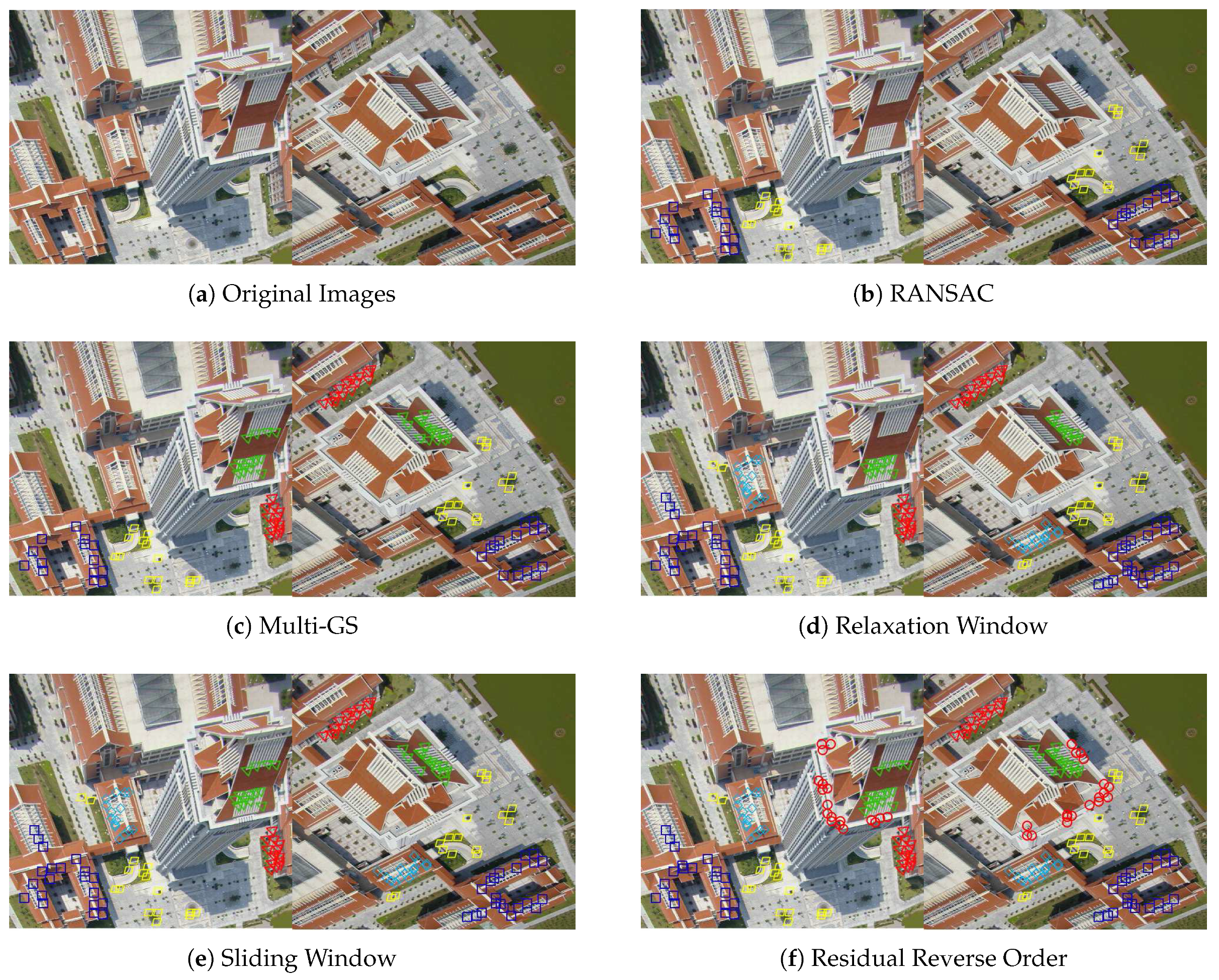
6.2.3. Experiment 3: Six Structures in Low-Altitude Aerial Images with Severe Viewpoint Change
In this experiment, a pair of high resolution aerial images (Library) with six structures has been acquired from distinctive different viewpoints, which suffering severe deformation compared to the previous scenarios. Figure 7a shows that there exists multi-planes and repetitive patterns/features in the scene, since the camera is much closer to the roof of the building than the street level. From Figure 7b–f, one can see the sampling results for RANSAC, Multi-GS, relaxation window, sliding model, and reverse residual order, respectively. Where the six structures are represented as green triangle, blue square, red circle, yellow diamond, light blue diamond, and red triangle, respectively. As for RANSAC, we can draw the same conclusions as we did in experiment 5, since RANSAC doesn’t extract all transformations due to the high percentage of wrong matches and pseudo outlier. One can see that even guided sampling methods such as Multi-GS, relaxation window and sliding model miss the structure of red circle, where the features are distributed around the roof of the high-rise building. In this case, reverse order of residuals approach was the only one to find out all homographic transformations. This fact clearly underlines the advantage of the proposed method, which is robust to all kinds of scenes including large viewpoint change and repetitive patterns that may induce complex multi-structure problem.
6.2.4. Experiment 4: Comparisons of Sampling Structures and Running Time on Low-Altitude Aerial Images
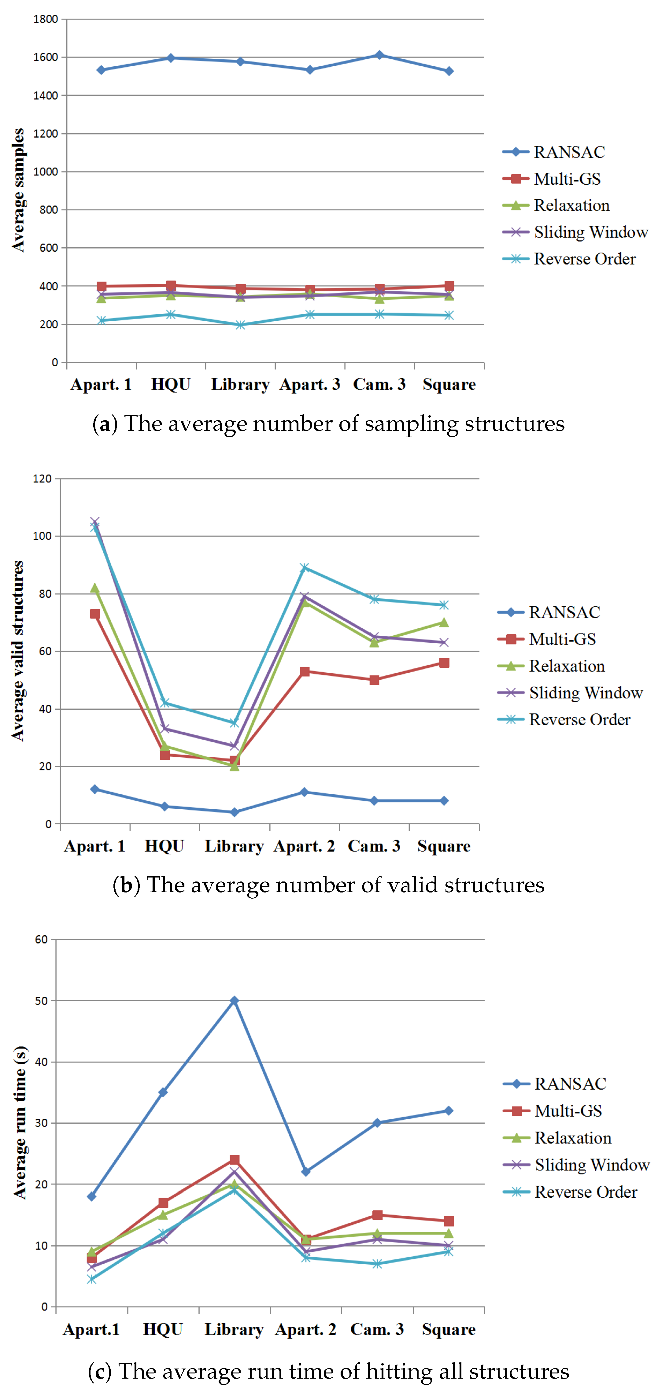
Figure 8 shows the average number of sampling structures, the average number of valid structures, and the run time (seconds) of hitting all structures on our UAV remote sensing dataset including Apartments 1, HQU, Library, Apartments 2, Campus 3, and Square, respectively with 3, 5, 6, 3, 4, 4 structures. Specially, each image pair has different outliers/false matched feature rate. Overall, the reverse residual order scheme needs analyzing the number of reverse order within a specific window, which results in increasing the time complexity in the early stage of sampling process. However, the feature similarity prevents high overlap structures with high reverse order in the late stage of the algorithm. It might be objective to say that the similarity of reverse residual order reflects the probability of whether two features are come from same structure. In most case, reverse residual order-based guide sampling algorithm is the fastest as for extracting all valid structures.
6.3. Experiment 5: Accuracy of Fundamental Matrix
In this section, we show that the fundamental matrix generated via our algorithms are globally more accurate than that of the RANSAC and Multi-GS. We do so by calculating the average alignment error for each method according to its fundamental matrix F. A fundamental matrix is a matrix which converts a point p in one image into an epipolar line in the second image. Since the matching point q in the second image should always lies on that epipolar line, the distance between q and should be zero. Therefore, the validation procedure goes as follows:
- Manually select 30 match points for each aerial image. These matches are called “ground truth matches” (GT-M).
- For each image pair and each method, get inter-image matches and compute the fundamental matrix accordingly.
- Given the GT-M of an image pair, compute the average Euclidian error for each method. For example, given 2 GT-M points p and q and the fundamental matrix of method i, compute the epipolar line of p and get the Euclidian error between and q. In that case, a good evaluating method should have a small error.
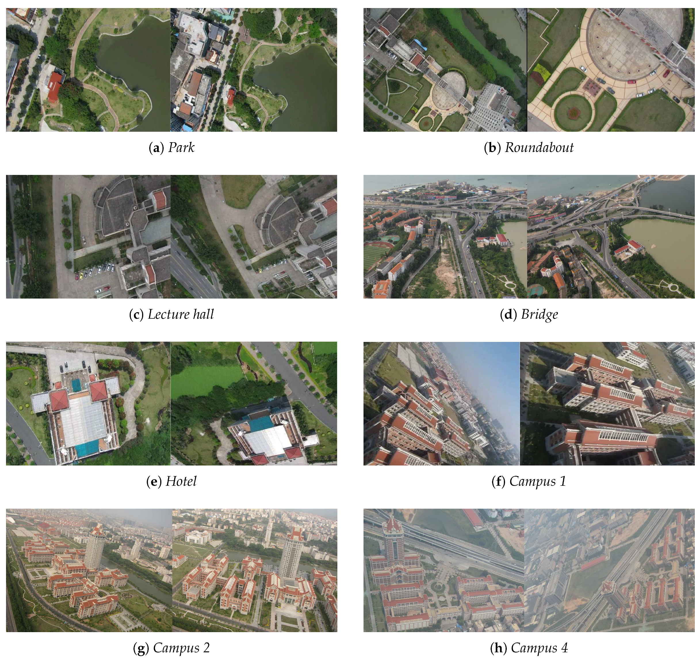
As shown in Figure 9, we select 8 image pairs from our aerial dataset, respectively in the category of “Scale Change”, “Slight Viewpoint Change”, and “Severe Viewpoint Change” , to evaluate the efficiency of the proposed schemes. Note that Apartment 1 is also included in category of “Slight Viewpoint Change”. Table 1 contains the average error for 9 aerial images. As can be seen in the table, for each method, complex scenes with severe perspective distortion induce larger average error. Also the reader shall notice that guide sampling based methods achieved higher accuracy than RANSAC except Square. Specifically, In the set of severe viewpoint change, the guide sampling methods outperform significantly than RANSAC, since the depth of filed is also complex than scale change and slight viewpoint change dataset. This fact reveals that guide sampling strategy is suitable for complex scene, which may increase the accuracy of camera pose. Moreover, one can see that the four guide sampling methods have not much differences in the dataset of scale change. While in the viewpoint change datasets, the reverse residual order method achieved the best performance than other methods, which means that more feature matching pairs result in more probability of generating good transformation.
Moreover, we evaluate the efficiency of RRO+SO and RRO+SW in fundamental matrix extraction. Table 1 shows that the performance of RRO+SO and RRO+SW are worse than RRO, SO, or SW in the case of easy tasks such as scale change. The main reason is that the number of sampled hypothesis per second may decreased, since RRO should performed after SO or SW, which increase the time complexity of updating similarity matrix. However, in complex scenes such as severe viewpoint change, RRO+SO and RRO+SW achieved comparable or even better results than RRO. This phenomenon reveals that the combinations of RRO+SO and RRO+SW are suitable to high outlier or pseudo outlier rate scenes.
6.4. Algorithm Discussion
Based on the five experimental results mentioned above, here we make a detailed analysis and comparisons on the advantages and the disadvantages of Relational Window (RW), Sliding Window (SW), Reverse Residual Order (RRO).
RW employs a relaxation interval to evaluate the similarity between matched feature pairs in order to handle the boundary effect in fixed-size window scheme. Experimental results show that relaxation window scheme achieved better performance than fixed-size window under the same time complexity. Disadvantages of RW are: (1) The size of relaxation window is a hyper-parameter, which is determined empirically; (2) The residual order was not taken into account.
SW fixes the number of overlap structure/hypothesis while varying the window length to compute the similarity. SW can find out the number of overlap structures in spanning windows, which provides more flexible scheme of the window size selection. Disadvantages of SW are: (1) The time complexity may increase when dealing with low similarity feature pair; (2) The residual order was not taken into account.
RRO provides a probability framework to determine whether two feature pair come from a same structure by analyzing the difference of residual order among each feature pair. Experimental results showed that RRO achieved best performance in complex scene with five or six structures. Disadvantages of RRO are (1) The computation of reverse number is time-consuming; (2) It may not work well on easy tasks, such as there are only one structure or two structures in the scene.
7. Conclusions
Evaluating the transformation between two UAV aerial images acquired from the same scene is a fundamental step of camera pose estimation and UAV image-based applications, such as stitching and 3D reconstruction. In this paper, we presented three schemes for estimating the transformation between different viewpoint of UAV remote sensing images. Specifically, we analyzed the drawback of RANSAC with brutal sampling. Moreover, state-of-the-art method such as Multi-GS suffers from fixed residual window size and unable to deal with the order of structures within a window. To this end, we proposed three strategies for evaluating transformation between UAV images. Firstly, a relaxation window size is employed for evaluating the similarity between feature pairs. The basic idea is to acquire the highest similarity within a relaxation model length, which has been proved to be unsensitive to the window size. Secondly, we fixed the number of overlap structures, while the window size can be flexible to evaluate the similarity. Thirdly, we found that Multi-GS only consider the number of overlap structures within a window, while neglecting the fact that residual order for feature similarity evaluation. Therefore, we propose a similarity metric that is based on the permutation of residual values. The metric not only includes the number of overlap structures, but also gives punishment to number of reverse order within the overlap structures. The experimental results conducted on UAV remote sensing images show that the proposed three schemes and Multi-GS perform equally well on images with scale change, while the proposed sample scheme performs better in the presence of severe perspective distortion and multi-structures, respectively due to viewpoint change and complex depth of field. Future research will aim at reducing the complexity of reverse residual order.
Acknowledgments
This work is supported by the National Natural Science Foundation of China under Grant No. 61363049, No. 61702251, No. 61572409, No. 61402386 and No. 61571188, the Key Technical Project of Fujian Province under Grant No. 2017H6015, the Natural Science Foundation of Fujian Province under Grant Nos. 2016J01310 and 2016J01309, the Open Project Program of the Key Laboratory of Nondestructive Testing, Ministry of Education under Grant No. ZD201429007. Fujian Province 2011 Collaborative Innovation Center of TCM Health Management and Collaborative Innovation Center of Chinese Oolong Tea Industry-Collaborative Innovation Center (2011) of Fujian Province.
Author Contributions
Guorong Cai designed the algorithm, conducted experiments, and led the writing of the manuscript. Songzhi Su managed the project, conceived the experiments, and assisted in writing the manuscript. Chengcai Leng designed and conducted experiments, and assisted in writing the manuscript. Yundong Wu performed the experiments, collected and analyzed the UAV aerial image dataset. Feng Lu took part in designing experiments, and assisted in writing the manuscript.
Conflicts of Interest
The authors declare no conflict of interest.
References
- Yang, K.; Pan, A.; Yang, Y.; Zhang, S.; Ong, S.H.; Tang, H. Remote Sensing Image Registration Using Multiple Image Features. Remote Sens. 2017, 9, 581. [Google Scholar] [CrossRef]
- Yang, B.; Chen, C. Automatic registration of UAV-borne sequent images and LiDAR data. ISPRS J. Photogramm. Remote Sens. 2015, 101, 262–274. [Google Scholar] [CrossRef]
- Liu, S.; Tong, X.; Chen, J.; Liu, X.; Sun, W.; Xie, H.; Chen, P.; Jin, Y.; Ye, Z. A Linear Feature-Based Approach for the Registration of Unmanned Aerial Vehicle Remotely-Sensed Images and Airborne LiDAR Data. Remote Sens. 2016, 8, 82. [Google Scholar] [CrossRef]
- Yang, B.; Zang, Y.; Dong, Z.; Huanga, R. An automated method to register airborne and terrestrial laser scanning point clouds. ISPRS J. Photogramm. Remote Sens. 2015, 109, 62–76. [Google Scholar] [CrossRef]
- Li, W.; Sun, K.; Li, D.; Bai, T.; Sui, H. A New Approach to Performing Bundle Adjustment for Time Series UAV Images 3D Building Change Detection. Remote Sens. 2017, 9, 625. [Google Scholar] [CrossRef]
- Liu, J.; Gong, J.; Guo, B.; Zhang, W. A Novel Adjustment Model for Mosaicking Low-Overlap Sweeping Images. IEEE Trans. Geosci. Remote Sens. 2017, in press. [Google Scholar] [CrossRef]
- Xu, Y.; Ou, J.; He, H.; Zhang, X.; Mills, J. Mosaicking of Unmanned Aerial Vehicle Imagery in the Absence of Camera Poses. Remote Sens. 2016, 8, 204. [Google Scholar] [CrossRef]
- Xu, Z.; Wu, L.; Gerke, M.; Wang, R.; Yang, H. Skeletal camera network embedded structure-from-motion for 3D scene reconstruction from UAV images. ISPRS J. Photogramm. Remote Sens. 2016, 121, 113–127. [Google Scholar] [CrossRef]
- Lowe, D. Distinctive image features from scale-invariant keypoints. Int. J. Comput. Vis. 2004, 60, 91–110. [Google Scholar] [CrossRef]
- Bay, H.; Ess, A.; Tuytelaars, T.; Van Gool, L. Speeded-Up Robust Features (SURF). Comput. Vis. Image Underst. 2008, 110, 346–359. [Google Scholar] [CrossRef]
- Rublee, E.; Rabaud, V.; Konolige, K.; et al. ORB: An efficient alternative to SIFT or SURF. In Proceedings of the 2011 IEEE International Conference on Computer Vision (ICCV), Barcelona, Spain, 6–13 November 2011; pp. 2564–2571. [Google Scholar]
- Bentley, J. Multidimensional binary search trees used for associative searching. Commun. ACM 1975, 18, 509–517. [Google Scholar] [CrossRef]
- Fischler, M.A.; Bolles, R.C. Random sample consensus: A paradigm for model fitting with applications to image analysis and automated cartography. Commun. ACM 1981, 24, 381–395. [Google Scholar] [CrossRef]
- Zheng, L.; Yu, M.; Song, M.; Stefanidis, A.; Ji, Z.; Yang, C. Registration of Long-Strip Terrestrial Laser Scanning Point Clouds Using RANSAC and Closed Constraint Adjustment. Remote Sens. 2016, 8, 278. [Google Scholar] [CrossRef]
- Liu, Y.; Gu, Y.; Li, J.; Zhang, X. Robust Stereo Visual Odometry Using Improved RANSAC-Based Methods for Mobile Robot Localization. Sensors 2017, 17, 2339. [Google Scholar] [CrossRef] [PubMed]
- Li, L.; Yang, F.; Zhu, H.; Li, D.; Li, Y.; Tang, L. An Improved RANSAC for 3D Point Cloud Plane Segmentation Based on Normal Distribution Transformation Cells. Remote Sens. 2017, 9, 433. [Google Scholar] [CrossRef]
- Chin, T.J.; Yu, J.; Suter, D. Accelerated hypothesis generation for multi-structure data via preference analysis. IEEE Trans. Pattern Anal. Mach. Intell. 2012, 34, 625–638. [Google Scholar] [CrossRef] [PubMed]
- McElroy, F.W. A necessary and sufficient condition that ordinary least-squares estimators be best linear unbiased. J. Am. Stat. Assoc. 1967, 62, 1302–1304. [Google Scholar] [CrossRef]
- Huber, P.J. Robust Statistics; Springer: Berlin/Heidelberg, Germany, 1981. [Google Scholar]
- Rousseeuw, P.J. Least median of squares regression. J. Am. Stat. Assoc. 1984, 79, 871–880. [Google Scholar] [CrossRef]
- Rousseeuw, P.; Yohai, V. Robust regression by means of S-estimators. In Lecture Notes in Statistics; Springer: New York, NY, USA, 1984; Volume 26, pp. 256–272. [Google Scholar]
- Siegel, A.F. Robust regression using repeated medians. Biometrika 1982, 69, 242–244. [Google Scholar] [CrossRef]
- Chum, O.; Matas, J. Matching with PROSAC-Progressive Sample Consensus. In Proceedings of the IEEE Computer Society Conference on Computer Vision and Pattern Recognition (CVPR 2005), San Diego, CA, USA, 20–25 June 2005; pp. 220–226. [Google Scholar]
- Chum, O.; Matas, J. Optimal randomized RANSAC. IEEE Trans. Pattern Anal. Mach. Intell. 2008, 30, 1472–1482. [Google Scholar] [CrossRef] [PubMed]
- Wang, H.; Mirota, D.; Ishii, M.; Hager, G.D. Robust motion estimation and structure recovery from endoscopic image sequences with an adaptive scale kernel consensus estimator. In Proceedings of the IEEE Conference on Computer Vision and Pattern Recognition, Anchorage, AK, USA, 23–28 June 2008; pp. 1–7. [Google Scholar]
- Wang, H.; Chin, T.J.; Suter, D. Simultaneously fitting and segmenting multiple-structure data with outliers. IEEE Trans. Pattern Anal. Mach. Intell. 2012, 34, 1177–1192. [Google Scholar] [CrossRef] [PubMed]
- Hu, H.; Zhu, Q.; Du, Z.; Zhang, Y.; Ding, Y. A reliable feature point matching method for oblique aerial images using the spatial relationships of the point correspondences to remove outliers. Photogramm. Eng. Remote Sens. 2015, 81, 49–58. [Google Scholar] [CrossRef]
- Wong, H.S.; Chin, T.J.; Yu, J.; Suter, D. Dynamic and hierarchical multi-structure geometric model fitting. In Proceedings of the 2011 IEEE International Conference on Computer Vision (ICCV), Barcelona, Spain, 6–13 November 2011; pp. 1044–1051. [Google Scholar]
- Wong, H.S.; Chin, T.J.; Yu, J.; Suter, D. Effcient multi-dtructure robust fitting with incremental top-k lists comparison. In Proceedings of the 10th Asian Conference on Computer Vision, Queenstown, New Zealand, 8–12 November 2010; pp. 553–564. [Google Scholar]
- Yu, J.; Chin, T.J.; Suter, D. A global optimization approach to robust multi-model fitting. In Proceedings of the IEEE Conference on Computer Vision and Pattern Recognition, Colorado Springs, CO, USA, 20–25 June 2011; pp. 2041–2048. [Google Scholar]
- Chin, T.J.; Suter, D.; Wang, H. Multi-structure model selection via kernel optimization. In Proceedings of the IEEE Conference on Computer Vision and Pattern Recognition, San Francisco, CA, USA, 13–18 June 2010; pp. 3586–3593. [Google Scholar]
- Pham, T.; Chin, T.; Yu, J.; Suter, D. The random cluster model for robust geometric fitting. In Proceedings of the IEEE International Conference on Computer Vision and Pattern Recognition, Providence, RI, USA, 16–21 June 2012; pp. 710–717. [Google Scholar]
- Pham, T.T.; Chin, T.J.; Yu, J.; Suter, D. The random cluster model for robust geometric fitting. IEEE Trans. Pattern Anal. Mach. Intell. 2014, 36, 1658–1671. [Google Scholar] [CrossRef] [PubMed]
- Wong, H.S.; Chin, T.J.; Yu, J.; Suter, D. Mode seeking over permutations for rapid geometric model fitting. Pattern Recognit. 2013, 46, 257–271. [Google Scholar] [CrossRef]
- Sheikh, Y.A.; Khan, E.A.; Kanade, T. Mode-seeking by Medoidshifts. In Proceedings of the IEEE International Conference on Computer Vision and Pattern Recognition, Minneapolis, MN, USA, 17–22 June 2007; pp. 1–8. [Google Scholar]
- Raguram, R.; Frahm, J.M. RECON: Scale-Adaptive Robust Estimation via Residual Consensus. In Proceedings of the International Conference on Computer Vision, Barcelona, Spain, 6–13 November 2011; pp. 1299–1306. [Google Scholar]
- Justel, A.; Pena, D.; Zamar, R. A multivariate Kolmogorov-Smirnov test of goodness of fit. Stat. Probab. Lett. 1997, 35, 251–259. [Google Scholar] [CrossRef]
- Fragoso, V.; Sen, P.; Rodriguez, S.; Turk, M. EVSAC: Accelerating hypotheses generation by modeling matching scores with extreme value theory. In Proceedings of the IEEE International Conference on Computer Vision, Sydney, Australia, 1–8 December 2013; pp. 2472–2479. [Google Scholar]
- Goshen, L.; Shimshoni, I. Balanced exploration and exploitation model search for effcient epipolar geometry estimation. IEEE Trans. Pattern Anal. Mach. Intell. 2008, 30, 1230–1242. [Google Scholar] [CrossRef] [PubMed]
- Nasuto, D.; Craddock, J. NAPSAC: High noise, high dimensional robust estimation-its in the bag. In Proceedings of the British Machine Vision Conference, Cardiff, UK, 2–5 September 2002; pp. 458–467. [Google Scholar]
- Tran, Q.H.; Chin, T.J.; Chojnacki, W.; Suter, D. Sampling minimal subsets with large spans for robust estimation. Int. J. Comput. Vis. 2014, 106, 93–112. [Google Scholar] [CrossRef]
- Sattler, T.; Leibe, B.; Kobbelt, L. SCRAMSAC: Improving RANSAC’s efficiency with a spatial consistency filter. In Proceedings of the IEEE International Conference on Computer Vision, Kyoto, Japan, 29 September– 2 October 2009; pp. 2090–2097. [Google Scholar]
- Lee, K.H.; Lee, S.W. Deterministic fitting of multiple structures using iterative MaxFS with inlier scale estimation. In Proceedings of the IEEE International Conference on Computer Vision, Sydney, Australia, 1–8 December 2013; pp. 41–48. [Google Scholar]
- Lai, T.; Wang, H.; Yan, Y.; Xiao, G.; Suter, D. Efficient guided hypothesis generation for multi-structure epipolar geometry estimation. Comput. Vis. Image Underst. 2017, 154, 152–165. [Google Scholar] [CrossRef]
- Steger, C. Estimating the fundamental matrix under pure translation and radial distortion. ISPRS J. Photogramm. Remote Sens. 2012, 74, 202–217. [Google Scholar] [CrossRef]
- Gesto-Diaz, M.; Tombari, F.; Gonzalez-Aguilera, D.; Lopez-Fernandez, L.; Rodriguez-Gonzalvez, P. Feature matching evaluation for multimodal correspondence. ISPRS J. Photogramm. Remote Sens. 2017, 129, 179–188. [Google Scholar] [CrossRef]
- Yao, G.; Cui, J.; Deng, K.; Zhang, L. Robust Harris Corner Matching Based on the Quasi-Homography Transform and Self-Adaptive Window for Wide-Baseline Stereo Images. IEEE Trans. Geosci. Remote Sens. 2017, 56, 559–574. [Google Scholar] [CrossRef]
- Uss, M.L.; Vozel, B.; Lukin, V.V.; Chehdi, K. Efficient rotation-scaling-translation parameter estimation based on the fractal image model. IEEE Trans. Geosci. Remote Sens. 2016, 54, 197–212. [Google Scholar] [CrossRef]
- Wu, T.; Hu, X.; Ye, L. Fast and Accurate Plane Segmentation of Airborne LiDAR Point Cloud Using Cross-Line Elements. Remote Sens. 2016, 8, 383. [Google Scholar] [CrossRef]
- Xu, B.; Jiang, W.; Shan, J.; Zhang, J.; Li, L. Investigation on the weighted ransac approaches for building roof plane segmentation from lidar point clouds. Remote Sens. 2016, 8, 5. [Google Scholar] [CrossRef]
- Chen, D.; Wang, R.; Peethambaran, J. Topologically Aware Building Rooftop Reconstruction From Airborne Laser Scanning Point Clouds. IEEE Trans. Geosci. Remote Sens. 2017, 55, 7032–7052. [Google Scholar] [CrossRef]
- Xu, S.; Wang, R.; Zheng, H. Road Curb Extraction from Mobile LiDAR Point Clouds. IEEE Trans. Geosci. Remote Sens. 2017, 55, 996–1009. [Google Scholar] [CrossRef]
- Nurunnabi, A.; Belton, D.; West, G. Robust Segmentation for Large Volumes of Laser Scanning Three-Dimensional Point Cloud Data. IEEE Trans. Geosci. Remote Sens. 2016, 54, 4790–4805. [Google Scholar] [CrossRef]
- Zai, D.; Li, J.; Guo, Y.; Cheng, M.; Huang, P.; Cao, X.; Wang, C. Pairwise registration of TLS point clouds using convariance descriptors and a non-cooperative game. ISPRS J. Photogramm. Remote Sens. 2017, 134, 15–29. [Google Scholar] [CrossRef]
- Cai, G.; Jodoin, P.; Li, S.; Wu, Y.D.; Su, S.Z.; Huang, Z.K. Perspective-SIFT: An efficient tool for low-altitude remote sensing image registration. Signal Process. 2013, 93, 3088–3110. [Google Scholar] [CrossRef]
Figure 1.
The inliers and the outliers of Scale Invariant Feature Transform (SIFT) feature matching results of Unmanned Aerial Vehicle (UAV) aerial images under different scenes, where red lines and yellow lines denote the correct and the wrong matches, respectively.
Figure 1.
The inliers and the outliers of Scale Invariant Feature Transform (SIFT) feature matching results of Unmanned Aerial Vehicle (UAV) aerial images under different scenes, where red lines and yellow lines denote the correct and the wrong matches, respectively.

Figure 2.
Feature similarity based on relaxation window in residual sequences of matched keypoint pairs. The red and the yellow rectangle present the baseline window and the relaxation window, respectively. The similarity will reach the maximum value when the window size is equal to 8, since the overlapping models within the window are .

Figure 3.
Feature similarity based on sliding windows, where . When , the number of overlapping models is 4. Then the similarity between and is .
Figure 3.
Feature similarity based on sliding windows, where . When , the number of overlapping models is 4. Then the similarity between and is .

Figure 4.
Reverse residual order for similarity metric, where the red rectangles denote the overlapping structures. Given the baseline order in , and are regarded as the reverse pairs in . The similarity between and then become , given and .
Figure 4.
Reverse residual order for similarity metric, where the red rectangles denote the overlapping structures. Given the baseline order in , and are regarded as the reverse pairs in . The similarity between and then become , given and .

Figure 5.
The three-homographic matrices extracted results from image pair of Apartments 1, where green triangles, blue squares, and red circles represent the extracted inliers (correct matched features) that located on road, high rise buildings, and low rise buildings, respectively.
Figure 5.
The three-homographic matrices extracted results from image pair of Apartments 1, where green triangles, blue squares, and red circles represent the extracted inliers (correct matched features) that located on road, high rise buildings, and low rise buildings, respectively.

Figure 6.
The five-homographic matrices extracted from HQU, where green triangles, blue squares, red circles, indigo diamonds, and yellow parallelograms represent the extracted inliers (correct matched features) that located on the side of high rise building, the roof of high rise building, the side of low rise building, the ground, and the roof of low rise building, respectively.
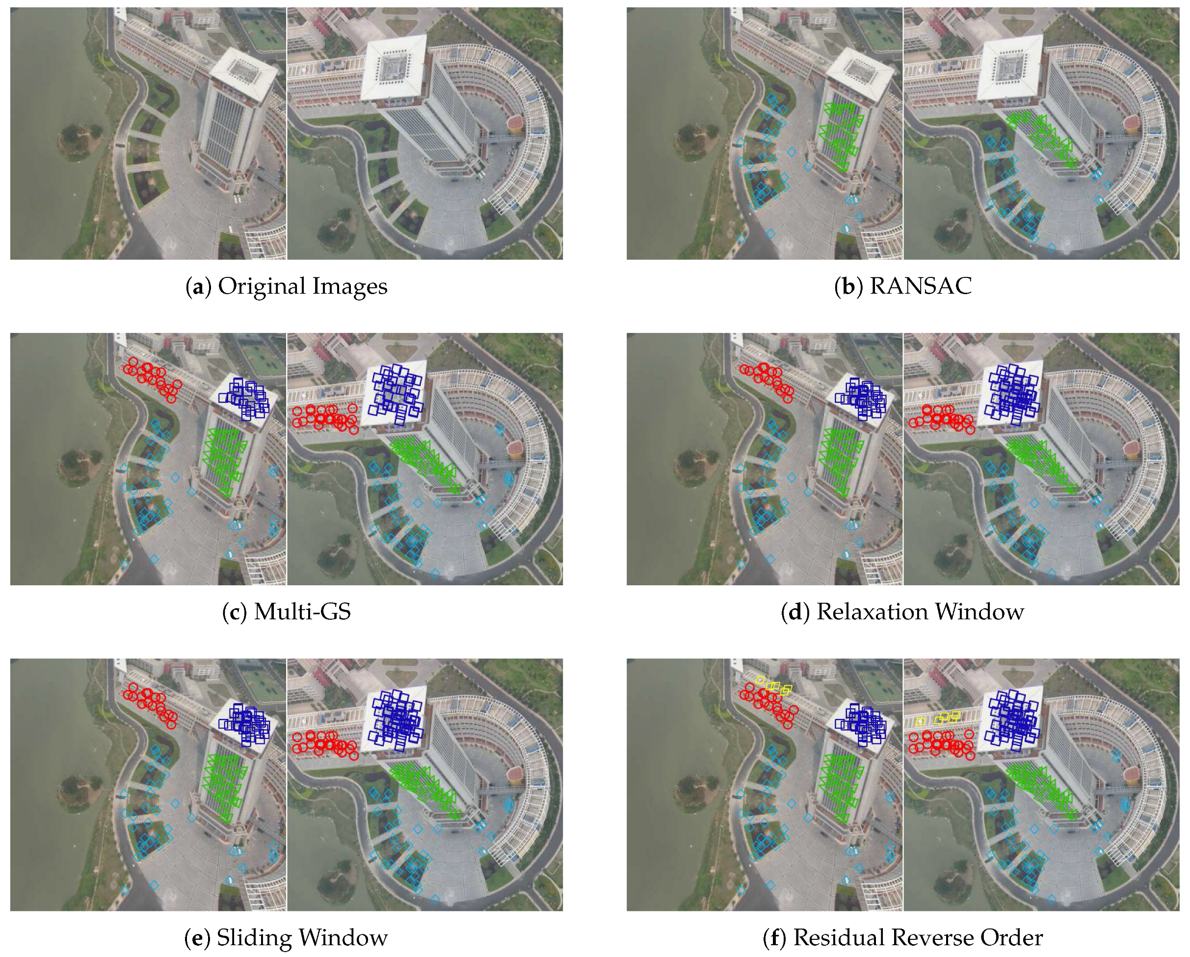
Figure 7.
The six-homographic matrices extracted from Library, where green triangles, blue squares, red circles, indigo diamonds, yellow parallelograms, and red triangles respectively represent inliers (correct matched features) that located on different planes in the scene.
Figure 7.
The six-homographic matrices extracted from Library, where green triangles, blue squares, red circles, indigo diamonds, yellow parallelograms, and red triangles respectively represent inliers (correct matched features) that located on different planes in the scene.

Figure 8.
The average sampling structures, the average number of valid structures, and the run time of hitting all structures.
Figure 8.
The average sampling structures, the average number of valid structures, and the run time of hitting all structures.

Figure 9.
Low-altitude UAV ariel high resolution image dataset.


Table 1.
The accuracy of fundamental matrix with seven methods.
| Image Category | Image | RANSAC | Multi-GS | RO | SW | RRO | RRO+RO | RRO+SW |
|---|---|---|---|---|---|---|---|---|
| Scale Change | Park | 0.7 | 0.5 | 0.5 | 0.5 | 0.6 | 0.6 | 0.7 |
| Roundabout | 0.8 | 0.7 | 1 | 0.9 | 0.5 | 0.8 | 0.9 | |
| Slight Viewpoint Change | Lecture Hall | 2.6 | 1.9 | 1.6 | 1.7 | 1.5 | 1.6 | 1.5 |
| Apartments 1 | 2.3 | 1.8 | 1.8 | 1.6 | 1.3 | 1.5 | 1.4 | |
| Bridge | 2.5 | 1.5 | 1.5 | 1.3 | 1.1 | 1.3 | 1.4 | |
| Severe Viewpoint Change | Hotel | 1.5 | 1.2 | 1.1 | 1.2 | 0.9 | 1.1 | 1.2 |
| Campus 1 | 3.2 | 2.1 | 1.9 | 2.5 | 1.7 | 2.0 | 1.7 | |
| Campus 2 | 2.1 | 1.3 | 1.3 | 1.1 | 1.1 | 1.1 | 1.1 | |
| Campus 4 | 2.7 | 2.0 | 1.9 | 1.8 | 1.4 | 1.3 | 1.6 |
© 2018 by the authors. Licensee MDPI, Basel, Switzerland. This article is an open access article distributed under the terms and conditions of the Creative Commons Attribution (CC BY) license (http://creativecommons.org/licenses/by/4.0/).
Share and Cite
MDPI and ACS Style
Cai, G.; Su, S.; Leng, C.; Wu, Y.; Lu, F. A Robust Transform Estimator Based on Residual Analysis and Its Application on UAV Aerial Images. Remote Sens. 2018, 10, 291. https://doi.org/10.3390/rs10020291
AMA Style
Cai G, Su S, Leng C, Wu Y, Lu F. A Robust Transform Estimator Based on Residual Analysis and Its Application on UAV Aerial Images. Remote Sensing. 2018; 10(2):291. https://doi.org/10.3390/rs10020291
Chicago/Turabian StyleCai, Guorong, Songzhi Su, Chengcai Leng, Yundong Wu, and Feng Lu. 2018. "A Robust Transform Estimator Based on Residual Analysis and Its Application on UAV Aerial Images" Remote Sensing 10, no. 2: 291. https://doi.org/10.3390/rs10020291
Note that from the first issue of 2016, this journal uses article numbers instead of page numbers. See further details here.