Evaluation of Coastal Sea Level Offshore Hong Kong from Jason-2 Altimetry

1
The CAS Key Laboratory of Microwave Remote Sensing, National Space Science Center, Chinese Academy of Sciences, Beijing 100190, China
2
Laboratoire d’Etudes en Géophysique et Océanographie Spatiales (LEGOS), Observatoire Midi-Pyrénées, 31400 Toulouse, France
3
State Key Laboratory of Remote Sensing Science, Institute of Remote Sensing and Digital Earth, Chinese Academy of Sciences, Beijing 100094, China
4
International Space Science Institute, 3102 Bern, Switzerland
*
Author to whom correspondence should be addressed.
Remote Sens. 2018, 10(2), 282; https://doi.org/10.3390/rs10020282
Submission received: 23 November 2017
/
Revised: 2 February 2018
/
Accepted: 6 February 2018
/
Published: 12 February 2018
(This article belongs to the Special Issue Satellite Altimetry for Earth Sciences)
Abstract
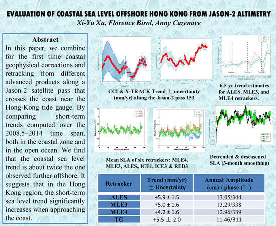
:As altimeter satellites approach coastal areas, the number of valid sea surface height measurements decrease dramatically because of land contamination. In recent years, different methodologies have been developed to recover data within 10–20 km from the coast. These include computation of geophysical corrections adapted to the coastal zone and retracking of raw radar echoes. In this paper, we combine for the first time coastal geophysical corrections and retracking along a Jason-2 satellite pass that crosses the coast near the Hong-Kong tide gauge. Six years and a half of data are analyzed, from July 2008 to December 2014 (orbital cycles 1–238). Different retrackers are considered, including the ALES retracker and the different retrackers of the PISTACH products. For each retracker, we evaluate the quality of the recovered sea surface height by comparing with data from the Hong Kong tide gauge (located 10 km away). We analyze the impact of the different geophysical corrections available on the result. We also compute sea surface height bias and noise over both open ocean (>10 km away from coast) and coastal zone (within 10 km or 5 km coast-ward). The study shows that, in the Hong Kong area, after outlier removal, the ALES retracker performs better in the coastal zone than the other retrackers, both in terms of noise level and trend uncertainty. It also shows that the choice of the ocean tide solution has a great impact on the results, while the wet troposphere correction has little influence. By comparing short-term trends computed over the 2008.5–2014 time span, both in the coastal zone and in the open ocean (using the Climate Change Initiative sea level data as a reference), we find that the coastal sea level trend is about twice the one observed further offshore. It suggests that in the Hong Kong region, the short-term sea level trend significantly increases when approaching the coast.
1. Introduction
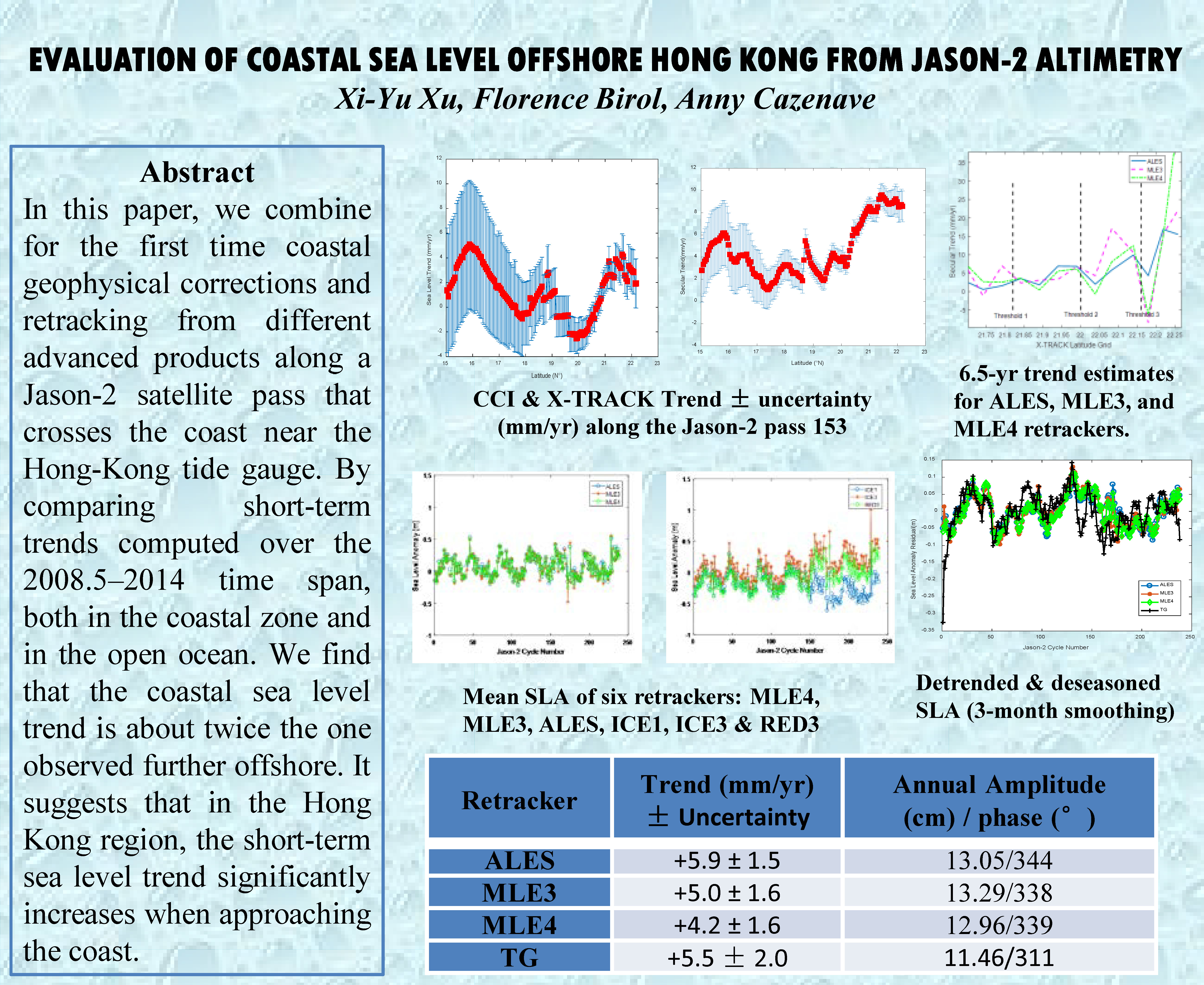
Sea level rise is one of the most threatening consequences of present-day global warming. About 10% of the world population currently lives in the world’s coastal zones and this number will increase in the future. Therefore, it is crucial to monitor and understand sea level variations along coastlines [1]. Although the tide gauge network has expanded in recent years, some highly populated areas like western Africa remain devoid of any station. For 25 years, satellite altimetry routinely monitored sea level changes over the global open ocean, but was largely unexploited in the coastal areas. Indeed, satellite altimetry was originally designed to precisely measure sea level in the open ocean, where the shape of the pulse-limited radar altimeter echo (i.e., after reflection on the sea surface; called waveform), is well described by the classical mathematical Brown model [2], based on the assumption of a homogeneous rough sea surface within the radar footprint. In that case, the sea level parameters (range between satellite and sea surface, significant wave height and backscatter coefficient) are extracted from the model via a Maximum Likelihood Estimation (MLE) approach. In a coastal band of a few kilometers wide (corresponding to the footprint size of the altimeter antenna), radar echoes integrate reflections from nearby land, leading to complex waveforms that significantly depart from the standard Brown model (e.g., [3,4,5] and references therein). Besides, in some shallow shelf areas, the sea surface might be so calm that the waveform can display several peaks due to specular reflection. Figure 1 shows two examples of waveforms, one over the open ocean (a) and the other in a coastal zone (b).
Another difficulty arises from the geophysical corrections applied to the altimeter measurements that usually suffer large uncertainties in the coastal zone. The most limiting corrections are wet tropospheric delay, ocean tides correction, dynamic atmospheric correction (DAC), and sea state bias. Near the coast, these corrections either have large spatio-temporal variability poorly reproduced by numerical models (e.g., tides and DAC corrections), or are less precisely estimated by onboard sensors than over the open ocean (e.g., the radiometer-based wet tropospheric correction that suffers severe land contamination). As a consequence, most altimeter data in a band of 10–30 km from land are declared invalid and discarded from the standard products. For about a decade, significant efforts have been realized by the altimetry community and space agencies to overcome this difficulty and retrieve as much as possible historical altimeter measurements near the coast. Corresponding coastal altimetry products are based on improved coastal geophysical corrections [6,7] and/or dedicated analysis approaches to extract the sea level parameters (range, significant wave height and backscatter coefficient) from non-standard waveforms (a process called ‘retracking’) [3,4,5].
In this study, we investigate the relative performances of the experimental coastal altimetry products available for the Jason-2 mission. Jason-2 is chosen here because it was consistently operating for nearly one decade and, above all, because it has been reprocessed by most of the coastal altimetry groups. Satellite pass 153 is considered. We used the following coastal altimetry products: (1) X-TRACK [6] developed by LEGOS (Laboratoire d’Etudes en Géophysique et Océanographie Spatiales, France); (2) PISTACH (Prototype Innovant de Système de Traitement pour l’Altimétrie Côtière et l’Hydrologie, [8]) developed by CLS (Collecte Localisation Satellites, France); and (3) ALES (Adaptive Leading Edge Sub-waveform, [3]) developed by NOC (National Oceanography Centre, UK). The products propose either improved geophysical corrections or waveform retracking algorithms, thus have different contents. X-TRACK products provide sea level time series on a nominal mean track and are available for all altimeter missions except HY-2A and Sentinel-3A. ALES products provide products for Jason-2 and Envisat missions. The successor of the PISTACH product, PEACHI (Prototype for Expertise on Altimetry for Coastal, Hydrology, and Ice), is dedicated to the SARAL/AltiKa mission and provides sea level data along original, cycle-by-cycle tracks [9]. Because of these important differences between products, very few attempts to inter-compare coastal sea level data have been carried out so far, despite the importance of this type of exercise for defining the best processing strategy to derive coastal altimetry data.
In this paper we focus on the South China Sea (Hong-Kong area), not only because of a variety of climate processes impacting sea level (ENSO–El Niño Southern Oscillation-, eddies, storm surges, monsoon, etc.), but also for its importance in the economy and security of Southeastern Asia and the Western Pacific regions. An important consideration when selecting the study area was also the availability of external tide gauge-based sea level data for validation. A dozen tide gauges exist along the China coast, but all stations located along the Chinese mainland ceased to provide data after 1997. Fortunately, a tide gauge remained in operation during the Jason-2 mission at Quarry Bay, Hong-Kong. Corresponding hourly data are available from the University of Hawaii Sea Level Center (UHSLC) [10]. In this study, we considered the closest Jason-2 satellite track (which is ascending and numbered 153) of the HK tide gauge (10.05 km away).
2. Study Area
Hong-Kong (HK) is located just south of the Tropic of Cancer. The climate is predominantly subtropical and displays clear seasonal variations. The southwesterly/northeasterly monsoon give rise to warm wet summers and cool dry winters. HK is also frequently impacted by typhoons. On the western side of the HK island flows the Zhujiang River (Pearl River), which brings abundant freshwater (~3.5 × 10¹¹ m3 per year [11]), resulting in a high salinity gradient. All these factors increase the complexity of the HK environment and have an impact on the regional sea level variations at different spatio-temporal scales.
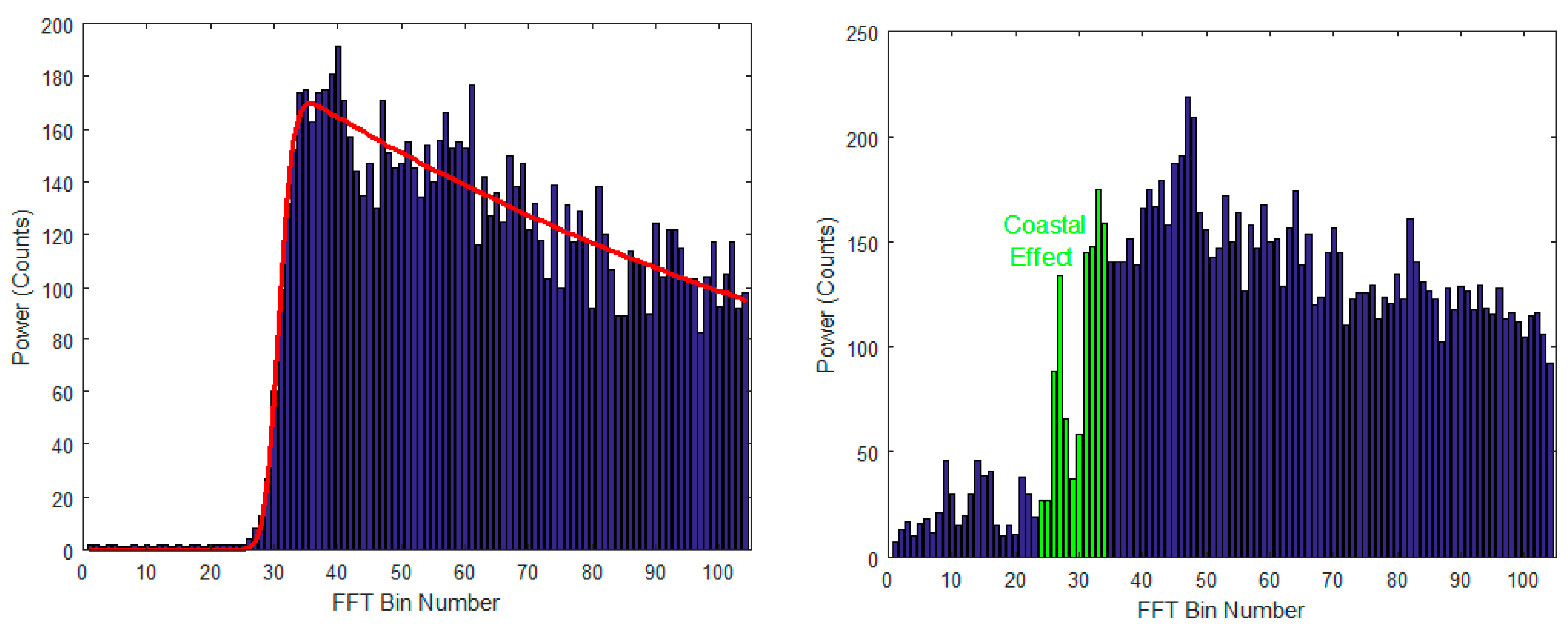
The HK coast has also an extremely complex geomorphology. As shown on Figure 2, tiny islands lie within the radar footprint of the Jason-2 track chosen for this study. As a consequence, the corresponding altimeter and radiometer measurements are expected to be severely impacted by land effects. This makes this area particularly relevant for analyzing the performances of coastal altimetry data.
The definition of the “coastal zone” in altimetry is somewhat arbitrary. In some studies the criteria of 50 km from land is used (for example, ALES data are provided only in the 50-km coastal band), while some others focus on the first 10 km or even 5 km off the coastline. In this paper we have chosen to base the definition of the area on the “rad_surf_type” parameter provided in the Geophysical Data Record products (GDRs). This surface classification flag is derived from the radiometer measurements and indicates the type of observed surface. For the Jason-2 pass #153, the coastal area based on this flag corresponds to the area where the satellite flies less than 70 km from the closest land (including small islands).
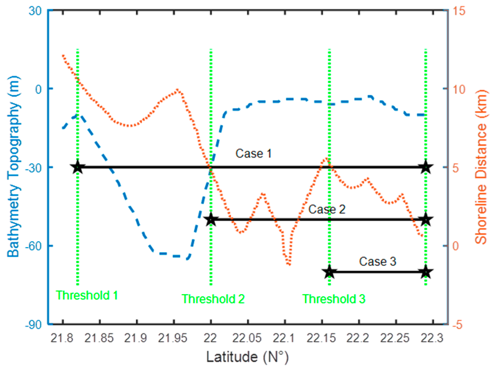
The HK coastal topography is extremely irregular. Figure 3 shows a bathymetric profile along the Jason-2 pass, from southwest to northeast (blue dashed line; from 21.8°N to 22.3°N latitude). Despite a narrow band between 21.8°N and 22°N, where the depth is steeply falling down to ~−60 m, the study area corresponds to very shallow waters. We can thus expect complex local tides and currents influencing sea level variations. Figure 3 also shows the corresponding along track distance to land (mainland or island). The “distance to land” profile is rather complicated. Coastward, it first decreases to ~8 km, slightly increases to ~10 km, and then fluctuates between 10 and 0 km. It even reaches ~0 km when the satellite flies over a small island called Wailingding Island (see Figure 2). Considering both distance to coast and water depth, we define three cases for our comparison exercise, corresponding to three different overlapping segments along the Jason-2 pass. Segments 1, 2, and 3, correspond to cases 1, 2, and 3. In Figure 2, these can be identified by the orange, green, and dashed blue colors, respectively. They cover distances of 50 km, 30 km, and 10 km, and reflect increasing coastal conditions (thus increasing difficulty to retrieve a coherent physical signal from altimetry data). For each case, each satellite cycle, and each product analyzed, we spatially averaged all available 20-Hz (~0.3 km resolution) along-track sea level data along the corresponding pass segment (up to the last valid measurement at HK coast). We finally obtained three mean sea level values for each product and each date. The corresponding altimetry-based sea level time series were then compared with the tide gauge data for validation.
3. Data Sets
The Jason-2 mission started operating in July 2008, while the high-quality tide gauge data were accessible until 2014 only. Besides, the ALES data were available for cycle 1 to 252 (July 2008 to May 2015). These constraints define the study time period: from July 2008 to December 2014, corresponding to cycles 1-238 of Jason-2 satellite, i.e., a time span of 6.5 years.
3.1. Coastal Altimetry Data Sets
3.1.1. General Description
The experimental coastal Jason-2 products analyzed in this study are X-TRACK (CTOH/LEGOS, [6]), ALES (PODAAC, [3]) and PISTACH (CNES, [8]). These data sets are available from the following websites: ftp.legos.obs-mip.fr; ftp://podaac.jpl.nasa.gov/allData/coastal_alt/L2/ALES and ftp://ftpsedr.cls.fr/pub/oceano/pistach.
We have to keep in mind the differences between the products considered in this study. X-TRACK is a level 3 (L3) product: using the GDR data and state-of-the-art altimetry corrections, along-track sea level time series projected onto reference tracks (points at same locations for every cycle) are computed at 1-Hz (~6 km along-track resolution). Both a raw and a spatially filtered version (40 km cutoff frequency) of the product are distributed. It is simple to use, and is based on improved geophysical corrections near the coast (see [6] for details) but its current version only includes the standard MLE4 retracker adapted to open ocean conditions. ALES and PISTACH are level 2 (L2, i.e., cycle-by-cycle) products: the measurements are provided at 20-Hz (~0.3 km along-track resolution) and are not projected onto reference tracks, which means that their location varies from one cycle to another (this processing step needs to be done by the user). The ALES and PISTACH products do not include improved geophysical corrections, but provide altimeter range estimates obtained using different retracking algorithms (Section 3.1.2). PISTACH also includes a classification of the altimeter waveforms which can be used to study the type of waveform analyzed. It also indicates if the waveform shape is consistent to the retracker used.
3.1.2. Waveform Retrackers
Waveform retrackers can be classified into two categories: physically-based retrackers and empirical retrackers [12]. The model-free retracker is purely based on the statistics of the waveforms and does not require any echo model. Among the multiple model-free retrackers available, the improved threshold retracker [13] is usually considered as the best one. It combines the advantages of the OCOG (Offset Center of Gravity, [14]) and simple threshold [15] algorithms.
Over the last decade, a new approach called “sub-waveform” has been developed. It consists of fitting only the portion of the waveform that contains the leading edge but excludes the trailing edge where most artifacts appear (e.g., [3,8,16,17,18]).
The retrackers that are available in the different L2 products are summarized in Table 1. The standard GDRs include two solutions: MLE3 and MLE4. The rationale of these two retrackers is similar: fitting the waveform to a Brown model based on the MLE (essentially non-linear least squares) techniques. The main difference between them is the number of parameters included in the model. MLE3 estimates three parameters: epoch (i.e., altimetric range), Significant Wave Height (SWH) and amplitude (i.e., backscatter coefficient-sigma-0), while MLE4 also retrieves the square of off-nadir angle.
The PISTACH products provide four retrackers: OCE3, RED3, ICE1, and ICE3 [8]. OCE3 is essentially the same as the MLE3 parameters in the GDRs. ICE 1 is a modified threshold retracker. RED3 and ICE3 are the counterparts of OCE3 and ICE1 respectively, where the retracker is executed in a sub-waveform version instead of on the entire waveform.
ALES is based on an advanced retracker called sub-waveform retracker [3]. It is an improved version of RED3, and the difference between them is the estimation of the sub-waveform. In RED3, the sub-waveform has always 31 bins (t0 + [−10:20], where t0 is the 32nd bin of the entire waveform), while in ALES, the sub-waveform length can vary from 39 bins (for SWH = 1 m) to 104 bins (i.e., the entire waveform, for SWH ≥17 m). In practice, the content of the ALES product is the same as the standard SGDR product (Sensor GDR) plus seven additional parameters specific to to the ALES retracker.
3.1.3. Geophysical Corrections
In PISTACH and X-TRACK, state-of-the-art geophysical corrections other than those of the official GDR are provided. For X-TRACK, only the ocean tide solution and the DAC are provided individually, while in PISTACH, two to three values are given for each correction. Different sets of correction terms obviously lead to different coastal sea level estimates.
3.2. Tide Gauge Data
The Quarry Bay tide gauge is a float-type instrument. It provides sea level data with an accuracy of 1 cm for a single measurement and is regularly calibrated every other year [19]. The tide gauge is located at 114.22°E, 22.28°N, near the northern coast of the HK Island, separated from the Kowloon Peninsula by the Victoria Harbor (see Figure 2). Note that ~95% of the Victoria Harbor shoreline is shaped by human activity [11]. Thus sea level on this area is likely influenced by anthropogenic local-scale factors, in addition to more regional and global ocean variations. Hourly tide gauge data were downloaded from the Sea Level Center of the University of Hawaii (https://uhslc.soest.hawaii.edu).
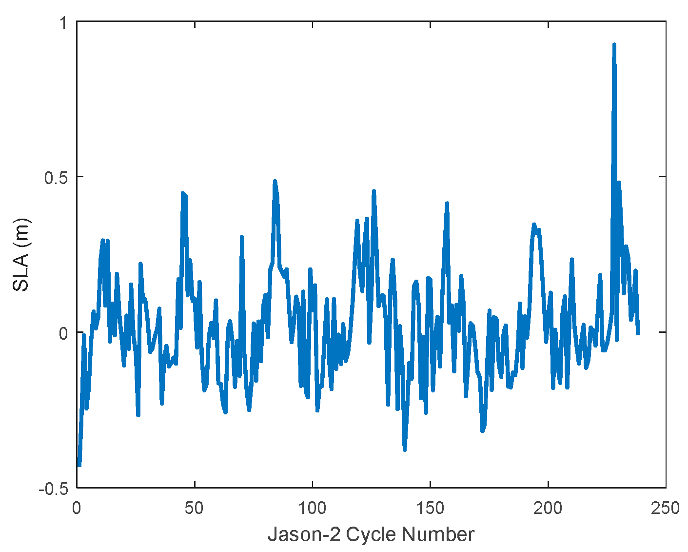
A harmonic analysis was first applied to the tide gauge data in order to compute and remove the tidal signals from the sea level time series. A time-averagedsea level value was also removed from the time series in order to be consistent with the altimetry sea level data. Finally, the hourly tide gauge data were interpolated to the time of the Jason-2 observations. Note that the dynamic atmospheric correction was not removed from the tide gauge data. This will be discussed in Section 5.5. The tide gauge-based sea level time series interpolated to the closest Jason-2 observations is shown in Figure 4. We observe a large seasonal cycle, due to the monsoon, modulated by important high-frequency variations which can reach several tens of cm. In particular, a peak is observed at cycle 228. It is caused by a storm surge associated with the violent Typhoon Kalmaegi that sideswiped the HK coast before dawn on 16 September 2014. The Jason-2 altimeter flew over the HK area at 3.45 am (local time) on 16 September 2014, and the peak in the tide gauge sea level series is coincident with the typhoon event. Therefore, this peak was eliminated in our analysis as an outlier.
3.3. ESA Climate Change Initiative (CCI) Sea Level Data
Global altimetry sea level data sets are regularly produced by different groups worldwide. Five of them are solely based on the TOPEX-Poseidon/Jason-1/2/3 satellites (reference missions): AVISO (Archivage, Validation et Interprétation des données des Satellites Océanographiques) in France, NOAA (National Oceanic and Atmospheric Administration), GSFC (Goddard Space Flight Center) and CU (University of Colorado) in the United States, and CSIRO (Commonwealth Scientific and Industrial Research Organization) in Australia. The Climate Change Initiative (CCI) sea level (sl_CCI) project of the European Space Agency (ESA) has been developed in the recent years to realize the full potential of multi-mission altimetry as a significant contribution to climate research [20,21,22]). In the context of the CCI, altimetry missions have been reprocessed using improved geophysical corrections and improved links between missions, providing reduced errors of sea level products. In this study, we use the sl_CCI (v 2.0) data from July 2008 to December 2014 to estimate sea level trends in the open ocean away from the HK coast. The sl_CCI v 2.0 data set is a gridded product at 0.25° × 0.25° resolution. The Sl_CCI project was not dedicated to estimate sea level near the coast. However, it can be used as a good independent reference to link open ocean sea level variations to coastal altimetry sea level, thus providing a regional context to interpret the coastal results obtained in this study.
4. Methodology
4.1. Altimetry Data Processing
As indicated above, current coastal altimetry products differ in terms of content. Thus a first step consists of processing the different data sets to obtain homogeneous variables for further comparison. Because there is no waveform data in PISTACH, we used the waveforms provided in ALES, and merged PISTACH and ALES using the measurement time common to all products. In Section 5.4, we also projected all along-track, cycle-by-cycle L2 data onto the X-TRACK 1-Hz reference grids to benefit from the XTRACK improved geophysical corrections.
4.1.1. Sea Level Anomaly (SLA) Estimation
From the altimeter range, once all the propagation and geophysical corrections mentioned below are removed, we can deduce the sea surface height (SSH, i.e., sea level referred to a reference ellipsoid). If we further remove a mean sea surface in order to overcome the problem of geoid estimation, we obtain sea level anomaly (SLA) data. In this study we use SLA data, computed as follows:
SLA = H − R − ΔRiono − ΔRdry − ΔRwet − ΔRssb − ΔRtide − ΔRDAC − MSS
In Equation (1), H is the orbital height, R is the Ku-band altimeter range, ΔRiono is the ionospheric correction, ΔRdry and ΔRwet are the dry and wet tropospheric corrections, respectively, ΔRssb is the sea state bias, ΔRtide is the tide correction (composed of the ocean tide, pole tide and solid Earth tide), ΔRDAC is the dynamic atmospheric correction, and MSS is mean sea surface (in practice we used the MSS_CNES_CLS-2011 model).
In some cases, R is not directly available (for instance, there is no specialized range parameter in the ALES product), so it can be computed as follows:
where T is the onboard tracking range in the Ku band, E is the retracked offset (with time dimension), the factor “c/2 (c is light velocity)” is the scaling factor from traveling time to range, D is the Doppler correction in Ku band, M is the instrument bias due to PTR and LPF features ([23,24] and 0.180 is a bias (in meters) due to wrong altimeter antenna reference point [25].
R = T + E × (c/2) + D + M + 0.180
In this study, we computed SLA time series using the altimeter ranges issued from six retrackers: ALES, MLE3, MLE4, RED3, ICE1, and ICE3. For the MLE3, MLE4, and ALES retrackers, we first used Equation (2) to compute R, and then applied Equation (1) to compute the SLA (because R is often flagged in the GDR and ALES products). To validate our calculation method, we compared the MLE4 SLA obtained with the equivalent official “ssha” parameter provided in the GDRs, and found good consistency. For RED3, ICE1, and ICE3, we applied Equation (1) to directly compute the SLA, because there were no valid E values in the PISTACH product.
4.1.2. Choice of the Geophysical Corrections
The geophysical corrections near the coast also need specific considerations. The first error source comes from the wet tropospheric correction because the onboard radiometer suffers from land contamination in the coastal area. A simple but effective approach is to extrapolate a model-based correction (using for example atmospheric reanalyses from the European Center for Medium-Range Weather Forecasts, ECMWF) but the corresponding spatial resolution is relatively low for coastal applications. Other approaches include an improved radiometer-based correction accounting for the land contamination effect [26], or the computation of GNSS-derived Path Delay (GPD, [27]). Since the GPD has not been included in the current versions of the three coastal products analyzed here, we used the decontaminated radiometer solution provided in PISTACH.
Concerning the ionospheric correction, the imperfect coastal altimeter range measurements lead to significant errors, generating outliers in the correction values. We use the MAD (median absolute deviation) technique described in detail in Section 4.1.3 to detect and remove the outliers. The along-track profile of ionospheric corrections is further spatially low-pass filtered using a LOESS (LOcally Estimated Scatterplot Smoothing) method with a cutoff frequency at 100 km.
The coastal ocean tide corrections, provided by global models, are also far from accurate. There are five different ocean tide solutions available in the products, computed by two scientific teams: (1) the Goddard Ocean Tide (GOT) models developed by Ray et al. [28], and the Finite Element Solution (FES) models developed by Lyard et al. [29]. Two ocean tide solutions are provided in the official GDRs: GOT4.8 and FES2004. PISTACH contains two older versions of GOT: GOT00.2 and GOT4.7 as well as an upgraded version of FES: FES 2012. In Equation (1) we adopt the GOT4.8 ocean tide solution.
Ray [30] compared different tide solutions against 196 shelf-water tide gauges and 56 coastal tide gauges. Their accuracy was characterized by the RSS (root sum square) error of the eight main tidal components (Q1, O1, P1, K1, N2, M2, S2, K2). For the shelf-water gauges, the accuracy of GOT4.8 was 7.04 cm along European coasts and 6.11 cm elsewhere, while the accuracy of FES2012 was 4.82 cm and 4.96 cm respectively for the European coasts and elsewhere. For the coastal tide gauges, the accuracy of GOT4.8 and FES2012 were 8.45 cm and 7.50 cm respectively. In comparison, the accuracy of GOT4.7 and FES2004 in shelf-water were 7.77 cm and 10.15 cm respectively. These results illustrate the significant improvement in coastal ocean tide solution during the last 10 years. In Section 5.5, we also compare three tide solutions, GOT4.8, FES 2004, and FES 2012, to assess their relative performances.
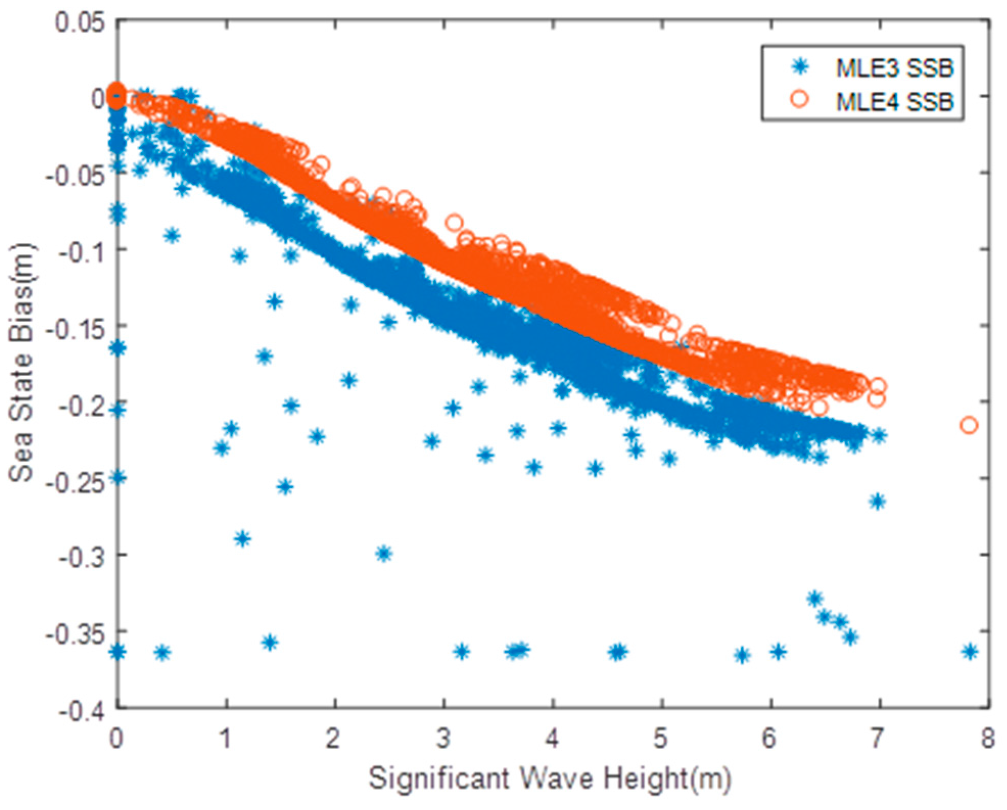
Another important altimetry correction is the sea state bias (SSB). The SSB depends on the retracking algorithm, because it contains the tracker bias. A careful analysis showed that for Jason-2 GDRs, the SLA obtained from MLE3 and MLE4 retrackers has large bias. From a statistical analysis based on cycles 1 to 238 for a couple of altimeter passes over the open ocean, we obtained: SLAMLE3 − SLAMLE4 = +2.3 cm. Near the coast, this bias appeared to be even larger and even more critical as it was not constant. Figure 5 shows both MLE3 and MLE4 SSB corrections as a function of SWH for an arbitrary pass (cycle 16, pass #153). MLE3 SSB has a clear bias (~+3 cm) relative to MLE4 SSB. Moreover, MLE3 SSB seems to have many outliers, in particular near the coast. We concluded that the bias observed between MLE3 and MLE4 sea level estimates corresponds to a bias in the SSB corrections.
Deeper investigation showed that the MLE3 SSB outliers are often related to large off-nadir angle values (not shown), probably erroneous given the good attitude control of Jason-2. For that reason, we adopted the MLE4 SSB in the computation of all SLAs, resulting in a relative bias <1 cm for all retrackers.
In Equation (1), some parameters are available at 20-Hz (e.g., E), and others at 1-Hz (e.g., D). We interpolated all 1-Hz parameters at 20-Hz and finally computed 20-Hz SLA. The 20-Hz SLA is more useful for the retracker performance analysis, and can also be used for subtle feature detection.
4.1.3. Data Editing Strategy
Near the coast, the number of outliers in data sets is obviously much larger than over the open ocean. Thus the data must be edited before being used. The outliers are detected and removed using the MAD filter. It is based on the median value of the data analyzed, which is more robust than the mean value in the presence of outliers. For a Gaussian random signal, MAD is defined as:
where σ is the standard deviation of the data. For the Chauvenet’s criterion (0.5% outliers for a Gaussian series, [31]), it will be appropriate to set a threshold of 2.81 × σ, equivalent to 3.52 × MAD.
Therefore, values satisfying:
are defined as outliers. This is very similar to the criterion (3.5 × MAD) adopted by Birol et al. [6] in the ionospheric correction editing process of the X-TRACK product.
Objectively, all outliers cannot be thoroughly detected by the above criterion. In the presence of distorted waveforms, retrackers such as ALES can occasionally produce unrealistic SLA values, up to tens of meters and hence increase the MAD. Some outliers may remain after editing in this case. So we have defined a threshold value before applying the MAD editing. All the SLA values beyond ±2 m are deleted. Some high amplitude real oceanographic features (such as storm surge) may also be deleted. But for the purpose of the present study, the storm surge events can be removed from the analysis. Finally, almost all outliers are detected after this threshold is applied.
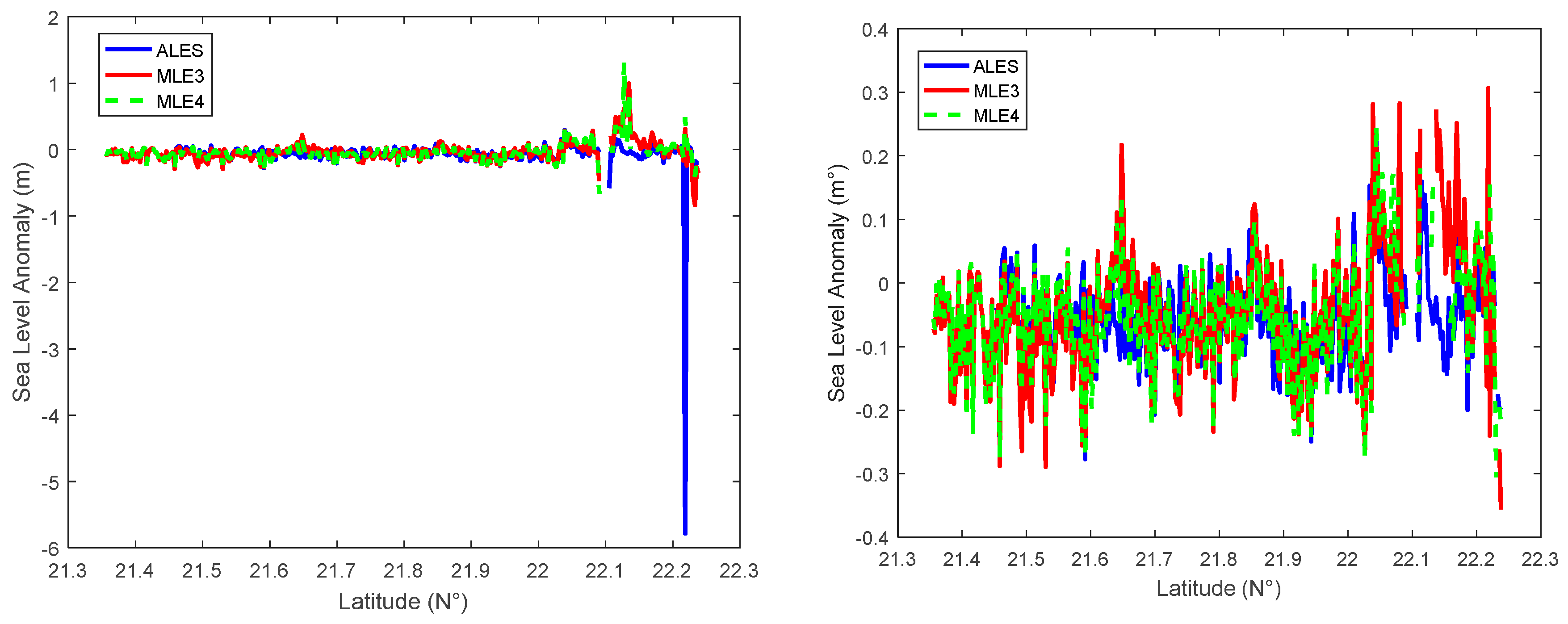
A typical along track profile of 20-Hz SLA before and after editing is shown in Figure 6 for a given cycle (cycle #5 is arbitrarily chosen here). ALES is not as robust as the MLE algorithms for the last few coastal measurements: it has many outliers in almost all cycles (in fact, the mean number of outliers beyond ± 10 m in ALES is ~9 per cycle, much larger than for MLE3 or MLE4). However, after editing, ALES performs better than MLE3 and MLE4, since it displays the lowest noise level.
4.2. Sea Level Data Analysis
After computing the SLA for each cycle and each retracking, the time series can be analyzed to retrieve useful oceanography information. Because of the monsoon, the annual and semi-annual signals are both significant near the HK coast. Therefore, at a first order, SLA variations can be modeled as follows:
where Tyear = 365.2425 days, ε(t) is the residual SLA, a1 to a6 are the regression coefficients to be estimated: a6 is a bias, a5 is the sea level trend, the annual/semi-annual amplitude and phase can be deduced from a1 to a4:
Coefficient uncertainty is defined as the square root of the diagonal elements in the covariance matrix of the coefficient vector.
In practice, we estimated the seasonal terms and trend separately: the seasonal coefficients were removed first from the detrended time series; then the short-term trend was estimated from the residuals (i.e., initial time series corrected for the seasonal terms) after reintroducing the initial trend. In the latter step, a nine-point moving window (corresponding to an about 3-month cutoff frequency) was applied to the residuals to reduce the intrinsic 59-day erroneous signal presented in Jason altimetry missions [32,33].
Note that the computed trends based on only 6.5 years of data essentially represent the inter-annual variability. These short-term trends are expected to be significantly different for long-term trends estimated over the whole altimetry era. In the following the term ‘trend’ means ‘short-term trend’. In this work, it is used as a diagnostic to analyze the quality of near-coastal altimetry data and not the long term sea level trend related to climate change.
5. Results
5.1. A First Analysis Based on Jason-2 Waveforms Observed along the Track
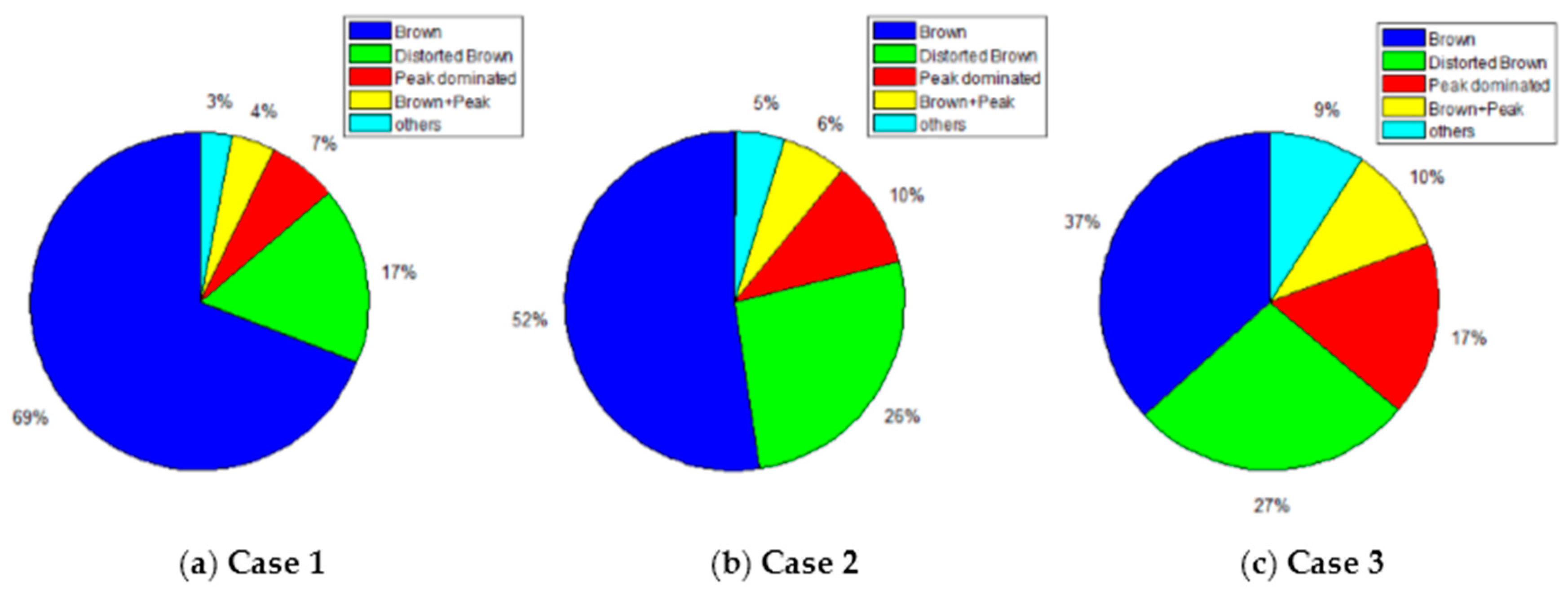
The HK coast considered in this study has a very complex topography, so the waveforms are diverse. In order to go further in our analysis we used the waveform classification provided in the PISTACH product. It classifies the altimeter waveforms into 16 classes, including a “doubt” class. Based on considerations on all waveform shapes, we grouped these classes into five categories (see Table 2). In Table 2, for each category, we provide a general description of the surface observed and propose a specific retracker.
We use these five categories to classify all Jason-2 waveforms used in our study. The resulting percentages of waveforms as a function of category and case (i.e., distance to the coast) are shown in Figure 7. In all three cases the most frequent category is “Brown”, and the second is “Distorted Brown”. Not surprisingly, the percentage of Brown-like waveforms decreases when approaching land. In case 2, more than 52% of the waveforms are Brown-like and in case 3 this number decreases to 37%. Concerning the distorted-Brown waveforms, logically, their percentage increases when the distance to the coast decreases. It varies from 17% in case 1 to 27% in case 3. These results suggest that within a shoreline distance of 5 km, a significant number of waveforms are Brown-like and that using a classical open-ocean retracker can still provide good quality sea level data in this very nearshore area. However, the use of ALES is expected to increase the number of retrieved accurate data, which is what we found in the previous section.
5.2. Sea Level Trend
5.2.1. A regional View
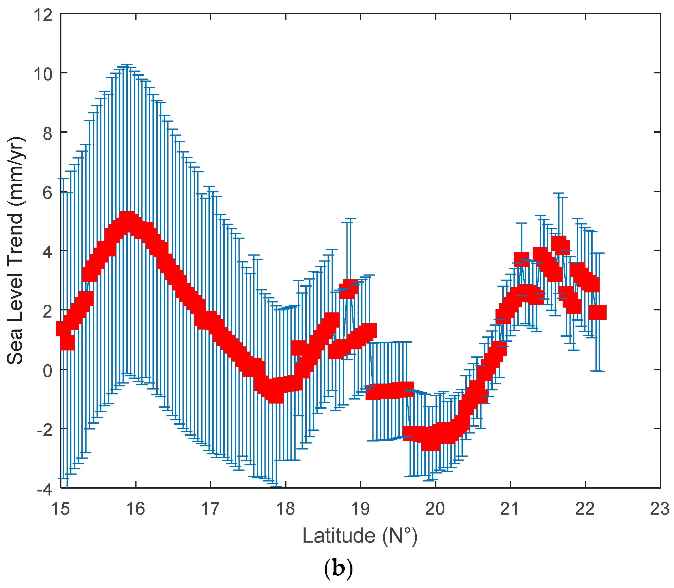
We first used the gridded CCI sea level data to obtain a regional picture of the sea level trends from July 2008 to December 2014 (Figure 8a). To compare the gridded CCI sea level with the coastal sea level estimated in this study (see below), we interpolated the CCI trend grid along the Jason-2 pass at 1-Hz resolution (~7 km). Corresponding CCI-based along-track sea level trends are shown in Figure 8b. The uncertainty associated with the trend estimation is also provided (blue bars). These error bars are rather large because the time span of analysis is short and the inter-annual variability is large. Trend estimates using the whole CCI altimetry record (i.e., 23-years, from January 1993 to December 2015) display much smaller errors, but a behavior similar to Figure 8b is also observed, i.e., larger errors around 16°N than near the coast.
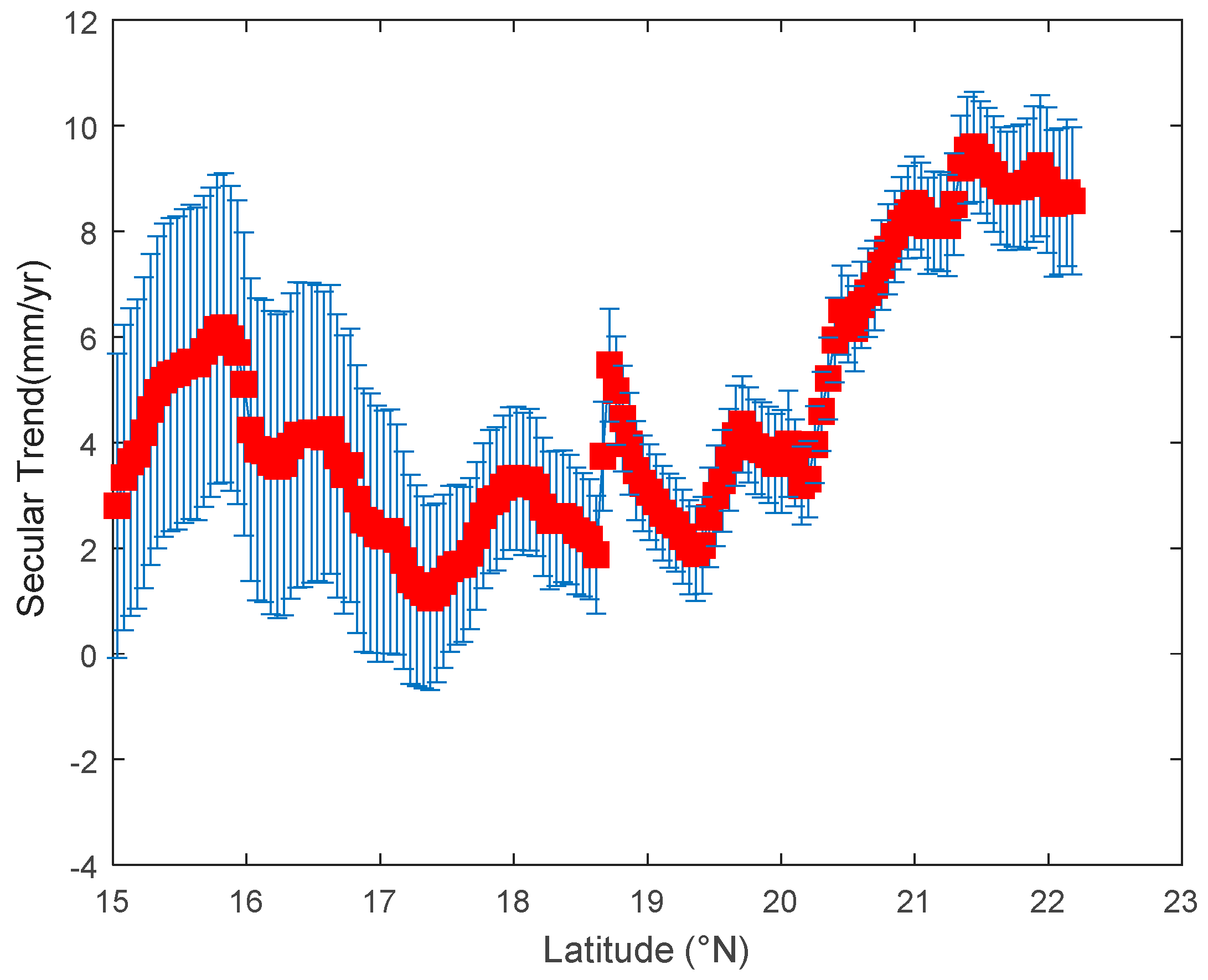
In parallel, in order to see the impact of the different altimetry products used here (thus of the different data processing) on the results, the linear 6.5-year trends were also estimated along the Jason-2 pass from both the raw and filtered versions of the X-TRACK SLA time series. Results obtained from the filtered X-TRACK SLA are shown in Figure 9 as a function of latitude.
From Figure 8 and Figure 9, we observe a significant spatial variability in the regional sea level trends. The CCI map (Figure 8a) displays values of −6 to −4 mm/yr over the open ocean which tend to increase to +2 to +4 mm/yr near the coast. Figure 8b illustrates how Jason 2 pass 153 captures part of this regional trend pattern, with values varying significantly from −2 mm/yr to +4 mm/yr along the track. In X-TRACK (Figure 9), around 20°N, the linear trend is also relatively small (~2–3 mm/yr), in agreement with the CCI data. A change is observed near 19°N, corresponding to the along-track influence of a narrow trench (the bathymetry rapidly decreases to ~−2500 m and then recovers to ~−100 m). As in the CCI data, the X-TRACK trends increase towards the coast but the values obtained in the vicinity of HK are much larger than for the CCI trends: +8 to +9 mm/yr against +2 mm/yr. The sea level trend at the last point of the filtered X-TRACK SLA is: +8.6 ± 2.2 mm/yr. However, gridded altimetry products, such as in the CCI data set, have too low resolution to capture near-shore sea level variations. This also explains why the trends of the gridded CCI data have larger uncertainty than the unsmoothed X-TRACK data.
5.2.2. The Tide Gauge Reference
Using Equation (5), we computed the tide gauge trend over the 6.5-yr time span considered in this study. We found a linear sea level trend value of +5.2 ± 2.0 mm/yr (after eliminating the outlier corresponding to the storm-surge event). However for further comparison with the altimetry-based sea level data, the tide gauge time series needs to be corrected for vertical land motion (VLM) [36]. This can be done using GPS precise positioning techniques. Yuan et al. (2008) [37] analyzed data from a GPS station named HKOH, which is close to the tide gauge. VLM at HKOH was estimated to +0.22 ± 0.46 mm/yr. Lau et al. (2010) [38] analyzed GPS data (2006–2009) from HKOH and obtained a VLM estimate of +0.3 mm/yr (uncertainty not provided). The time spans of these studies are different from ours, but because the VLM at HK appeared to be fairly stable over the last decade, we assume a VLM value of +0.3 mm/yr. After correcting for VLM, we find a trend of +5.5 ± 2.0 mm/yr at the tide gauge site.
5.2.3. Solutions Derived from the Different Retrackers
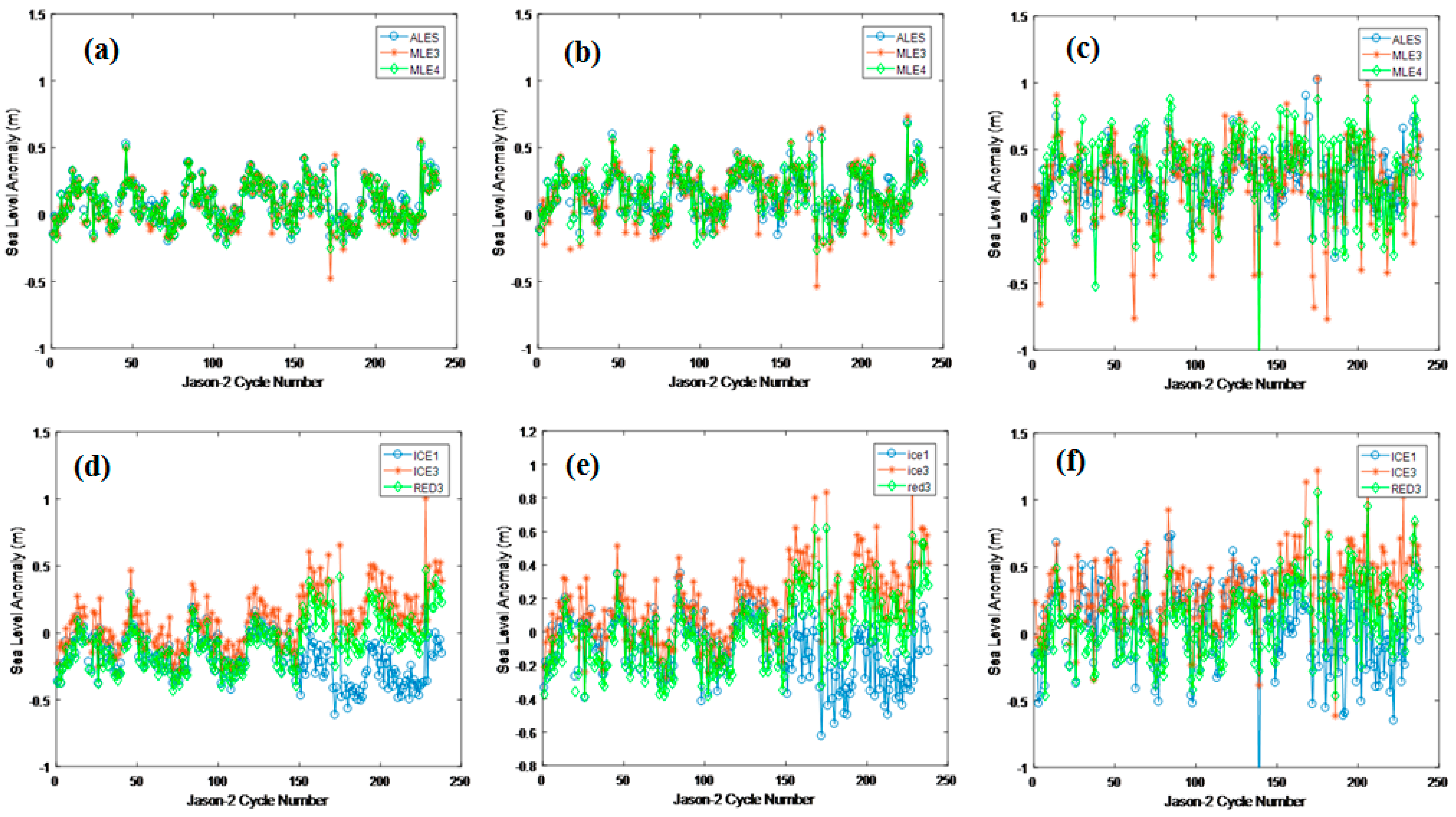
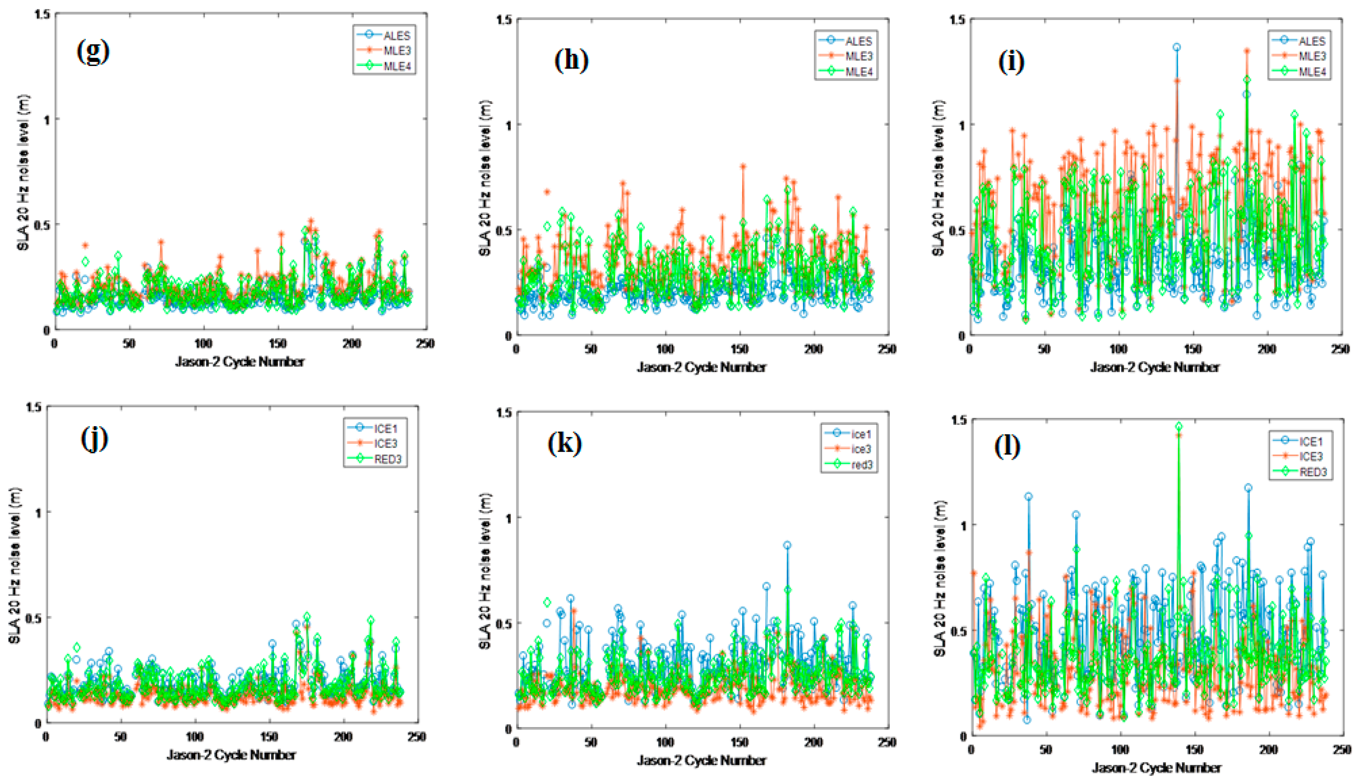
For each of the three cases defined in Section 2 and each retracker, we computed a spatially averaged 20-Hz SLA time series (see Section 4.1.1) as well as the associated 20-Hz noise level (estimated by the standard deviation of the 20-Hz SLA series). The results are shown in Figure 10. In all cases, ALES solution provides the lowest noise level after editing, and MLE4 is slightly less noisy than MLE3. Concerning the three experimental retrackers used in PISTACH, ICE3 has the lowest noise level, and RED3 is slightly less noisy than ICE1.
Note that a problem was detected in some of the PISTACH SLA solutions: around cycle #150, both ICE3 and RED3 have much larger SLA than ICE1, the relative bias being about 0.2 m. Comparison with the tide gauge sea level showed that ICE1 SLA roughly followed the tide gauge data, while ICE3 and RED3 data display large jumps. The latter severely influences the corresponding sea level trend estimates.
Sea level trends obtained from Equation (5) are summarized in Table 3 (except for OCE3 in PISTACH, which is the same as MLE3).
From Table 3 we note that, using the tide gauge as reference, case 1 provides the closest estimate to the tide gauge trend. Besides, we note a difference of less than 1 mm/yr for ALES and M LE3. This can easily be explained. As shown in Figure 2, case 2 includes a number of small islands while case 1 contains more land-free areas, thus more accurate SLA data. Finally, case 3 has very few valid altimetry measurements (usually less than five valid points), which is not enough to provide robust results.
MLE3 and ALES trends are both close to the tide gauge trend (within 0.5 mm/yr). The trends estimated from MLE4 are slightly lower than for ALES and MLE3 but the difference is within the error bar. The trends deduced from the PISTACH retrackers highly disagree with the tide gauge trend: both ICE3 and RED3 show unrealistic large values (>+5 cm/yr), while ICE1 shows a negative trend of −2 cm/yr. The ICE1 retracker may be inherently not accurate enough to derive trends, but concerning ICE3 and RED3 retrackers, since the processing procedure used in this work is homogeneous, the large errors may not come from the retracker algorithm itself, but more likely from errors in the basic products. For example, in a new PISTACH version, the 18 cm calibration bias used in Equation (2) may no longer be applied in the computation of R. Since the retracked offset E parameter is no more accessible in the current PISTACH version, this hypothesis could not be verified. Anyway, in the remaining part of the study we discard ICE1, ICE3, and RED3 solutions and concentrate on MLE3, MLE4, and ALES which, in the context of our study, appear as the best available retrackers to capture coherent coastal sea level signals from altimetry.
5.3. Coastal Seasonal Signal along the Jason-2 Pass
Using Equation (5) we also computed the amplitude and phase of the seasonal signal for all sea level time series. The resulting values are shown in Table 4 (for the annual signal) and Table 5 (for the semi-annual signal). All three cases give rather similar results that agree well with X-TRACK. The annual phases lie between 300°–360° and are significantly larger than the tide gauge-based phase. Amplitudes are also slightly larger. The semiannual phases lie between 220°–270° and are close to the tide gauge-based phase. Amplitudes are also slightly larger. We cannot exclude that some local seasonal signal at the tide gauge site is responsible for the difference observed between altimetry and tide gauge data.
5.4. Relative Performances of MLE4, MLE3, and ALES Near Hong Kong
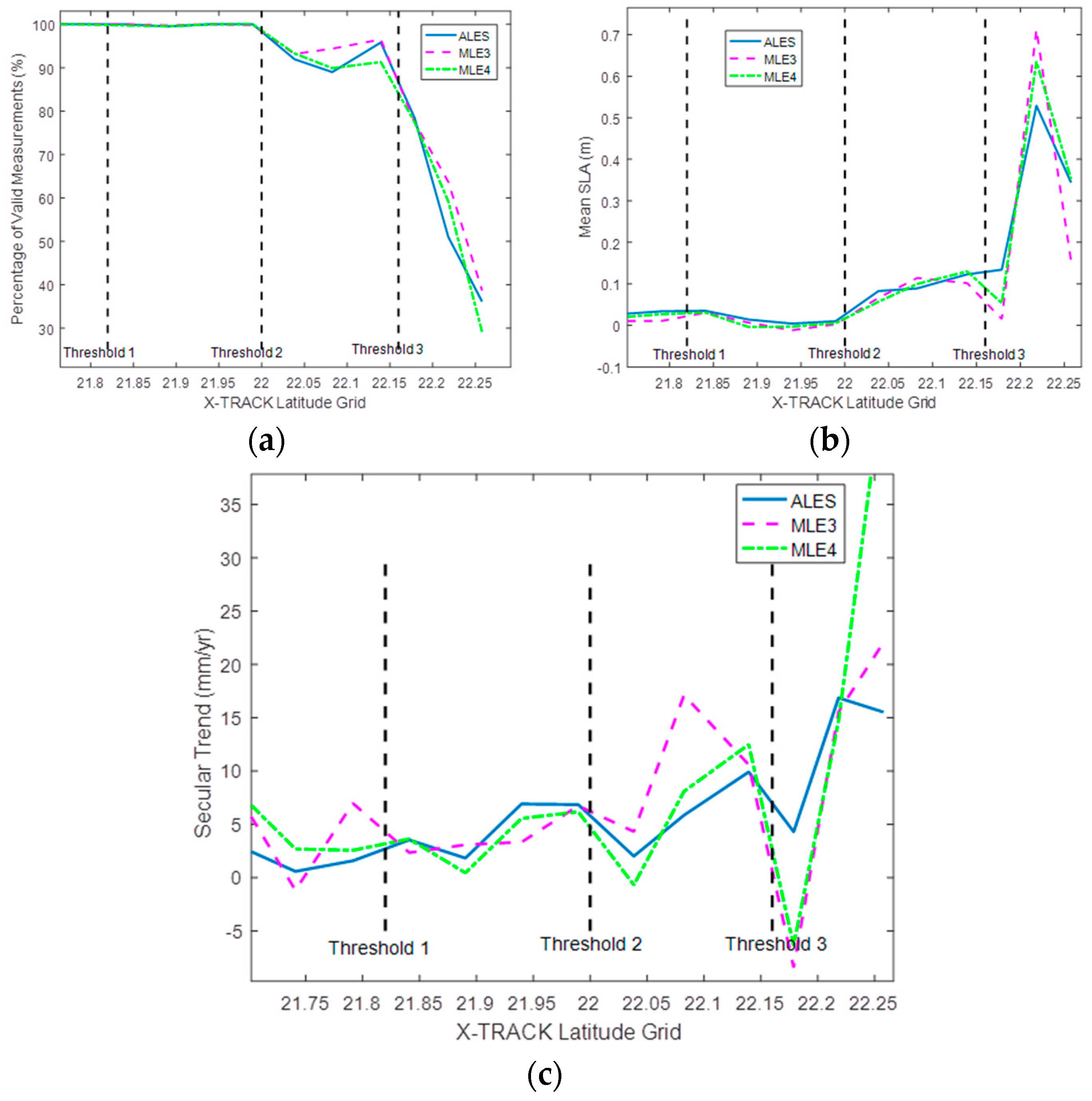
Here, we examine the relative performance of the MLE3, MLE4, and ALES retrackers in the H-Kcoastal zone. Because ALES and PISTACH are L2 products, we used the L3 X-TRACK product to project ALES and PISTACH MLE3 and MLE4 SLA onto regular 1-Hz reference points along the track, allowing us to obtain SLA time series over the study period. Figure 11a shows the percentage of valid measurements obtained for the different retrackers. MLE3 seems to be the most robust near the coast in the sense that it provides more valid data. Figure 11b shows the time-averaged SLA values for the three retrackers. Over the open ocean, ALES and MLE4 agree well (within 1 cm); MLE3 has a negative bias of 1–2 cm. Near the coast, ALES shows less variations, while MLE3 and MLE4 display large peaks likely due to retracking errors. Figure 11c shows the trend estimates for the different retrackers. ALES displays the smoothest pattern, which seems to indicate a better performance than MLE3 and MLE4.
The sea level residuals obtained after removing the trend and seasonal signal are shown in Figure 12 for MLE3, MLE4, ALES and the tide gauge data. A 3-month low pass filter was applied to the different SLA time series. For most cycles, the altimetry-based SLA have variations similar to the tide gauge, but the latter occasionally shows larger anomalies. In the first few cycles, the tide gauge residuals have surprising low values, and around cycle 135–160 have a few large negative peaks. Very local small-scale tides, waves, and currents may cause these sea level signals. The standard deviations of the altimetry SLA residuals with respect to the tide gauge residuals, before and after the 3-month smoothing, are given in Table 6. The improvement due to the smoothing is significant, the standard deviations decreasing by more than 50%. The consistency between the altimetry and tide gauge residuals is about 5 cm, which is encouraging given that the study area which is quite complex. ALES SLA has slightly larger standard deviation with respect to tide gauge sea level.
5.5. Impact of the Geophysical Corrections
As mentioned above, different solutions for some of the geophysical corrections are provided with the different coastal altimetry products. This is the case in particular for the wet tropospheric delay and ocean tides correction. In order to test their relative impact on the quality of the coastal altimetry sea level data, as well as to define the best choice of corrections, we use the different possibilities in Equation (1) to derive different sea level data sets (only one term varies in each case). Concerning the wet tropospheric correction, we tested both the decontaminated solution from the radiometer [26] and the composite correction derived from ECMWF and the radiometer. Concerning the tides, we considered both FES2004 and FES2012, besides GOT4.8. We also computed a version without the DAC. Given the results obtained above, we concentrated on case 1 area. Different diagnostics are considered to evaluate the impact of the correction choice:
Inspection of Table 6 and Table 7 indicates that the impact of the wet tropospheric correction is rather low. For the trend estimates, the uncertainties are the same but the composite wet delay results are +0.1–0.2 mm/yr larger. Some values of the standard deviations of the differences w.r.t the tide gauge data increase, but some others decrease.
The impact of the ocean tide correction appears much more important. The use of FES tide solutions introduces slightly less residual errors than GOT 4.8. FES2012 decreases the trend uncertainties, but the trend estimate seems too large (large difference with respect to the tide gauge). Correlations for different tide solutions with respect to the tide gauge data are also shown in Table 9. All ocean tide solutions lead to excellent correlations between altimetry-based and tide gauge-based sea level. FES 2012 gives the highest correlation, FES2004 the lowest.
Remember that we did not correct the HK tide gauge data from the DAC. Assuming that the tide gauge and altimeter roughly capture the same dynamic atmospheric effects, we should obtain better statistics if no DAC correction is applied to altimetry. It corresponds to what is observed in Table 8.
In conclusion, we note that the choice of the retracker and of the altimetry geophysical corrections, especially the tide correction, has a very significant impact on the estimated coastal sea level trend.
6. Discussion
There is a long-standing debate in the coastal altimetry community concerning the choice of the best retracking algorithms and still today, no consensus has emerged. From the results of this study, we consider that regarding the complexity of the corresponding radar echoes associated with the variety of existing coastal land surfaces, the choice of the retracker should be specific to the coastal area considered. We have however to keep in mind that this option does not suit for regional or global applications because we need homogeneous data sets, which would be difficult to obtain if one switches from one retracker to another as a function of the oceanic region considered. This would certainly produce bias in the estimated sea level.
Although the results obtained in this study with ALES in the HK coastal area are already encouraging, we believe that they could be further improved. For example, one of the most useful advances in altimeter waveform processing is the Singular Value Decomposition (SVD) approach proposed by Ollivier [39]. The idea of SVD is to eliminate the waveform components which are relative to the minor singular value, since those components probably arise from system noises rather than real ocean signals. Near the coast, the waveforms can be very different, so only the “Brown-like” waveforms were singled out (according to the “wf_class” parameter in the PISTACH product) to establish the waveform matrix. Results for cycle #100 are shown here as an arbitrary example. For cycle #100, there are 420 waveforms considered as ocean waveforms offshore HK, 342 of which are Brown-like. Therefore it is sufficient to carry out SVD processing. We tested two typical thresholds: 90% and 80%. The 20-Hz epoch noise characteristics are provided in Table 10 (the 1-Hz noise is roughly similar to the 20-Hz one). The measurements are split into two regions: far from the coast (shoreline distance >10 km) and near the coast (shoreline distance ≤10 km). For both regions, the epoch noises are significantly improved when using the SVD. The present study is somewhat preliminary since we have not computed nor analyzed the SLA performances after the SVD processing, but this strategy looks like a serious option to consider in the future for coastal altimetry processing.
7. Conclusions
In this paper, we attempted to compare for the first time the three most advanced coastal altimetry products for Jason-2 satellite altimetry: ALES, PISTACH, and XTRACK. The HK coastal zone was selected because it is the only candidate in the South China Sea with available hourly tide gauge data for comparison and validation. Besides, the HK coast presents extremely complex geomorphological and environmental conditions that lead to quite different waveforms. We considered six retrackers: MLE4, MLE3, ALES, ICE1, ICE3, and RED3, and computed Jason-2 sea level for each retracker over a 6.5-year time span (Jason-2 cycles 1–238). We generated a time series (cycle-by-cycle) for each sea level estimate in three cases, each covering different spatial scales. We found that case 1 is a good compromise between coherence and accuracy, and may represent the best sea level estimate at the HK coast. This is probably because, in the study zone, it contains more land-free areas than cases 2 and 3 much contaminated by the presence of small islands. An interesting outcome is that averaging along-track altimetry data over distances larger than 10 km provides better agreement with the tide gauge record than using only altimetry data very close to the coast.
ICE3 and RED3 retrackers show surprising large jumps (~+0.2 m) around cycle #150, that prevents further quantitative analysis. Data from other cycles need to be analyzed to determine whether these jumps result from a software bug (possibly different algorithm versions). A number of studies have shown that improved threshold retrackers sometimes outperform physically-based retrackers, so if any jump is always present, the data set needs to be corrected.
The results indicate that, in spite of the presence of large outliers in ALES (up to tens of meters), after outlier-editing, ALES performs better than MLE4 and MLE3, both in terms of noise level and uncertainty in the sea level trend estimate. We validated the coastal altimetry-based sea level by comparing with data from the HK tide gauge (located ~10 km away). Applying a 3-month smoothing, the standard deviation between the altimetry and tide gauge sea level time series is about 5 cm, which is quite encouraging given the complexity of the study area.
Another interesting result is that the computed sea level trend within 5 km from the coast is about twice the trend estimated at larger distances from the coast. This result, based on merging the CCI open ocean-based sea level with the retracked coastal data, suggests that offshore of the HK region, the short-term trend significantly increases when approaching the coast. This result cannot be generalized for several reasons, in particular because the estimated short-term trends essentially represent the inter-annual variability that may be different from one region to another.
Although the results presented here are encouraging, as shown in Section 6, the HK coastal altimetry sea level data could be further improved by applying an SVD processing before the waveform analysis. There is also certainly room to develop better altimeter waveform retrackers. Geophysical corrections, in particular tide corrections, also appear as an important limiting factor for coastal altimetry applications. In parallel, even if they provide much shorter time series of data than the TOPEX/Poseidon and -Jason missions, we could consider additional altimetry missions (such as HY-2A as well as SARAL/AltiKa and Sentinel-3 based respectively on Ka-band and delay-Doppler technology). In the near future, it will be also highly beneficial to systematically combine the best retrackers and geophysical corrections, to provide a coastal sea level data set with global coverage, usable for climate studies and coastal impact investigations.
Acknowledgments
This study is supported by the National Key R & D Program of China under contract #2017YFB0502800 and #2017YFB0502802, and by the Open Fund of State Key Laboratory of Remote Sensing Science (Grant No. OFSLRSS201705). We are very grateful to Fernando Nino for providing us with Figure 2. Xi-Yu Xu was funded by the China Scholarship Council (Grant No. 201604910329) during a one year visit in LEGOS. Jason-2 SGDR data are archived and maintained by AVISO. X-TRACK, ALES, and PISTACH data are generated and distributed by LEGOS/CTOH, NOC and CLS respectively. Special gratitude is also given to the three peer-reviewers, whose insightful comments have improved the manuscript significantly.
Author Contributions
Xi-Yu Xu collected and processed the coastal altimetry and CCI data and computed all results presented in the paper. Florence Birol processed the tide gauge data and checked the results. All three authors contributed to discuss the results and wrote the manuscript.
Conflicts of Interest
The authors declare no conflict of interest.
References
- Nicholls, R.J. Planning for the impacts of sea level rise. Oceanography 2011, 24, 144–157. [Google Scholar] [CrossRef]
- Brown, G. The average impulse response of a rough surface and its applications. IEEE Trans. Antennas Propag. 1977, 25, 67–74. [Google Scholar] [CrossRef]
- Passaro, M.; Cipollini, P.; Vignudelli, S.; Quartly, G.D.; Snaith, H.M. ALES: A multimission adaptive subwaveform retracker for coastal and open ocean altimetry. Remote Sens. Environ. 2014, 145, 173–189. [Google Scholar] [CrossRef] [Green Version]
- Cipollini, P.; Calafat, F.M.; Jevrejeva, S.; Melet, A.; Prandi, P. Monitoring sea level in the coastal zone with coastal altimetry and tide gauges. Surv. Geophys. 2017, 38, 33–57. [Google Scholar] [CrossRef]
- Cipollini, P.; Birol, F.; Fernandes, M.J.; Obligis, E.; Passaro, M.; Strub, P.T.; Valladeau, G.; Vignudelli, S.; Wilkin, J. Satellite altimetry in coastal regions. In Satellite Altimetry over Oceans and Land Surfaces; Stammer, D., Cazenave, A., Eds.; CRC Press: Boca Raton, FL, USA, 2017; ISBN 978-1-4987-4345. [Google Scholar]
- Birol, F.; Fuller, N.; Lyard, F.; Cancet, M.; Niño, F.; Delebecque, C.; Fleury, S.; Toublanc, F.; Melet, A.; Saraceno, M. Coastal applications from nadir altimetry: Example of the X-TRACK regional products. Adv. Space Res. 2017, 59, 936–953. [Google Scholar] [CrossRef]
- Vignudelli, S.; Kostianoy, A.G.; Cipollini, P.; Benveniste, J. (Eds.) Coastal Altimetry; Springer: Berlin/Heidelberg, Germany, 2011; 565p. [Google Scholar] [CrossRef]
- Mercier, F.; Rosmorduc, V.; Carrere, L.; Thibaut, P. Coastal and Hydrology Altimetry Product (PISTACH) Handbook; CLS-DOS-NT-10-246; CNES: Paris, France, 2010. [Google Scholar]
- Valladeau, G.; Thibaut, P.; Picard, B.; Poisson, J.C.; Tran, N.; Picot, N.; Guillot, A. Using SARAL/AltiKa to improve Ka-band altimeter measurements for coastal zones, hydrology and ice: The PEACHI prototype. Mar. Geodesy 2015, 38 (Suppl. 1), 124–142. [Google Scholar] [CrossRef]
- Caldwell, P.C.; Merrifield, M.A. Joint Archive for Sea Level Data Report; JIMAR Contribution No. 15-392, Data Report No. 24; University of Hawaii at Manoa, Joint Institute for Marine and Atmospheric Research: Manoa, HI, USA, 2015. [Google Scholar]
- Lai, W.S.; Matthew, J.P.; Ho, K.Y.; Astudillo, J.C.; Yung, M.N.; Russell, B.D.; Williams, G.A.; Leung, M.Y. Hong Kong’s marine environments: History, challenges and opportunities. Reg. Stud. Mar. Sci. 2016, 8, 259–273. [Google Scholar] [CrossRef]
- Gommenginger, C.; Thibaut, P.; Fenoglio-Marc, L.; Quartly, G.; Deng, X.; Gómez-Enri, J.; Challenor, P.; Gao, Y. Retracking Altimeter Waveforms Near the Coasts. In Coastal Altimetry; Vignudelli, S., Kostianoy, A., Cipollini, P., Benveniste, J., Eds.; Springer: Berlin/Heidelberg, Germany, 2011; pp. 61–101. [Google Scholar]
- Hwang, C.; Guo, J.; Deng, X.; Hsu, H.-Y.; Liu, Y. Coastal gravity anomalies from retracked Geosat/GM altimetry: Improvement, limitation and the role of airborne gravity data. J. Geodesy 2006, 80, 204–216. [Google Scholar] [CrossRef]
- Wingham, D.J.; Rapley, C.G.; Griffiths, H. New techniques in satellite tracking systems. In Proceedings of the IGARSS’86 Symposium, Zürich, Switzerland, 8–11 September 1986; pp. 1339–1344. [Google Scholar]
- Davis, C.H. Growth of the Greenland ice sheet: A performance assessment of altimeter retracking algorithms. IEEE Trans. Geosci. Remote Sens. 1995, 33, 1108–1116. [Google Scholar] [CrossRef]
- Mercier, F.; Picot, N.; Thibaut, P.; Cazenave, A.; Seyler, F.; Kosuth, P.; Bronner, E. CNES/PISTACH Project: An Innovative Approach to Get Better Measurements over in-Land Water Bodies from Satellite Altimetry: Early Results. In EGU General Assembly Conference Abstracts, Proceedings of the European Geosciences Union General Assembly 2009, Vienna, Austria, 19–24 April 2009; Copernicus Publications: Gettingen, Germany, 2009; Volume 11, p. 11674. [Google Scholar]
- Bao, L.; Lu, Y.; Wang, Y. Improved retracking algorithm for oceanic altimeter waveforms. Prog. Nat. Sci. 2009, 19, 195–203. [Google Scholar] [CrossRef]
- Yang, L.; Lin, M.; Liu, Q.; Pan, D. A coastal altimetry retracking strategy based on waveform classification and subwaveform extraction. Int. J. Remote Sens. 2012, 33, 7806–7819. [Google Scholar] [CrossRef]
- Chan, Y.W. Tide Reporting and Applications in Hong Kong, China. 2006. Available online: www.gloss-sealevel.org/publications/documents/hong_kong2006.pdf (accessed on 7 February 2018).
- Ablain, M.; Cazenave, A.; Larnicol, G.; Balmaseda, M.; Cipollini, P.; Faugère, Y.; Fernandes, M.J.; Henry, O.; Johannessen, J.A.; Knudsen, P.; et al. Improved sea level record over the satellite altimetry era (1993–2010) from the Climate Change Initiative project. Ocean Sci. 2015, 11, 67–82. [Google Scholar] [CrossRef] [Green Version]
- Ablain, M.; Legeais, J.F.; Prandi, P.; Marcos, M.; Fenoglio-Marc, L.; Dieng, H.B.; Benveniste, J.; Cazenave, A. Satellite altimetry-based sea level at global and regional scales. Surv. Geophys. 2017, 38, 7–31. [Google Scholar] [CrossRef]
- Legeais, J.F.; Ablain, M.; Zawadzki, L.; Zuo, H.; Johannessen, J.A.; Scharffenberg, M.G.; Fenoglio-Marc, L.; Fernandes, J.; Andersen, O.B.; Rudenko, S.; et al. An Accurate and Homogeneous Altimeter Sea Level Record from the ESA Climate Change Initiative, submitted. Earth Syst. Sci. Data 2017. [Google Scholar] [CrossRef]
- Thibaut, P.; Amarouche, L.; Zanife, L.O.Z.; Stunou, N.; Vincent, P.; Raizonville, P. Jason-1 altimeter ground processing look-up correction tables. Mar. Geodesy 2004, 27, 409–431. [Google Scholar] [CrossRef]
- Xu, X.Y.; Xu, K.; Wang, Z.Z.; Liu, H.G.; Wang, L. Compensating the PTR and LPF Features of the HY-2A Satellite Altimeter Utilizing Look-Up Tables. IEEE J. Sel. Top. Appl. Earth Obs. Remote Sens. 2015, 8, 149–159. [Google Scholar] [CrossRef]
- Dumont, J.P.; Rosmorduc, V.; Carrere, L.; Picot, N.; Bronner, E.; Couhert, A.; Desai, S.; Bpnekamp, H.; Scharroo, R.; Lillibridge, J. OSTM/Jason-2 Products Handbook (Issue: 1 rev 11). SALP-MU-M-OP-15815-CN. 2017. Available online: https://www.aviso.altimetry.fr/fileadmin/documents/data/tools/hdbk_j2.pdf (accessed on 7 February 2018).
- Brown, S. A Novel Near-Land Radiometer Wet Path-Delay Retrieval Algorithm: Application to the Jason-2/OSTM Advanced Microwave Radiometer. IEEE Trans. Geosci. Remote Sens. 2010, 48, 1986–1992. [Google Scholar] [CrossRef]
- Fernandes, M.J.; Lázaro, C.; Ablain, M.; Pires, N. Improved wet path delays for all ESA and reference altimetric missions. Remote Sens. Environ. 2015, 169, 50–74. [Google Scholar] [CrossRef]
- Ray, R.D.; Egbert, G.D.; Erofeeva, S.Y. Tide predictions in shelf and coastal waters: Status and prospects. In Coastal Altimetry; Vignudelli, S., Kostianoy, A.G., Cipollini, P., Benveniste, J., Eds.; Springer: Berlin/Heidelberg, Germany, 2011; Chapter 7. [Google Scholar]
- Lyard, F.; Lefevre, F.; Letellier, T.; Francis, O. Modelling the global ocean tides: Modern insights from FES2004. Ocean Dyn. 2006, 56, 394–415. [Google Scholar] [CrossRef]
- Ray, R. Status of Modeling Shallow-water Ocean Tides: Report from Stammer international model comparison project. In Proceedings of the NASA/CNES Surface Water and Ocean Topography (SWOT) Science Definition Team (SDT) Meeting, Toulouse, France, 26–28 June 2014. [Google Scholar]
- Glover, D.M.; Jenkins, W.J.; Doney, S.C. Modeling Methods for Marine Science; Cambridge University Press: Cambridge, UK, 2011; 571p. [Google Scholar]
- Masters, D.; Nerem, R.S.; Choe, C.; Leuliette, E.; Beckley, B.; White, N.; Ablain, M. Comparison of global mean sea level time series from TOPEX/Poseidon, Jason-1, and Jason-2. Mar. Geodesy 2012, 35, 20–41. [Google Scholar] [CrossRef]
- Chambers, D.P.; Cazenave, A.; Champollion, N.; Dieng, H.; Llovel, W.; Forsberg, R.; Schuckmann, K.; Wada, Y. Evaluation of the Global Mean Sea Level Budget between 1993 and 2014. Surv. Geophys. 2017, 38, 309–327. [Google Scholar] [CrossRef]
- Xu, X.Y.; Liu, H.G.; Yang, S.B. Echo phase characteristic of interferometric altimeter for case of random surface plus one strong point scatter. In Proceedings of the 2016 IEEE International Geoscience and Remote Sensing Symposium (IGARSS), Beijing, China, 10–15 July 2016; pp. 6456–6459. [Google Scholar]
- Halimi, A.; Mailhes, C.; Tourneret, J.-Y.; Thibaut, P.; Boy, F. Parameter estimation for peaky altimetric waveforms. IEEE Trans. Geosci. Remote Sens. 2013, 51, 1568–1577. [Google Scholar] [CrossRef] [Green Version]
- Cazenave, A.; Dominh, K.; Ponchaut, F.; Soudarin, L.; Crétaux, J.F.; Le Provost, C. Sea level changes from Topex-Poseidon altimetry and tide gauges, and vertical crustal motions from DORIS. Geophys. Res. Lett. 1999, 26, 2077–2080. [Google Scholar] [CrossRef]
- Yuan, L.G.; Ding, X.L.; Chen, W.; Guo, Z.H.; Chen, S.B.; Hong, B.S.; Zhou, J.T. Characteristics of daily position time series from the Hong Kong GPS fiducial network. Chin. J. Geophys. 2008, 51, 1372–1384. [Google Scholar] [CrossRef]
- Lau, D.S.; Wong, W.T. Monitoring Crustal Movement in Hong Kong Using GPS: Preliminary Results; Hong Kong Observatory: Hong Kong, China, 2010. [Google Scholar]
- Ollivier, A. Nouvelle Approche Pour L’extraction de Paramtres Gophysiques Partir Des Mesures en Altimtrie Radar. Ph.D. Thesis, Institut National Polytechnique de Grenoble, Grenoble, France, 2006. [Google Scholar]
Figure 1.
Examples of typical open ocean waveform (left; the red line corresponds to the fitted Brown model) and coastal ocean waveform (right).
Figure 1.
Examples of typical open ocean waveform (left; the red line corresponds to the fitted Brown model) and coastal ocean waveform (right).

Figure 2.
Map showing the study area, the selected Jason-2 pass 153 (black and colored line) and the Quarry Bay tide gauge (red circle). The latter is located ~10 km away from the Jason-2 pass. The along-track sections corresponding to study cases 1, 2, and 3 are also indicated (orange, green, and blue-green dashed lines, respectively). The background map is from Google Earth.

Figure 3.
Bathymetry and shoreline distance at the Hong-Kong (HK) coast along 3 segments of the Jason-2 pass identified as cases 1, 2, and 3 (see location in Figure 2).
Figure 3.
Bathymetry and shoreline distance at the Hong-Kong (HK) coast along 3 segments of the Jason-2 pass identified as cases 1, 2, and 3 (see location in Figure 2).

Figure 4.
HK tide gauge sea level time series (in meters) interpolated to Jason-2 observations.

Figure 5.
Sea state bias (SSB) difference with respect to Significant Wave Height.

Figure 6.
20-Hz sea level anomaly (SLA) before (left) and after (right) editing. Jason-2 cycle 5 is considered here.
Figure 6.
20-Hz sea level anomaly (SLA) before (left) and after (right) editing. Jason-2 cycle 5 is considered here.

Figure 7.
Percentages of waveform categories in the 3 cases.

Figure 8.
Regional 6.5 yr-long trends in sea level derived from the CCI sea level data. (a) using gridded data and (b) interpolated along the Jason-2 pass 153. Vertical blue bars in Figure 8b represent the uncertainty on the trend estimation.
Figure 8.
Regional 6.5 yr-long trends in sea level derived from the CCI sea level data. (a) using gridded data and (b) interpolated along the Jason-2 pass 153. Vertical blue bars in Figure 8b represent the uncertainty on the trend estimation.


Figure 9.
Regional 6.5 yr-long trends in sea level derived from filtered X-TRACK data along the Jason-2 pass 153. Vertical blue bars represent the uncertainty on the trend estimation.
Figure 9.
Regional 6.5 yr-long trends in sea level derived from filtered X-TRACK data along the Jason-2 pass 153. Vertical blue bars represent the uncertainty on the trend estimation.

Figure 10.
SLA means and noise levels. (a) Case 1, mean SLA for ALES, MLE3 and MLE4; (b) Case 2, mean SLA for ALES, MLE3 and MLE4; (c) Case 3, mean SLA for ALES, MLE3 and MLE4; (d) Case 1, mean SLA for ICE1, ICE3 and RED3; (e) Case 2, mean SLA for ICE1, ICE3 and RED3; (f) Case 3, mean SLA for ICE1, ICE3 and RED3; (g) Case 1, noise levels for ALES, MLE3 and MLE4; (h) Case 2, noise levels for ALES, MLE3 and MLE4; (i) Case 3, noise levels for ALES, MLE3 and MLE4; (j) Case 1, noise levels for ICE1, ICE3 and RED3; (k) Case 2, noise levels for ICE1, ICE3 and RED3; (l) Case 3, noise levels for ICE1, ICE3 and RED3.


Figure 11.
(a) Percentage of valid measurements; (b,c) mean values and 6.5-yr trend estimates for ALES, MLE3, and MLE4 retrackers. Results are presented as a function of latitude.
Figure 11.
(a) Percentage of valid measurements; (b,c) mean values and 6.5-yr trend estimates for ALES, MLE3, and MLE4 retrackers. Results are presented as a function of latitude.

Figure 12.
Detrended and deseasoned SLA time series based on ALES, MLE3, and MLE4, with 3-month smoothing (tide gauge SLA—noted TG—is shown as reference).
Figure 12.
Detrended and deseasoned SLA time series based on ALES, MLE3, and MLE4, with 3-month smoothing (tide gauge SLA—noted TG—is shown as reference).


Table 1.
Overview of different retrackers applied in different altimetry products.
| Retracker | Product | Idea | Sub-Waveform | Comments |
|---|---|---|---|---|
| MLE4 | SGDR 1 | Brown model | No | Official standard retracker. |
| MLE3 | SGDR 1 | Brown model | No | |
| OCE3 | PISTACH | Brown model | No | Same as MLE3 |
| RED3 | PISTACH | Brown model | Fixed: bins: t0 + [−10:20] | Simplified version of ALES |
| ALES | ALES | Brown model | Adaptive to the SWH | Two-pass retracker |
| ICE1 | PISTACH | Modified threshold | No | |
| ICE3 | PISTACH | Modified threshold | Fixed: bins: t0 + [−10:20] |
1: SGDR contains all GDR parameters, plus some supplementary items such as the retracker outputs and waveforms.
Table 2.
Overview of the five categories defined from the 16 PISTACH classes.
| Category | Waveform Characteristics | Possible Surface Observed | Retracking Strategy |
|---|---|---|---|
| Brown | The waveform is close to the Brown model. | The land contribution in the altimeter footprint is null or small. | MLE4 |
| Distorted Brown | The waveform is similar to the Brown model, but with distortions (either with an increasing plateau, or with a sharply decreasing plateau, or with a too broad noise floor). | There is land signature at the fringe of the altimeter footprint, with different reflection than over open ocean surface. | ALES |
| Peak dominated | One (or a few) large peak(s) dominate(s) the waveform; there may be a Brown shape in the waveform, but its maximum power is much lower than the peak(s). | There are one or a few strong bright targets (e.g., extremely calm water surface or effective corner reflector, see [34]) within the altimeter footprint. | MLE based on Gaussian model or improved threshold |
| Brown + Peak | The waveform is a mixture of Brown shape and one (or a few) peak(s) with comparable power levels. The location of the peak can be in the leading edge or the plateau. | The portions of ocean and land surfaces within the altimeter footprint are equivalent. | MLE based on BAGP (Brown with Asymmetric Gaussian Peak [35]) |
| Others | Unexplained waveform patterns (e.g., very noisy echoes or linear echoes). | Unexplainable surface features (e.g., very composite geomorphology or some extreme events). | Should be rejected. |
Table 3.
Estimated linear trend and associated uncertainty (mm/yr) as a function of sea level data source and case.
Table 3.
Estimated linear trend and associated uncertainty (mm/yr) as a function of sea level data source and case.
| Data Source | Case 1 | Case 2 | Case 3 |
|---|---|---|---|
| ALES | +5.9 ± 1.5 | +9.7 ± 1.6 | +17.3 ± 2.3 |
| MLE3 | +5.0 ± 1.6 | +8.1 ± 2.2 | +2.6 ± 3.1 |
| MLE4 | +4.2 ± 1.6 | +4.3 ± 2.2 | +5.5 ± 3.5 |
| ICE1 | −29.1 ± 2.4 | −27.5 ± 2.8 | −22.9 ± 4.0 |
| ICE3 | +57.5 ± 2.3 | +60.1 ± 2.5 | +52.9 ± 3.0 |
| RED3 | +55.3 ± 2.1 | +58.0 ± 2.3 | +58.5 ± 3.0 |
| XTRACK | +8.6 ± 2.2 | ||
| Tide Gauge (in-situ reference) | +5.2 ± 2.0 | ||
| Tide Gauge (After VLM correction) | +5.5 ± 2.0 | ||
| Regional trend from the CCI data | 2.7 ± 2.0 | ||
Table 4.
Estimated annual amplitude (cm) and phase (degree) as a function of sea level data source and case.
Table 4.
Estimated annual amplitude (cm) and phase (degree) as a function of sea level data source and case.
| Data Source | Case 1 | Case 2 | Case 3 |
|---|---|---|---|
| ALES | 13.05/344 | 12.49/348 | 11.19/2 |
| MLE3 | 13.29/338 | 12.39/339 | 13.17/343 |
| MLE4 | 12.96/339 | 11.44/340 | 11.12/348 |
| XTRACK | 13.23/338 | ||
| Tide Gauge | 11.46/311 | ||
Table 5.
Estimated semiannual amplitude (cm) and phase (degree) as a function of sea level data source and case.
Table 5.
Estimated semiannual amplitude (cm) and phase (degree) as a function of sea level data source and case.
| Data Source | Case 1 | Case 2 | Case 3 |
|---|---|---|---|
| ALES | 6.03/235 | 5.67/239 | 7.38/260 |
| MLE3 | 6.17/241 | 6.76/252 | 9.24/270 |
| MLE4 | 6.02/236 | 6.96/245 | 11.80/262 |
| XTRACK | 6.81/223 | ||
| Tide Gauge | 7.62/236 | ||
Table 6.
Deseasoned and detrended SLA standard deviation w.r.t. tide gauge sea level (cm) for case 1.
Table 6.
Deseasoned and detrended SLA standard deviation w.r.t. tide gauge sea level (cm) for case 1.
| SLA Series | ALES | MLE3 | MLE4 |
|---|---|---|---|
| Agreement | 5.12 | 4.82 | 4.88 |
Table 7.
Secular trend and associated uncertainty (mm/yr) for case 1, with different geophysical corrections choices. DAC = dynamic atmospheric correction.
Table 7.
Secular trend and associated uncertainty (mm/yr) for case 1, with different geophysical corrections choices. DAC = dynamic atmospheric correction.
| Choice | ALES | MLE3 | MLE4 |
|---|---|---|---|
| Standard choice (Table 4) | +5.9 ± 1.5 | +5.0 ± 1.6 | +4.2 ± 1.6 |
| composite wet delay | +6.1 ± 1.5 | +5.1 ± 1.6 | +4.3 ± 1.6 |
| FES 2004 ocean tide | +5.7 ± 1.5 | +4.6 ± 1.6 | +4.7 ± 1.6 |
| FES 2012 ocean tide | +9.1 ± 1.3 | +7.8 ± 1.5 | +7.1 ± 1.5 |
| No DAC applied | +6.3 ± 1.6 | +5.1 ± 1.8 | +4.5 ± 1.7 |
Table 8.
Residual SLA, standard deviation w.r.t. tide gauge-based sea level (cm), for case 1, after 3-month smoothing, with different geophysical corrections choices.
Table 8.
Residual SLA, standard deviation w.r.t. tide gauge-based sea level (cm), for case 1, after 3-month smoothing, with different geophysical corrections choices.
| Choice | ALES | MLE3 | MLE4 |
|---|---|---|---|
| Standard choice (Table 4) | 5.12 | 4.82 | 4.88 |
| composite wet delay | 5.02 | 4.80 | 5.01 |
| FES 2004 ocean tide | 4.87 | 4.76 | 4.82 |
| FES 2012 ocean tide | 4.89 | 4.56 | 4.88 |
| No DAC applied | 4.84 | 4.56 | 4.76 |
Table 9.
Correlations of different tide solutions with respect to the tide gauge tide height.
| Ocean Tide Solution | GOT 4.8 | FES 2004 | FES 2012 |
|---|---|---|---|
| Correlation | 0.91 | 0.89 | 0.95 |
Table 10.
20-Hz epoch noise (cm) for different singular value decomposition (SVD) configurations (cycle #100).
Table 10.
20-Hz epoch noise (cm) for different singular value decomposition (SVD) configurations (cycle #100).
| Threshold Percentage | No SVD | 90% SVD | 80% SVD |
|---|---|---|---|
| Far from the coast | 8.66 | 8.05 | 7.52 |
| Near the coast | 9.41 | 8.90 | 8.60 |
| The last ocean-like waveform | 39.17 | 36.18 | 34.68 |
© 2018 by the authors. Licensee MDPI, Basel, Switzerland. This article is an open access article distributed under the terms and conditions of the Creative Commons Attribution (CC BY) license (http://creativecommons.org/licenses/by/4.0/).
Share and Cite
MDPI and ACS Style
Xu, X.-Y.; Birol, F.; Cazenave, A. Evaluation of Coastal Sea Level Offshore Hong Kong from Jason-2 Altimetry. Remote Sens. 2018, 10, 282. https://doi.org/10.3390/rs10020282
AMA Style
Xu X-Y, Birol F, Cazenave A. Evaluation of Coastal Sea Level Offshore Hong Kong from Jason-2 Altimetry. Remote Sensing. 2018; 10(2):282. https://doi.org/10.3390/rs10020282
Chicago/Turabian StyleXu, Xi-Yu, Florence Birol, and Anny Cazenave. 2018. "Evaluation of Coastal Sea Level Offshore Hong Kong from Jason-2 Altimetry" Remote Sensing 10, no. 2: 282. https://doi.org/10.3390/rs10020282
Note that from the first issue of 2016, this journal uses article numbers instead of page numbers. See further details here.