Multiscale Geoscene Segmentation for Extracting Urban Functional Zones from VHR Satellite Images


1
Institute of Remote Sensing and GIS, Peking University, Beijing 100871, China
2
Satellite Environment Center, Ministry of Environmental Protection, Beijing 100094, China
3
State Key Laboratory of Urban and Regional Ecology, Research center for Eco-Environmental Sciences, Chinese Academy of Sciences, Beijing 100085, China
*
Author to whom correspondence should be addressed.
Remote Sens. 2018, 10(2), 281; https://doi.org/10.3390/rs10020281
Submission received: 28 December 2017
/
Revised: 30 January 2018
/
Accepted: 8 February 2018
/
Published: 12 February 2018
Abstract
:Urban functional zones, such as commercial, residential, and industrial zones, are basic units of urban planning, and play an important role in monitoring urbanization. However, historical functional-zone maps are rarely available for cities in developing countries, as traditional urban investigations focus on geographic objects rather than functional zones. Recent studies have sought to extract functional zones automatically from very-high-resolution (VHR) satellite images, and they mainly concentrate on classification techniques, but ignore zone segmentation which delineates functional-zone boundaries and is fundamental to functional-zone analysis. To resolve the issue, this study presents a novel segmentation method, geoscene segmentation, which can identify functional zones at multiple scales by aggregating diverse urban objects considering their features and spatial patterns. In experiments, we applied this method to three Chinese cities—Beijing, Putian, and Zhuhai—and generated detailed functional-zone maps with diverse functional categories. These experimental results indicate our method effectively delineates urban functional zones with VHR imagery; different categories of functional zones extracted by using different scale parameters; and spatial patterns that are more important than the features of individual objects in extracting functional zones. Accordingly, the presented multiscale geoscene segmentation method is important for urban-functional-zone analysis, and can provide valuable data for city planners.
1. Introduction
1.1. Background
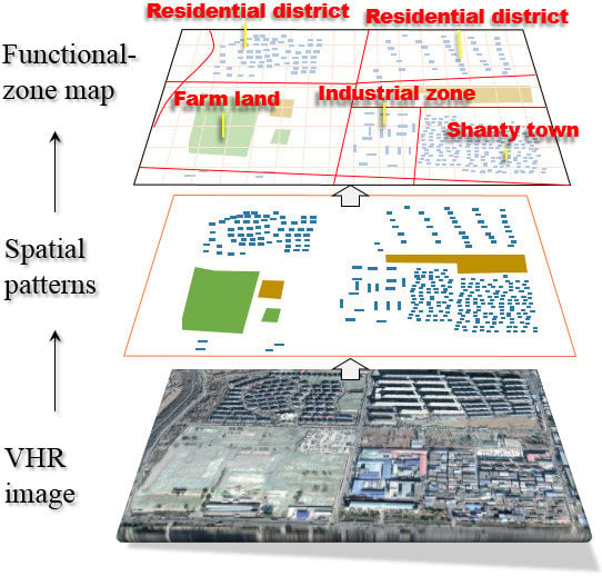
Urban functional zones are basic units of urban planning and management [1,2], categorizing where people undertake different socioeconomic activities [3]. In most cities, they consist of commercial zones, residential districts, industrial zones, shanty towns, and parks (Figure 1). Essentially, functional zones are spatially aggregated into regular patterns of diverse geographic objects, and their categories are semantically abstracted from these objects’ land-use classes [4].
Originated in the 2000s, functional-zone analysis is a technique of studying the relationship between urban landscapes and human activities [5]. The past ten years have witnessed its rapid development, owing to the improvement of remotely sensed images, especially very-high-resolution (VHR) ones, with which more detailed information on functional zones can be gleaned than ever before [6,7]. Zhang et al. (2015) proposed that the functional-zone analysis was composed of three steps [8], i.e., zone segmentation, feature representation, and function classification (Figure 2). Firstly, functional zones are spatially delineated within original VHR images using zone segmentation. Then, multiple features are extracted to characterize each functional zone. Finally, functional zones can be labeled with categories based on their features. Previous efforts at functional-zone analysis focus mainly on feature representations [9,10,11,12,13,14] and classification methods [4,15,16], but ignore zone segmentation. This is unfortunate because zone segmentation is an essential precursor to the other two steps of functional-zone analysis and is hence fundamental to the entire undertaking.
Existing image segmentation methods [9,17,18] are designed to extract homogeneous objects with consistent spectrums and regular shapes [19,20,21], but cannot delineate functional zones with high heterogeneities and substantial discontinuities in visual cues [22,23]. Considering the complexity and heterogeneity of functional zones, Heiden et al. (2012) first proposed using road blocks to extract functional zones [24]. They utilized roads as boundaries to segment VHR satellite images into blocks which were regarded as functional zones. However, this method will be ineffective in the following three cases: (1) when the segmented blocks contain different kinds of functional zones [25], so a block does not fall entirely within an individual functional zone; (2) when there are temporal differences between VHR images and the used road data [26]; and (3) when researchers are seeking functional zones at a scale other than that of the blocks. Functional zones usually have different sizes and heterogeneities, which should be derived from segmentation results at multiple scales [27]. Accordingly, there is ample room for improvement on existing methods for generating functional zones from VHR satellite images [28].
1.2. Geoscene: Representation of Urban Functional Zones
Why are functional zones difficult to segment from VHR images? The reason is that pixels and even individual objects are inadequate to represent functional zones. In other words, the definitions of pixels and objects do not match those of functional zones, leading to neither pixels nor objects representing functional zones (Table 1). For example, a pixel in Figure 3a is an imaging unit of a sensor which represents the building material on a residential structure; the object in Figure 3b is a relatively homogeneous image patch representing a geographic object, in this case a residential building; and the “residential district” in Figure 3c is much more heterogeneous consisting of diverse objects such as buildings and roads. Accordingly, we need a novel unit other than pixels or objects to represent functional zones, such as that in Figure 3c. We name this unit a “geoscene”. Geoscenes refer to continuous regions in remote sensing images that do not overlap with each other. Specifically, each geoscene should comprise consistent spatial patterns, in which the same-category objects have similar object features and pattern characteristics.
Geoscenes can represent functional zones in the following three aspects. First, both comprise similar components. Functional zones are spatially composed of geographic objects, while geoscenes composed of image objects which can represent geographic ones. Second, they have the same feature representations. Both functional zones and geoscenes can be characterized by spatial patterns. Third, they are both impacted by scale parameters. For example, the sizes of geoscenes are directly dominated by segmentation scale, while those of functional zones can be impacted by the granularity of urban investigations; thus, multiscale geoscenes can be a potential way for different-granularity investigations of functional zones. Accordingly, geoscenes can represent functional zones from the three perspectives.
1.3. Technical Issues
To extract geoscenes from VHR images to represent functional zones, several technical issues should be considered, including feature representation, segmentation method, scale parameter, and evaluation. The relevant work on these topics is demonstrated as follows.
- Feature representation: Features are basic cues to segment and recognize functional zones, which can be divided into three levels: low, middle and high. Firstly, low-level features, such as spectral, geometrical, and textural image features, are widely used in image analyses [11], but they are weak in characterizing functional zones which are usually composed of diverse objects with variant characteristics [12]. Then, middle-level features, including object semantics [4,8], visual elements [7], and bag-of-visual-word (BOVW) representations [13], are more effective than low-level features in representing functional zones [7], but they ignore spatial and contextual information of objects, leading to inaccurate recognition results. To resolve this issue, Hu et al. (2015) extracted high-level features using convolutional neural network (CNN) [10], which could measure contextual information and were more robust than visual features in recognizing functional zones [14,16]. Zhang et al. (2017) had a different opinion on the relevance of deep-learning features and stated that these features rarely had geographic meaning and were weak for the purpose of interpretability [4]. Additionally, the size and shape of the convolution window can influence deep-learning features. Recently, spatial-pattern features measuring spatial object distributions are proposed to characterize functional zones and produce satisfactory classification results [4]. However, these spatial-pattern features are measured based on roads blocks which cannot necessarily be applied to zone segmentation [36]. Accordingly, the application of spatial-pattern features for functional-zone segmentation needs further studies.
- Segmentation method: Functional-zone segmentation aims to spatially divide an image into non-overlapping patches with each representing a functional zone. This is the first and fundamental step to functional-zone analysis. Existing segmentation methods can be sorted into three types: region, edge, and graph based [9,17,18]. Among them, a region-based method named multiresolution segmentation (MRS) outperforms others and is widely used for geographic-object-based analysis (GEOBIA) [18,37]. MRS essentially aggregates neighboring pixels into homogeneous objects by considering their spectral and shape heterogeneities. It concentrates on different kinds of geographic objects which should be segmented at multiple scales [38]. However, neither MRS nor other segmentation techniques can extract functional zones, as they focus on homogeneous objects which have consistent visual cues, but functional zones have substantial discontinuities in visual cues and can be divided into many smaller segments. Accordingly, functional-zone segmentation methods are still open and will be the focus of this study.
- Scale parameter: Scale is important for segmentation regarding tolerable heterogeneities of segmented functional zones. It influences segmentation results [18] and controls the sizes of segments. The used scales in existing segmentations can fall into two types, i.e., fixed and multiple [19,20,21,37]. Multiple scales will be more applicable to functional-zone segmentation, as functional zones are often different in sizes and heterogeneities, which are related to variant scale parameters. Accordingly, how to select the appropriate scales for functional-zone segmentations is one of the key issues in this study.
- Result evaluation: Evaluation aims to measure accuracies of segmentation results and verify the effectiveness of segmentation methods. Existing studies on segmentations consider two kinds of evaluation approaches, i.e., supervised and unsupervised evaluations [39,40,41]. For the supervised evaluation, the ground truths of functional-zone boundaries are required. The differences between ground truths and segmentation results are used to measure segmentation errors [19]. However, the ground truths of functional zones are rarely available, thus it is not applicative to use traditional supervised evaluations here. On the other hand, unsupervised evaluation is rooted in the idea of comparing within-segment heterogeneity to between-segment similarity [40], but functional zones are typically heterogeneous; thus, unsupervised evaluation is ineffective. Accordingly, neither method is applicable to the evaluation of functional-zone segmentations, thus a novel evaluation method should be further developed.
In summary, the four technical issues referred to above are critical to extracting functional zones, but they have yet to be resolved. This study aims to determine the solutions to the four issues, and extract functional zones from VHR satellite images. Four contributions are made in this research: (1) spatial-pattern features characterizing local spatial patterns of objects are proposed and used for functional-zone segmentation; (2) a geoscene segmentation method is first proposed to delineate functional zones at multiple scales; (3) two parameters, i.e., scale and the weight of spatial-pattern features, as well as their impacts on segmentation results are evaluated and reviewed; and (4) the proposed methods are used to map functional zones for three cities and compare their functional structures. The four contributions are novel and crucial to urban functional-zone analysis. To the best of our knowledge, this study is the first work on automatic functional-zone segmentation. Additionally, the terminologies presented in this study are outlined in Table 2.
2. Methodology
Aiming at resolving the four technical issues including feature representation, segmentation method, scale selection, and result evaluation, the methodology section consists of four parts (Figure 4). Firstly, spatial-pattern features are extracted to characterize the spatial arrangements of diverse objects, where the objects are generated by classical GEOBIA methods [42], as they are spatially delineated with multiresolution segmentations [19] and semantically labeled by support vector machine [43]. Secondly, a geoscene segmentation method is presented to extract functional zones. It aggregates different kinds of objects at different levels, and then overlays the multi-level object clusters to generate geoscenes. Thirdly, different scale parameters are used for geoscene segmentations, resulting in multiscale segmentation results which are organized with a hierarchical structure. Finally, multiscale segmentation results are evaluated based on the points-of-interest.
2.1. Spatial-Pattern Features
Both object and spatial-pattern features are considered in defining geoscenes. Object features which have been widely used in geographic-object-based image analysis [42], are mainly composed of spectral, geometrical, and textural features. In this study, spectral features are derived from spectral histograms of objects, which include average spectrums, standard deviations, and skewness of spectral histograms; textural features are extracted from gray-level co-occurrence matrix (GLCM), and contain homogeneity, dissimilarity, entropy, and correlation; and geometrical features characterize objects’ areas, shapes indexes, and main directions. The three kinds of features are capable of characterizing objects from different aspects [4]. On the other hand, spatial-pattern features measuring spatial object relations are inadequate [44], and therefore, this study concentrates on the spatial-pattern features and presents two kinds of measurements characterizing neighboring and disjoint relations between objects.
2.1.1. Spatial-Pattern Features of Neighboring Objects
In previous studies, common boundary information was measured to characterize neighboring relations between objects [8]. However, this kind of measurement ignores the sequence and features of surrounding objects, which are also important for characterizing spatial object patterns. In addition, the number of neighbors varies from object to object, so that it is difficult to measure neighboring relations in a unified way. To resolve these issues, a novel spatial-pattern feature is proposed.
Taking an object as an example (Figure 5), it has topologically neighboring objects, with representing its -th neighboring object (). The common boundary between and is denoted as , thus ’s boundary . In addition, represents the object features of (a vector containing spectral, geometrical, and textural features), and represents the dimension of object features. Accordingly, a matrix of size (Figure 6) can be generated to measure the spatial pattern in ’s neighborhood, where is a constant parameter which can restrict the to be a unified measurement for every object no matter how many neighbors it has.
measures three kinds of information including neighbors’ sequence, object features, and common boundary lengths. First, is composed of the object features, with each element being a feature value of a neighboring object. Then, common boundaries between and its neighbors are considered. The neighbor with a longer common boundary occupies more elements of , where is copied times to build the (Figure 6). Third, the sequence of ’s neighbors is also measured. is represented as a sequence, i.e., . For every object no matter how many neighbors it has, a matrix of can be extracted to characterize its neighboring spatial patterns, which considers object features, common boundaries, and sequence of neighbors. Accordingly, the proposed neighboring-spatial-pattern feature can comprehensively measure topologically neighboring relations between objects in a unified way.
2.1.2. Spatial-Pattern Features of Disjoint Objects
The spatial-pattern feature presented above characterizes the relations between topologically neighboring objects, but cannot measure the relations between disjoint objects. Accordingly, this section proposes another kind of spatial-pattern feature which measures disjoint relations by considering distances and directions.
-order neighbors are considered in measuring disjoint-spatial-pattern features. -order neighbors of object refer to the objects which are disjoint with but within a -order searching field. Here, disjoint-spatial-pattern features are measured per category. Supposing that categories of objects are concerned in total, and the -th category is represented as . For , its minimum distance to is represented as , its average distance to represented as , and the most frequent direction from to represented as . Accordingly, for each object, three features, i.e., , , and can be extracted to characterize their disjoint spatial patterns.
The two kinds of spatial-pattern features characterize the relations between neighboring and disjoint objects respectively, which can be combined together and spread into a super feature vector. The neighboring-spatial-pattern feature is a matrix, and the disjoint one is composed of three -dimension vectors. Accordingly, spatial-pattern features are extracted to characterize local spatial patterns.
2.2. Geoscene Segmentation
Geoscene segmentation is proposed to delineate functional zones in cities. It mainly consists of three steps, i.e., aggregation, expanding, and overlaying (Figure 7). First, land-cover objects generated by GEOBIA are organized into multi-level relationship networks. At each level, a relationship graph is established to measure the connections among one category of objects, and these objects will be aggregated based on the relationship graph by considering their similarities in object features and spatial patterns. However, the aggregated object clusters are discontinuous and interrupted by the other-category objects. Accordingly, these object clusters are spatially expanded in the second step. Finally, the multi-level clusters are overlaid together, and their common parts are output as geoscenes. The pseudocode of the geoscene segmentation is presented in Appendix A.
2.2.1. Aggregation
According to the definition of geoscene, the same-category objects within a geoscene should be similar in individual features and spatial patterns. Accordingly, the same-category objects are employed as the basic units for aggregation. In practice, objects of the same category are organized at one level, and diverse categories correspond to multiple levels.
Aggregation is conducted based on a relationship graph, where objects are denoted by nodes and their relations are represented by edges, and only the connected objects can be aggregated. Here, the connection is defined as follows: taking two objects, and , as examples, if the two objects belong to the same category and is within the -order neighborhood of , they can have a connection and should be linked by an edge. Accordingly, for each category of objects, a relationship graph can be established at a certain level. Based on the relationship graph (Figure 7), objects with similar features and spatial patterns will be aggregated.
The aggregation algorithm is proposed based on fractal net evolution theory [45]. Supposing that two object clusters and (Figure 8) are considered to be aggregated, their discrepancy is used as the indicator which is denoted by (Equation (1)) and measures the change in heterogeneity considering a virtual merging.
where represents the merged result which combines and . refers to the number of objects in , is the number of objects in , and . denotes the heterogeneity of , of , and of . These heterogeneities can be measured by the standard deviations of features, where both object and spatial-pattern features are considered (Equation (2)).
where represents the weight of spatial-pattern features. refers to the standard deviation of object features in , and is the standard deviation of spatial-pattern features in . They can be calculated by Equations (3) and (4) respectively.
where refers to the dimension of object features, denotes the -th object feature value of -th object in , and represents the mean value of -th object feature which is a scalar. Similarly, is the -th spatial-pattern characteristic of -th object in , represents the mean value of -th object feature, and refers to the dimension of spatial-pattern features.
Accordingly, can be calculated based on Equations (1)–(4). If the is smaller than a threshold, the and can be aggregated; otherwise, they cannot. Here, the threshold is named as geoscene segmentation scale, and should be manually specified. The aggregation process will be conducted iteratively until no object can be aggregated. As a result, many object clusters will be generated which are spatially separated (Figure 7) and are relatively homogeneous in terms of object and spatial-pattern characteristics.
2.2.2. Expanding
As shown in Figure 7, the aggregated object clusters are spatially separated, because other-category objects are located between these clusters. However, according to their definition, geoscenes should be spatially continuous, which are inconsistent with the aggregation results. Accordingly, expanding processing is presented to generate spatially continuous clusters.
The expanding operates on the aggregation results, and aims to enlarge them to make them spatially continuous. Supposing that there is another-category object located between two clusters and , and represents the -th object in (Figure 8). Expanding process essentially determines which cluster, or , the belongs to. To make this decision, expanding considers spatial object patterns, and uses a quantitative measurement, i.e., attractive force. The ’s attractive force to is defined as a vector (Equation (5)).
where refers to the ’s attractive force to , which is defined as follows:
where represents the category of , refers to the total length of the common boundaries between and -category objects, and it can be obtained from spatial-pattern features of ; represents the distance from to which can be easily measured. The units of both and are meters, and thus their ratio, , is dimensionless. Additionally, the direction from to is defined as , and refers to the included angle from ’s (i.e., a spatial-pattern feature in Section 2.1.2) to which represents the direction from to . If , the will be aggregated into ; otherwise, aggregated into . Consequently, the expanding process is controlled by attractive forces and can generate spatially continuous object clusters.
2.2.3. Overlaying
Previous steps of aggregation and expanding can generate spatially continuous object clusters, and organize these clusters into different levels, with each level storing one category’s object clusters. However, geoscenes should consider all kinds of objects. Accordingly, the clusters at diverse levels are overlaid together by using spatial union in ArcGIS, and the overlaying results are regarded as geoscenes. Consequently, each kind of objects is homogeneous in the geoscenes with respect to their individual features and spatial patterns.
It should be noticed that the overlaid results can be fragmentary, and thus a post-processing is also needed to eliminate the small and fragmentary patches. The fragmentary patches can be merged into neighboring geoscenes [46] by considering their similarities in spatial object patterns.
2.3. Multiscale Segmentation
As demonstrated in Section 2.2.1, a scale parameter is manually set to control the geoscene segmentation process. However, functional zones can be different in sizes and heterogeneities, thus they should be segmented at multiple scales instead of at a fixed scale, requiring a multiscale geoscene segmentation on the same VHR image.
Here, uniformly-spaced scales are used to generate geoscenes, with the smallest scale detailing relatively homogeneous functional zones and the largest scale generating heterogeneous ones. The multiscale segmentation results can be organized into two kinds of structures: hierarchical and non-hierarchical structures (Figure 9). Both structures arrange the finest scale at the bottom and the coarsest scale on the top. The hierarchical approach organizes multiscale geoscenes into a one-to-many hierarchical structure (Figure 9a), in which the geoscenes at a large scale are exactly composed of several geoscenes at the smaller scales, and they have a strictly one-to-many relationship. In this case, the borders of large-scale geoscenes should be consistent with those at small scales, and the area of each large-scale geoscene is the sum of several small-scale geoscenes’ areas. To achieve the hierarchical approach, the geoscenes at the smallest scale are generated directly by geoscene segmentation (Section 2.2), while those at other scales are iteratively generated by aggregating small-scale geoscenes. Since the small-scale geoscenes are already spatially continuous, only the aggregation step (Section 2.2.1) is used to produce geoscenes at larger scales, while the expanding and overlaying steps (Section 2.2.2 and Section 2.2.3) are not needed. On the other hand, the non-hierarchical approach generates geoscenes at multiple scales independently, and thus the one-to-many hierarchical relationship is abandoned.
The hierarchical approach is more efficient than the non-hierarchical one, and the scale hierarchy is also important for functional-zone analysis [4]. Accordingly, this study chooses the hierarchical one to generate and organize multiscale segmentation results.
2.4. Segmentation Evaluation
As demonstrated in Section 1, classical evaluations on segmentation results are not applied to geoscene segmentations. Accordingly, a novel evaluation is proposed based on points-of-interest (POIs). POIs are often used for navigations, and they refer to the semantic points that contain locations and land-use categories. In cities, they mainly include scenic points, companies, residential buildings, educational institutions, public services, and commercial services, which symbolize diverse functional zones and are important for functional-zone analysis [4,47]. Usually, each urban functional zone concentrates on one or two kinds of POIs. Accordingly, we assume that the segments with pure POIs are related to accurate segmentation results and have high accuracies. The purity is defined as the reciprocal value of POIs’ information entropy per square meter. Accordingly, the purity of -th segment, , can be calculated by Equation (8):
where refers to the proportion of -th category of POI, denotes the number of POI categories, and represents the area of -th segment. Furthermore, the overall segmentation accuracy of all segments () is defined as:
where refers to the number of segmented geoscenes, and is the average accuracy according to all segmentation results. This measurement considering the purity of POIs is a novel supervised evaluation for geoscene segmentations.
3. Experimental Verification
3.1. Study Area and Data Sets
To validate the proposed methods, a study area located in Beijing, China (Figure 10) is chosen which covers a large urban area (67.1 ). As the capital city of China, Beijing serves as the political, economic and cultural centers, and is composed of both archaic and modern districts with different architectural styles. Accordingly, functional zones in this city are highly complex and heterogeneous, thus are difficult to derive. Three kinds of data are used in this section:
- A VHR satellite image: A WorldView-II image (Figure 10a), acquired on 10 July 2010, is employed to extract object and spatial-pattern features for generating functional zones.
- Road lines: 74 main-road lines (Figure 10a), are used to restrict geoscene segmentations which are freely available from the national geographic database.
- POIs: 116,201 POIs (Figure 10b) are used to evaluate segmentation results, which are sorted into six classes, i.e., commercial services, public services, scenic spots, residential buildings, education institutes, and companies.
3.2. Multiscale Geoscene Segmentation Results
As demonstrated in Section 2, object characteristics and spatial-pattern features should be extracted before geoscene segmentation. Accordingly, objects are generated and classified at the beginning. The MRS is employed to generate image objects [18], and an estimation tool for scale parameter (ESP) [40,48] is used to determine the optimum scale of object segmentation. As a result, 38,065 objects are generated, and are further classified into six object categories by using support vector machine (SVM) [43] with 2437 training samples (Figure 11). Based on 4190 test samples, the overall accuracy of object classification results is 83.8%, which is accurate enough for geoscene segmentation, because each geoscene contains hundreds of objects, therefore several inaccurate objects have small impacts on the segmentation results. Then, object characteristics (Table 3) and spatial-pattern features defined in Section 2.1 are extracted based on the generated objects. All these features are stretched into 0–255 for multiscale geoscene segmentations.
In this experiment, five scales (70, 90, 110, 130, and 150) are manually selected and employed in geoscene segmentations, as other scales smaller than 70 or larger than 150 will generate poor results that are over- or under-segmented. Accordingly, five sets of segmentation results are generated. For visual comparison, three sub-regions are selected and their segmentation results are reported in Figure 12. The first region covers a residential district which is composed of many apartment buildings, shadows, and vegetation. At the small scales of 70 and 90, this residential district is seriously over-segmented. That is, the residential district is divided into several parts and is not segmented as a whole. This is because the apartment buildings have differences in shape and orientation, and thus a small scale can result in fragmentary segmentation results. At the scale of 150, the residential district is segmented completely, and thus the scale is regarded as the optimum one for delineating this residential district. For the second region, it comprises three commercial zones, two campuses, and four residential districts. The commercial zones, e.g., , are well segmented at the scale of 130, but are over-segmented at smaller scales, owing to the high heterogeneities of the commercial buildings. On the contrary, the campuses and residential districts in this region are accurately segmented at a relatively small scale of 70, while they can be spatially mixed at scales larger than 70, because the apartment buildings in the residential districts (, , , and ) are similar to the teaching buildings on the campuses (), and thus a large scale can mix residential districts and campuses together. Finally, for the third region, the residential district and stadium are well-segmented at the scale of 130, while the commercial zones are accurately segmented at a large scale of 150.
As summarized above, segmentation scale plays an important role in geoscene segmentation, and different categories of functional zones should be segmented at different scales. Accordingly, it is necessary to choose an optimum scale to produce functional-zone maps. The five-scale segmentation results of the whole study area are evaluated based on POIs (Equation (9) in Section 2.4), and their segmentation accuracies () are reported in Table 4.
As demonstrated in Table 4, with increasing scales, the segmentation accuracy soars first, then rises slowly, and finally it suddenly decreases. Additionally, there are two sudden declines in the number of geoscenes for scales from 70 to 90 and 130 to 150, corresponding to two sudden changes in segmentation accuracy. Among the five scales, 130 produces the most accurate segmentation results, with the largest segmentation accuracy (). On the other hand, scales of 150 and 70 produce the worst two sets of results derived with the smallest s, which is evidence that at these two scales most functional zones are segmented inappropriately. Therefore, 130 is the optimum scale and is selected to delineate functional zones in the study area.
3.3. Importance of Spatial Patterns in Geoscene Segmentations
This experiment aims to evaluate the degree of importance of spatial-pattern features and answer the question whether spatial patterns are more important than object features for delineating urban functional zones. The weight of spatial-pattern features ( in Equation (2)) is used here to measure the importance of spatial patterns. In this experiment, ten weights () are considered. For convenient interpretation, a sub-region is selected to compare the ten segmentation results generated by using the same scale of 130 but different s.
As reported in Figure 13, has a significant impact on the geoscene segmentation. When is smaller than 0.5, object features (spectral, geometrical, and textural features) contribute more than spatial-pattern ones to segmentation results. For example, when (Figure 13a–c), the building objects with similar colors and shapes tend to be aggregated. However, with the growth of , the buildings with different object features but similar spatial patterns tend to be aggregated into a functional zone. When (Figure 13g–j), the dark and red buildings are aggregated into one zone, because they are similar in spatial patterns by reference to their orientations and arrangements. Based on visual interpretation, and achieve the most accurate segmentation results, as they delineate the residential district as a complete patch.
To further demonstrate importance of spatial patterns, we applied the ten weights () to five-scale geoscene segmentations (70, 90, 110, 130 and 150) in the whole study area, and calculated their segmentation accuracies () by using Equation (9). Accordingly, four conclusions can be drawn. Firstly, the changes with at each scale, and their amplitudes vary at different scales (Figure 14). That is, fluctuates significantly at a large scale, but slightly at a small scale. Secondly, the most accurate segmentation results at different scales are often generated by different s. For example, when scale = 70, the of 0.5 can achieve the highest accuracy, while, when scale = 150, the of 0.9 produces the optimum result. In general, larger s adapt to larger scales. Thirdly, for all scales, the most accurate results are generated by s that are larger than , indicating that the spatial patterns are more important than object features in segmenting functional zones, but the contribution of object features cannot be ignored. Finally, the most accurate segmentation results of the study area are generated using the scale of 130 and of 0.7.
3.4. Process of Urban-Functional-Zone Mapping
It has been verified that our method is effective to spatially delineate urban functional zones. Then, the obtained functional zones will be labeled with functional categories for generating an urban-functional-zone map of the study area. The whole procedure mainly consists of two steps: (1) delineating functional zones by geoscene segmentation; and (2) recognizing their functional categories by geoscene classification (Figure 15).
First, functional zones are spatially delineated by geoscene segmentations, where the scale of 130 and the of 0.7 are used, which has been verified in Section 3.2 and Section 3.3. As a result, 703 zones are generated, which takes 2.78 h with a 2.8 CPU. Figure 16 details the boundaries of functional zones and five sub-regions are selected for visual interpretation. Figure 16a contains a shanty town, two industrial zones and two parks which are accurately separated by geoscene segmentation. The region in Figure 16b is very complex which is composed of a commercial zone, a residential one, a campus and a park. The campus is over-segmented into three parts, i.e., a playground, a dormitory area, and a teaching area, whose spatial patterns have significant differences, indicating that the campus is difficult to completely segment. Except for the campus, other functional zones in this region are well delineated. For Figure 16c, some buildings are split by zone boundaries, which is caused by inaccurate object segmentations. This region consists of three residential districts, two shanty towns, a park, and a commercial zone which are separated from each other by using geoscene segmentations. Similarly, our methods also generate accurate segmentation results for the functional zones in Figure 16d,e.
Then, the generated zones are classified into different functional categories by using the scene classification method [8], which is trained based on supervised samples and sorts zones by considering their intra-scene feature similarity and inter-scene semantic dependency. The scene classification method can analyze heterogeneous urban functional zones and can produce accurate classification results [49]. Firstly, 82 zones are selected as training samples and they are manually labeled based on field investigations and a city-planning map. These samples cover six typical functional-zone categories including campuses, parks, shanty towns, commercial zones, residential districts, and industrial zones. Then, unlabeled functional zones are initially classified by k-nearest neighbors (K-NN) [50] by reference to the supervised samples. Finally, the initial classification results are optimized by a continuous multinomial distribution [8] which measures the semantic dependencies between neighboring functional zones. The final classification results are shown in Figure 17. Based on the visual interpretation, parks and greenbelts spread along the rivers, shanty towns are mainly located in suburbs, and commercial zones are located around the arterial streets. In addition, industrial zones are aggregated, but campuses and residential districts have random spatial distributions.
Furthermore, the functional-zone map can be quantitatively evaluated. An urbanist was invited to manually classify the 703 zones, and the accuracy of the functional-zone map is measured based on his manual results (Table 5). Most categories are well recognized with large producer’s and user’s accuracies. However, some zones are misclassified. Commercial zones and campuses are easily confused with residential districts. For example, the commercial zone in Figure 17c is misclassified into a residential district, because the commercial buildings there have similar features and spatial patterns as apartment buildings in residential districts. Similarly, Figure 17d is wrongly recognized as a residential district. It is a dormitory area that belongs to Peking University. Additionally, industrial zones are poorly recognized with the smallest producer’s accuracy (77.8%), because industrial buildings are highly heterogeneous with irregular spatial patterns. For example, Figure 17e should be an industrial zone but is labeled as a park; and the industrial zone in Figure 17f is misclassified into a commercial zone. Nevertheless, the generated functional-zone map has a large overall accuracy of 89.3%, which meets the requirements of many applications, e.g., urban structure analysis. In general, our methods effectively delineate urban functional zones, and can generate accurate functional-zone maps for urban investigations.
4. Case Studies for Different Cities
4.1. Study Areas and Data Sets
Our method has been verified to be effective for urban-functional-zone mapping in Beijing, and it will be applied to other two cities, Putian and Zhuhai (Figure 18), to demonstrate its adaptability. Putian is a developing city on the southeast coast of China, which is at a low urbanization level, while Zhuhai is a coastal and modern city in the south of China and servers as a national special-economic-zone, which is well developed in transportation, high-tech industry, and foreign trade. These two cities have different urban structures and are located at different urbanization levels, leading to significant differences in their functional zones. To generate functional-zone maps for both cities, two QuickBird images are used in this experiment, and their detailed information is reported in Table 6. In addition, the corresponding main roads are employed in restricting geoscene segmentations, and POIs are used to evaluate segmentation results.
4.2. Mapping Results of Urban Functional Zones
Similar as the procedure in Section 3.4 (Figure 15), the two QuickBird images are first classified into six land-cover categories by SVM [43], and then the obtained land-cover classification results are employed in multiscale geoscene segmentation for delineating to functional-zone boundaries. To generate the optimum segmentation results, two parameters, i.e., scale and , are analyzed, and the optimum ones are selected based on segmentation accuracies. It is similar to the processes in Section 3.2 and Section 3.3, and will not be detailed in this section. The selected parameters of the two study areas are as follows:
- For Putian, scale = 100, and = 0.8.
- For Zhuhai, scale = 120, and = 0.6.
It can be easily found that the selected parameters of the two cities are totally different. For example, the segmentation scale in Zhuhai is larger than that in Putian, indicating that the functional zones in Zhuhai are more heterogeneous than those in Putian. Additionally, in Putian is larger than that in Zhuhai, which is evidence that functional zones in Putian have more salient spatial patterns than those in Zhuhai. Accordingly, functional zones in the two cities are related to different scales and spatial-pattern parameters. Based on the selected parameters, the two study areas can be segmented into geoscenes (Figure 19). Consequently, 320 geoscenes are generated in Putian, while 364 in Zhuhai. Based on visual interpretation, we found that most of them (more than 85%) are well segmented which have salient spatial patterns and homogeneous object features. Furthermore, these geoscenes are sorted into six functional categories by using the scene classification method [8], where 66 geoscenes in Putian and 78 in Zhuhai are manually selected as training samples, and others are used as test sample to evaluate the classification results. The results are shown in Figure 20, and their overall accuracies are 91.6% in Putian and 87.0% in Zhuhai, which are accurate enough for most applications. Accordingly, the presented method can generate accurate functional-zone maps for different cities with high accuracies.
5. Discussion
5.1. Comparing Functional Zonings among the Study Areas
The three study areas in Beijing, Putian, and Zhuhai have different histories and city plans, leading to different urban structures. However, it is difficult to quantitatively measure their differences [25]. This study makes a comparison from the perspective of functional zoning.
The areas and proportions of diverse functional zones are measured (Table 7), and for visual comparison, the proportions are shown in Figure 21. Obviously, the three study areas have different functional structures. First, as the political and cultural center of China, the study area in Beijing has a large population, and accordingly its residential districts account for more than 1/3 urban area; while shanty towns and industrial zones there have small proportions, indicating this city at a high level of urbanization. In Putian, the residential districts also account for the largest proportion, but there are more shanty towns compared to those in Beijing, indicating that Putian is a developing city at the primary stage of urbanization. In Zhuhai, parks have the largest area and account for the largest proportion, as there is a forest park covering more than 1/3 area of the city. The commercial zones also account for 31.5% urban area, because Zhuhai serves as a regional hub for transformation and also a special-economic-zone of China. However, the proportion of residential districts in Zhuhai is smaller than those in Beijing and Putian, as Zhuhai has a smaller population compared to the other two cities.
From the economic point of view, the three study areas have different economic structures. For example, Zhuhai devotes itself to developing commercial zones, but Beijing has more industrial zones. From the educational point of view, Beijing has many campuses, 2.9 and 2.3 times those in Putian and Zhuhai, respectively. In general, the three study areas have different structures with respect to urban functional zones and their distributions.
5.2. A Comparison between This Study and Existing Urban-Functional-Zone Analyses
Urban-functional-zone (UFZ) analysis falls into the scope of geographic studies, which has a wide range of applications but also many technical issues [51]. Existing UFZ analysis with VHR satellite images is always regarded as a computer-vision task, and focuses mainly on developing scene classification methods [52,53]. In these cases, UFZs are usually represented by image tiles or road blocks [22,23,26]. However, UFZs can have different shapes and sizes, and should be analyzed at different scales [54]; thus, existing studies are weak in UFZ representations. By contrast, this study presents a novel unit, geoscene, to represent UFZs, and differs from existing UFZ analyses in the following three aspects.
First, this study considers multiscale geoscenes (Figure 22a–c) as spatial units to represent UFZs, while others use image tiles (Figure 22d–f) [55]. Image tiles cannot represent UFZs with irregular shapes, as they are often segmented with regular boundaries. Additionally, image tiles can split a geographic object into different UFZs, which does harm to the completeness of definition of geographic objects. To resolve these issues, Heiden et al. (2012) used road blocks to represent UFZs. Road blocks contain diverse objects and can guarantee their completeness, but they may be composed of different kinds of UFZs (Figure 22g). Actually, road blocks are mixtures of diverse UFZs, and they are weak in representing individual UFZs [23]. In this study, geoscenes are represented and used to represent UFZs. According to UFZ’s definition, each UFZ serves as a functional category and is composed of diverse objects. Accordingly, geoscenes are aggregated by diverse objects by considering their spatial patterns, and thus they match the definition of UFZ well. In practice, the experimental results in Section 3 and Section 4 indicate that geoscenes can represent UFZs with arbitrary shapes, and they cannot only maintain the completeness of objects but also guarantee independence between individual UFZs.
Second, geoscene-segmentation scale refers to the heterogeneities of segmented geoscenes, while the scale of image tile directly measures their sizes (Figure 22d–f) [30,56]. In practice, multiscale geoscenes are more suitable than multiresolution image tiles for analyzing UFZs at multiple scales [57,58,59]. For example, if we want to investigate UFZs at a fine granularity, a small geoscene-segmentation scale will be used. Taking the scale of 70 (Figure 22) as an example, the built-up area is separated into seven UFZs, including a shanty town, a commercial zone, and five residential districts. On the other hand, the large scales are applied to coarse-granularity UFZ analyses. For example, the built-up area aggregated at the scale of 150 (Figure 22) would solely be labeled as a built-up zone rather than other specific functional categories. Generally, geoscene segmentation scales are more useful than image tile’s resolutions in UFZ analysis.
Third, apart from segmentations and scales, the used features are also different. Most studies use visual features (Table 3) for UFZ analysis [8,60,61,62], but they are mixed as UFZs are composed of diverse objects with variant visual features. Recently, some deep-learning features are presented [16]. They can provide abstract information for UFZ analysis, and they are more robust than visual features. However, these deep-learning features cannot measure spatial patterns which are fundamental to UFZ analysis [4,63]. The spatial-pattern features proposed in this study are effective to characterize object relations and patterns considering both neighboring and disjoint relations; thus, they have clear geographic meanings and strong interpretability, which is important for the purpose of interpretability. As summarized above, this study is different from existing UFZ analyses in terms of the applied spatial units, scales, and features.
5.3. A Comparison between Geoscene-Based Image Analysis and GEOBIA
Geographic-object-based image analysis (GEOBIA) focuses on homogeneous objects with consistent visual cues and has been widely used in land-cover mapping and change detection [30,42,64]. It has achieved some improvements in land-cover completeness and mapping accuracy, compared to per-pixel image analysis [65,66,67]. However, the geoscene-based image analysis (GEOSIBA) proposed in this study aims to delineate and analyze functional zones by concentrating on object aggregations and functional-zone categories.
GEOSIBA is similar with GEOBIA in four aspects. First, they have similar procedures of image analysis including segmentation, feature extraction, and classification, where segmentation aims to generate the spatial units for analysis, feature extraction defines features to characterize the spatial units, while classification can label the units based on their features [68]. Second, both objects and geoscenes are scale-dependent [69], as their sizes and heterogeneities are totally dominated by segmentation scales. Third, multiscale objects and geoscenes can be organized with hierarchical structures [18,48,70]. Fourth, GEOBIA and GEOSIBA are sensitive to feature weights which can influence segmentation results.
On the other hand, the two strategies are different in the following three aspects. First, they employ different spatial units. GEOBIA concentrates on objects with homogeneous visual features, while GEOSBIA uses geoscenes to represent heterogeneous functional zones which have discontinuities in their visual cues but salient spatial patterns. Although GEOBIA can generate super-objects by using large scales, the super-objects still cannot represent functional zones, because the super-objects are generated by considering only visual features, but they ignore spatial patterns which are more important for representing functional zones (proved in Section 2.2.2). Second, GEOBIA and GEOSBIA consider different features in both segmentation and classification. GEOBIA mainly uses spectral, geometrical, and textural features to delineate and recognize objects, but GEOSIBA employs not only the object features but also spatial-pattern features; thus, GEOSIBA utilizes more information than GEOBIA. Third, the two strategies consider different category systems which are located at different semantic levels (Figure 3), as GEOBIA and GEOSIBA are designed to resolve different scientific problems and serve for different applications. Object categories are usually related to land-cover types, while geoscene categories represent urban functions.
In summary, GEOSBIA and GEOBIA have significant differences, but they also have close relationships. Objects in GEOBIA are basic elements of generating geoscenes, and thus GEOBIA is fundamental to GEOSIBA; while GEOSIBA is an important complement to GEOBIA and per-pixel analysis in urban investigations.
5.4. Potential Applications of Multiscale Geoscene Segmentation
Apart from direct applications of urban-functional-zone analysis, the multiscale geoscene segmentation can be potentially applied to other landscape-ecology studies.
First, geoscenes can measure spatially stratified heterogeneity of land covers. Spatially stratified heterogeneity is ubiquitous in landscape-ecology studies, and it refers to the phenomena that the within-strata variance is less than the between-strata variance, such as ecological zones and land-use clusters [71]. Zhou et al. (2014) proposed that spatially stratified heterogeneities are objective and thus they should have boundaries [36]. Previous studies focus on measuring spatially stratified heterogeneities based on given zones [72,73], but ignore detecting their inherent boundaries [74]. Geoscene segmentation is potentially able to resolve this issue. According to the concept of geoscene, between-geoscene variance in spatial pattern and object feature are significantly larger than that within geoscenes, which highly match the definition of spatially stratified heterogeneity. Accordingly, geoscene segmentation can spatially measure stratified heterogeneity.
Second, geoscenes can be used to represent hybrid landscape patches. Patch-corridor-matrix model is very popular in landscape-ecology studies, and it characterizes the real world by using three kinds of basic units, i.e., patch, corridor, and matrix [75,76]. Patch is the fundamental one and defined as a relatively homogeneous area that differs from its surroundings [77,78]. In the initial studies, simple patches are represented by image objects [79]. However, hybrid patches are much more common than simple ones in reality [80], and they can be composed of different geographic objects [81]; thus, they cannot be modeled by image objects. Geoscenes however can represent hybrid patches, because they are aggregated by diverse objects, and they are relatively homogeneous inside but distinct from their surroundings, which is consistent with the concept of hybrid patch. Accordingly, geoscene segmentation plays an important role in representing hybrid patches, and will further contribute to patch-corridor-matrix modeling.
Finally, geoscenes should be applicable to multiscale landscape studies. Multiscale landscape studies originate from the fact that landscapes exhibit distinctive spatial patterns associated with different processes at different scales [82,83]. Since there is no way to select an optimum scale for all patterns, a multiscale method is needed to analyze different spatial patterns at different scales [84]. In this study, multiscale geoscene segmentation achieves its purpose by measuring different spatial object patterns at different scales. As a result, spatial patterns and functions can be best coupled with scales, which is highlighted in multiscale landscape studies [85,86]. Accordingly, multiscale geoscene segmentation provides a potential solution for landscape studies at different scales.
As summarized above, the proposed multiscale-geoscene-segmentation method is potentially able to measure spatially stratified heterogeneity, delineate hybrid patches, and conduct multiscale landscape investigations; thus, it is important for landscape-ecology studies.
6. Conclusions and Future Prospect
To extract urban functional zones and automatically generate functional-zone maps, this study resolves four technical issues and presents a novel segmentation method, i.e., geoscene segmentation, which can aggregate different kinds of objects into functional zones. In experiments, this method is applied to three cities, Beijing, Putian, and Zhuhai, and five conclusions have been drawn.
First, geoscene segmentation can extract urban functional zones at different scales. Second, spatial patterns are more important than object features in extracting functional zones. Third, different cities may use different parameters in geoscene segmentation, as their functional zones have diverse spatial patterns with variant heterogeneities. Fourth, our method differs from previous urban-functional-zone analyses with respect to the applied spatial units, features, and scales. Fifth, the proposed geoscene is different from traditional units (e.g., pixel and object), and geoscene-based image analysis (GEOSBIA) complements per-pixel and object-based image analyses in landscape studies with VHR images.
Although our method is verified to be effective for urban-functional-zone analyses in different cities of China, its adaptability to the rest of the world needs further validations. In addition, more effective GEOBIA techniques will be used in our future studies to improve object recognition results, which can further advance urban-functional-zone mapping and analyses.
Acknowledgments
The work presented in this paper is supported by the National Natural Science Foundation of China (No. 41471315). The comments from editors and anonymous reviewers are greatly appreciated. Saul Wilson who contributed to editing the language is much appreciated.
Author Contributions
Xiuyuan Zhang is a Ph.D. student at the Peking University supervised by Shihong Du. Xiuyuan Zhang and Shihong Du conceived and designed the ideas to develop in the article and wrote it; Qiao Wang provided experimental datasets and participated in the data processing; and Weiqi Zhou contributed to writing the introduction and discussions. All authors contributed to editing and reviewing the manuscript.
Conflicts of Interest
The authors declare no conflict of interest.
Appendix A
To make the method easier to understand, the pseudocode of the geoscene segmentation is presented here. Supposing that land-cover objects are input, the time complexity of aggregation is , that of expanding is , and that of overlaying is also . Accordingly, the total computational complexity of geoscene segmentation is .
| Algorithm A1 geoscene segmentation is |
| Input: Land-cover objects //They are generated by GEOBIA |
| Output: Geoscene units boundaries |
| Step 1: Aggregation |
| for to do //L refers to the number of levels (also the number of object classes) |
| while do // is a variable for controlling iteration process |
| for each object cluster at level : do //Initially each cluster contains an object |
| for each neighbor of in the relationship graph: . do |
| (Equation (1)) |
| Select the with the smallest . |
| if // is a manually set parameter |
| then |
| Merge and |
| Update the relationship graph at level |
| else |
| continue |
| Step 2: Expanding |
| for to do |
| for each object cluster at level : do |
| for each neighbor of in the relationship graph: do |
| for each object, , located between and do |
| Calculate and (Equation (5)) |
| if > |
| then |
| Expand with |
| else |
| Expand with |
| Step 3: Overlaying |
| for to do |
| Overlay the object clusters at level and by using spatial union |
| output overlaying results as geoscene boundaries |
References
- Luck, M.; Wu, J. A gradient analysis of urban landscape pattern: A case study from the Phoenix metropolitan region, Arizona, USA. Landsc. Ecol. 2002, 17, 327–339. [Google Scholar]
- Matsuoka, R.H.; Kaplan, R. People needs in the urban landscape: Analysis of landscape and urban planning contributions. Landsc. Urban Plan. 2008, 84, 7–19. [Google Scholar] [CrossRef]
- Yuan, N.J.; Zheng, Y.; Xie, X.; Wang, Y.; Zheng, K.; Xiong, H. Discovering urban functional zones using latent activity trajectories. IEEE Trans. Knowl. Data Eng. 2015, 27, 712–725. [Google Scholar] [CrossRef]
- Zhang, X.; Du, S.; Wang, Q. Hierarchical semantic cognition for urban functional zones with VHR satellite images and POI data. ISPRS J. Photogramm. 2017, 132, 170–184. [Google Scholar] [CrossRef]
- Wu, J.; Hobbs, R.J. (Eds.) Key Topics in Landscape Ecology; Cambridge University Press: New York, NY, USA, 2007; ISBN 13 9780521616447. [Google Scholar]
- Hu, T.; Yang, J.; Li, X.; Gong, P. Mapping urban land use by using Landsat images and open social data. Remote Sens. 2016, 8, 151. [Google Scholar] [CrossRef]
- Cheng, G.; Han, J.; Guo, L.; Liu, Z.; Bu, S.; Ren, J. Effective and efficient midlevel visual elements-oriented land-use classification using VHR remote sensing images. IEEE Trans. Geosci. Remote Sens. 2015, 53, 4238–4249. [Google Scholar] [CrossRef]
- Zhang, X.; Du, S.; Wang, Y.C. Semantic classification of heterogeneous urban scenes using intrascene feature similarity and interscene semantic dependency. IEEE J. Sel. Top. Appl. 2015, 8, 2005–2014. [Google Scholar] [CrossRef]
- Carreira, J.; Caseiro, R.; Batista, J.; Sminchisescu, C. Semantic segmentation with second-order pooling. In Proceedings of the Computer Vision—ECCV, Florence, Italy, 7–13 October 2012; Springer: Berlin/Heidelberg, Germany, 2012; pp. 430–443. [Google Scholar]
- Hu, F.; Xia, G.S.; Hu, J.; Zhang, L. Transferring deep convolutional neural networks for the scene classification of high-resolution remote sensing imagery. Remote Sens. 2015, 7, 14680–14707. [Google Scholar] [CrossRef]
- Rhinane, H.; Hilali, A.; Berrada, A. Detecting slums from SPOT data in Casablanca Morocco using an object based approach. J. Geogr. Inf. Syst. 2011, 3, 217–224. [Google Scholar]
- Tang, H.; Maitre, H.; Boujemaa, N.; Jiang, W. On the relevance of linear discriminative features. Inf. Sci. 2010, 180, 3422–3433. [Google Scholar] [CrossRef]
- Cheng, G.; Guo, L.; Zhao, T.; Han, J.; Li, H.; Fang, J. Automatic landslide detection from remote-sensing imagery using a scene classification method based on BoVW and pLSA. Int. J. Remote Sens. 2013, 34, 45–59. [Google Scholar] [CrossRef]
- Zou, Q.; Ni, L.; Zhang, T.; Wang, Q. Deep learning based feature selection for remote sensing scene classification. IEEE Geosci. Remote Sens. 2015, 12, 2321–2325. [Google Scholar] [CrossRef]
- Cheng, G.; Han, J.; Lu, X. Remote Sensing Image Scene Classification: Benchmark and State of the Art. Proc. IEEE 2017, 150, 1865–1883. [Google Scholar] [CrossRef]
- Zhou, B.; Lapedriza, A.; Xiao, J.; Torralba, A.; Oliva, A. Learning deep features for scene recognition using places database. In Advances in Neural Information Processing Systems, Proceedings of the 27th International Conference on Neural Information Processing Systems; Montreal, QC, Canada, 8–13 December 2014; MIT Press: Cambridge, MA, USA, 2014; pp. 487–495. [Google Scholar]
- Teney, D.; Brown, M.; Kit, D.; Hall, P. Learning similarity metrics for dynamic scene segmentation. In Proceedings of the IEEE Conference on Computer Vision and Pattern Recognition, Boston, MA, USA, 7–12 June 2015; pp. 2084–2093. [Google Scholar]
- Baatz, M.; Schape, A. Multiresolution Segmentation—An optimization approach for high quality multi-scale image segmentation. In Proceedings of the AGIT-Symposium XII, Salzburg, Austria, 5–7 July 2000; pp. 12–23. [Google Scholar]
- Hay, G.J.; Blaschke, T.; Marceau, D.J.; Bouchard, A. A comparison of three image-object methods for the multiscale analysis of landscape structure. ISPRS J. Photogramm. 2003, 57, 327–345. [Google Scholar] [CrossRef]
- Meinel, G.; Neubert, M. A comparison of segmentation programs for high resolution remote sensing data. Int. Arch. Photogr. Remote Sens. 2004, 35, 1097–1105. [Google Scholar]
- Silveira, M.; Nascimento, J.C.; Marques, J.S.; Marçal, A.R.; Mendonça, T.; Yamauchi, S.; Maeda, J.; Rozeira, J. Comparison of segmentation methods for melanoma diagnosis in dermoscopy images. IEEE J. Sel. Top. Signal Process. 2009, 3, 35–45. [Google Scholar] [CrossRef]
- Pertuz, S.; Garcia, M.A.; Puig, D. Focus-aided scene segmentation. Comput. Vis. Image Underst. 2015, 133, 66–75. [Google Scholar] [CrossRef]
- Wang, J.Z.; Li, J.; Gray, R.M.; Wiederhold, G. Unsupervised multiresolution segmentation for images with low depth of field. IEEE Trans. Pattern Anal. Mach. Intell. 2001, 23, 85–90. [Google Scholar] [CrossRef]
- Heiden, U.; Heldens, W.; Roessner, S.; Segl, K.; Esch, T.; Mueller, A. Urban structure type characterization using hyperspectral remote sensing and height information. Landsc. Urban Plan. 2012, 105, 361–375. [Google Scholar] [CrossRef]
- Zhang, X.; Du, S. A linear Dirichlet mixture model for decomposing scenes: Application to analyzing urban functional zonings. Remote Sens. Environ. 2015, 169, 37–49. [Google Scholar] [CrossRef]
- Voltersen, M.; Berger, C.; Hese, S.; Schmullius, C. Object-based land cover mapping and comprehensive feature calculation for an automated derivation of urban structure types at block level. Remote Sens. Environ. 2014, 154, 192–201. [Google Scholar] [CrossRef]
- Kirchhoff, T.; Trepl, L.; Vicenzotti, V. What is landscape ecology? An analysis and evaluation of six different conceptions. Landsc. Res. 2013, 38, 33–51. [Google Scholar] [CrossRef]
- Nielsen, M.M.; Ahlqvist, O. Classification of different urban categories corresponding to the strategic spatial level of urban planning and management using a SPOT4 scene. J. Spat. Sci. 2015, 60, 99–117. [Google Scholar] [CrossRef]
- Bhaskaran, S.; Paramananda, S.; Ramnarayan, M. Per-pixel and object-oriented classification methods for mapping urban features using Ikonos satellite data. Appl. Geogr. 2010, 30, 650–665. [Google Scholar] [CrossRef]
- Myint, S.W.; Gober, P.; Brazel, A.; Grossman-Clarke, S.; Weng, Q. Per-pixel vs. object-based classification of urban land cover extraction using high spatial resolution imagery. Remote Sens. Environ. 2011, 115, 1145–1161. [Google Scholar] [CrossRef]
- Yu, Q.; Gong, P.; Clinton, N.; Biging, G.; Kelly, M.; Schirokauer, D. Object-based detailed vegetation classification with airborne high spatial resolution remote sensing imagery. Photogramm. Eng. Remote Sens. 2006, 72, 799–811. [Google Scholar] [CrossRef]
- Huang, X.; Yuan, W.; Li, J.; Zhang, L. A new building extraction postprocessing framework for high-spatial-resolution remote-sensing imagery. IEEE J. Sel. Top. Appl. 2017, 10, 654–668. [Google Scholar] [CrossRef]
- Grinias, I.; Panagiotakis, C.; Tziritas, G. MRF-based segmentation and unsupervised classification for building and road detection in peri-urban areas of high-resolution satellite images. ISPRS J. Photogramm. 2016, 122, 145–166. [Google Scholar] [CrossRef]
- Benedek, C.; Descombes, X.; Zerubia, J. Building development monitoring in multitemporal remotely sensed image pairs with stochastic birth-death dynamics. IEEE Trans. Pattern Anal. Mach. Intell. 2012, 34, 33–50. [Google Scholar] [CrossRef] [PubMed] [Green Version]
- Cheng, G.; Han, J. A survey on object detection in optical remote sensing images. ISPRS J. Photogramm. 2016, 117, 11–28. [Google Scholar] [CrossRef]
- Zhou, W.; Cadenasso, M.L.; Schwarz, K.; Pickett, S.T. Quantifying spatial heterogeneity in urban landscapes: Integrating visual interpretation and object-based classification. Remote Sens. 2014, 6, 3369–3386. [Google Scholar] [CrossRef]
- Zhang, X.; Du, S. Learning selfhood scales for urban land cover mapping with very-high-resolution VHR images. Remote Sens. Environ. 2016, 178, 172–190. [Google Scholar]
- Belgiu, M.; Draguţ, L. Comparing supervised and unsupervised multiresolution segmentation approaches for extracting buildings from very high resolution imagery. ISPRS J. Photogramm. 2014, 96, 67–75. [Google Scholar] [CrossRef] [PubMed]
- Clinton, N.; Holt, A.; Scarborough, J.; Yan, L.; Gong, P. Accuracy assessment measures for object-based image segmentation goodness. Photogramm. Eng. Remote Sens. 2010, 76, 289–299. [Google Scholar] [CrossRef]
- Drăguţ, L.; Tiede, D.; Levick, S.R. ESP: A tool to estimate scale parameter for multiresolution image segmentation of remotely sensed data. Int. J. Geogr. Inf. Sci. 2010, 24, 859–871. [Google Scholar] [CrossRef]
- Witharana, C.; Civco, D.L. Optimizing multi-resolution segmentation scale using empirical methods: Exploring the sensitivity of the supervised discrepancy measure euclidean distance 2 (ED2). ISPRS J. Photogramm. 2014, 87, 108–121. [Google Scholar] [CrossRef]
- Hay, G.J.; Castilla, G. Geographic Object-Based Image Analysis (GEOBIA): A new name for a new discipline. In Object-Based Image Analysis; Springer: Berlin/Heidelberg, Germany, 2008; pp. 75–89. ISBN 13 9783540770572. [Google Scholar]
- Suykens, J.A.; Vandewalle, J. Least squares support vector machine classifiers. Neural Process. Lett. 1999, 9, 293–300. [Google Scholar] [CrossRef]
- Benz, U.C.; Hofmann, P.; Willhauck, G.; Lingenfelder, I.; Heynen, M. Multi-resolution, object-oriented fuzzy analysis of remote sensing data for GIS-ready information. ISPRS J. Photogramm. 2004, 58, 239–258. [Google Scholar] [CrossRef]
- Blaschke, T.; Hay, G.J. Object-oriented image analysis and scale-space: Theory and methods for modeling and evaluating multiscale landscape structure. Int. Arch. Photogramm. 2001, 34, 22–29. [Google Scholar]
- Wang, F.; Hall, G.B. Fuzzy representation of geographical boundaries in GIS. Int. J. Geogr. Inf. Syst. 1996, 10, 573–590. [Google Scholar]
- Yao, Y.; Li, X.; Liu, X.; Liu, P.; Liang, Z.; Zhang, J.; Mai, K. Sensing spatial distribution of urban land use by integrating points-of-interest and Google Word2Vec model. Int. J. Geogr. Inf. Sci. 2016, 31, 1–24. [Google Scholar] [CrossRef]
- Drăguţ, L.; Csillik, O.; Eisank, C.; Tiede, D. Automated parameterisation for multi-scale image segmentation on multiple layers. ISPRS J. Photogramm. 2014, 88, 119–127. [Google Scholar] [CrossRef] [PubMed]
- Liu, X.; He, J.; Yao, Y.; Zhang, J.; Liang, H.; Wang, H.; Hong, Y. Classifying urban land use by integrating remote sensing and social media data. Int. J. Geogr. Inf. Sci. 2017, 31, 1675–1696. [Google Scholar] [CrossRef]
- Weinberger, K.Q.; Saul, L.K. Distance metric learning for large margin nearest neighbor classification. J. Mach. Learn. Res. 2009, 10, 207–244. [Google Scholar]
- Montanges, A.P.; Moser, G.; Taubenböck, H.; Wurm, M.; Tuia, D. Classification of urban structural types with multisource data and structured models. In Proceedings of the Urban Remote Sensing Event (JURSE), IEEE, Lausanne, Switzerland, 30 March–1 April 2015; pp. 1–4. [Google Scholar]
- Duro, D.C.; Franklin, S.E.; Dubé, M.G. A comparison of pixel-based and object-based image analysis with selected machine learning algorithms for the classification of agricultural landscapes using SPOT-5 HRG imagery. Remote Sens. Environ. 2012, 118, 259–272. [Google Scholar] [CrossRef]
- Peña-Barragán, J.M.; Ngugi, M.K.; Plant, R.E.; Six, J. Object-based crop identification using multiple vegetation indices, textural features and crop phenology. Remote Sens. Environ. 2011, 115, 1301–1316. [Google Scholar] [CrossRef]
- Borgström, S.; Elmqvist, T.; Angelstam, P.; Alfsen-Norodom, C. Scale mismatches in management of urban landscapes. Ecol. Soc. 2006, 11, 16. [Google Scholar] [CrossRef]
- Wen, D.; Huang, X.; Zhang, L.; Benediktsson, J.A. A novel automatic change detection method for urban high-resolution remotely sensed imagery based on multiindex scene representation. IEEE Trans. Geosci. Remote 2016, 54, 609–625. [Google Scholar] [CrossRef]
- Zhao, W.; Du, S. Scene classification using multi-scale deeply described visual words. Int. J. Remote Sens. 2016, 37, 4119–4131. [Google Scholar] [CrossRef]
- Garrigues, S.; Allard, D.; Baret, F.; Weiss, M. Quantifying spatial heterogeneity at the landscape scale using variogram models. Remote Sens. Environ. 2006, 103, 81–96. [Google Scholar] [CrossRef]
- Sweeney, K.E.; Roering, J.J.; Ellis, C. Experimental evidence for hillslope control of landscape scale. Science 2015, 349, 51–53. [Google Scholar] [CrossRef] [PubMed]
- Vihervaara, P.; Mononen, L.; Auvinen, A.P.; Virkkala, R.; Lü, Y.; Pippuri, I.; Valkama, J. How to integrate remotely sensed data and biodiversity for ecosystem assessments at landscape scale. Landsc. Ecol. 2015, 30, 501–516. [Google Scholar] [CrossRef]
- Boutell, M.R.; Luo, J.; Shen, X.; Brown, C.M. Learning multi-label scene classification. Pattern Recognit. 2004, 37, 1757–1771. [Google Scholar] [CrossRef]
- Farabet, C.; Couprie, C.; Najman, L.; LeCun, Y. Learning hierarchical features for scene labeling. IEEE Trans. Pattern Anal. Mach. Intell. 2013, 35, 1915–1929. [Google Scholar] [CrossRef] [PubMed] [Green Version]
- Tao, D.; Cheng, J.; Lin, X.; Yu, J. Local structure preserving discriminative projections for RGB-D sensor-based scene classification. Inf. Sci. 2015, 320, 383–394. [Google Scholar] [CrossRef]
- Bosch, A.; Zisserman, A.; Muñoz, X. Scene classification via pLSA. In Proceedings of the Computer Vision—ECCV 2006, Graz, Austria, 7–13 May 2006; pp. 517–530. [Google Scholar]
- Blaschke, T. Object based image analysis for remote sensing. ISPRS J. Photogramm. 2010, 65, 2–16. [Google Scholar] [CrossRef]
- Laliberte, A.S.; Rango, A.; Havstad, K.M.; Paris, J.F.; Beck, R.F.; McNeely, R.; Gonzalez, A.L. Object-oriented image analysis for mapping shrub encroachment from 1937 to 2003 in southern New Mexico. Remote Sens. Environ. 2004, 93, 198–210. [Google Scholar] [CrossRef]
- Powers, R.P.; Hay, G.J.; Chen, G. How wetland type and area differ through scale: A GEOBIA case study in Alberta's Boreal Plains. Remote Sens. Environ. 2012, 117, 135–145. [Google Scholar] [CrossRef]
- Stow, D.; Hamada, Y.; Coulter, L.; Anguelova, Z. Monitoring shrubland habitat changes through object-based change identification with airborne multispectral imagery. Remote Sens. Environ. 2008, 112, 1051–1061. [Google Scholar] [CrossRef]
- Brassel, K.E.; Weibel, R. A review and conceptual framework of automated map generalization. Int. J. Geogr. Inf. Syst. 1988, 2, 229–244. [Google Scholar] [CrossRef]
- Lamonaca, A.; Corona, P.; Barbati, A. Exploring forest structural complexity by multi-scale segmentation of VHR imagery. Remote Sens. Environ. 2008, 112, 2839–2849. [Google Scholar] [CrossRef] [Green Version]
- Tang, H.; Shen, L.; Qi, Y.; Chen, Y.; Shu, Y.; Li, J.; Clausi, D.A. A multiscale latent Dirichlet allocation model for object-oriented clustering of VHR panchromatic satellite images. IEEE Trans. Geosci. Remote Sens. 2013, 51, 1680–1692. [Google Scholar] [CrossRef]
- Wang, J.F.; Zhang, T.L.; Fu, B.J. A measure of spatial stratified heterogeneity. Ecol. Indic. 2016, 67, 250–256. [Google Scholar] [CrossRef]
- Plexida, S.G.; Sfougaris, A.I.; Ispikoudis, I.P.; Papanastasis, V.P. Selecting landscape metrics as indicators of spatial heterogeneity—A comparison among Greek landscapes. Int. J. Appl. Earth Obs. 2014, 26, 26–35. [Google Scholar] [CrossRef]
- Waclaw, B.; Bozic, I.; Pittman, M.E.; Hruban, R.H.; Vogelstein, B.; Nowak, M.A. A spatial model predicts that dispersal and cell turnover limit intratumour heterogeneity. Nature 2015, 525, 261–264. [Google Scholar] [CrossRef] [PubMed]
- Davies, K.F.; Chesson, P.; Harrison, S.; Inouye, B.D.; Melbourne, B.A.; Rice, K.J. Spatial heterogeneity explains the scale dependence of the native-exotic diversity relationship. Ecology 2005, 86, 1602–1610. [Google Scholar] [CrossRef]
- Regulska, E.; Kołaczkowska, E. Landscape patch pattern effect on relationships between soil properties and earthworm assemblages: A comparison of two farmlands of different spatial structure. Pol. J. Ecol. 2015, 63, 549–558. [Google Scholar] [CrossRef]
- Zhou, W.; Pickett, S.T.; Cadenasso, M.L. Shifting concepts of urban spatial heterogeneity and their implications for sustainability. Landsc. Ecol. 2017, 32, 15–30. [Google Scholar] [CrossRef]
- Forman, R.T. Land Mosaics: The Ecology of Landscapes and Regions; Cambridge University: Cambridge, UK, 1995; pp. 42–46. [Google Scholar]
- Naveh, Z.; Lieberman, A.S. Landscape Ecology: Theory and Application; Springer: New York, NY, USA, 2013; pp. 157–163. ISBN 13 9780387940595. [Google Scholar]
- Malavasi, M.; Carboni, M.; Cutini, M.; Carranza, M.L.; Acosta, A.T. Landscape fragmentation, land-use legacy and propagule pressure promote plant invasion on coastal dunes: A patch-based approach. Landsc. Ecol. 2014, 29, 1541–1550. [Google Scholar] [CrossRef]
- Mairota, P.; Cafarelli, B.; Boccaccio, L.; Leronni, V.; Labadessa, R.; Kosmidou, V.; Nagendra, H. Using landscape structure to develop quantitative baselines for protected area monitoring. Ecol. Indic. 2013, 33, 82–95. [Google Scholar] [CrossRef]
- Seidl, R.; Lexer, M.J.; Jäger, D.; Hönninger, K. Evaluating the accuracy and generality of a hybrid patch model. Tree Physiol. 2005, 25, 939–951. [Google Scholar] [CrossRef] [PubMed]
- Burnett, C.; Blaschke, T. A multi-scale segmentation/object relationship modelling methodology for landscape analysis. Ecol. Model. 2003, 168, 233–249. [Google Scholar] [CrossRef]
- Hay, G.J.; Marceau, D.J. Multiscale object-specific analysis (MOSA): An integrative approach for multiscale landscape analysis. In Remote Sensing Image Analysis: Including the Spatial Domain; Springer: Berlin, Germany, 2004; pp. 71–92. [Google Scholar]
- Clark, B.J.F.; Pellikka, P.K.E. Landscape analysis using multiscale segmentation and object orientated classification. Recent Adv. Remote Sens. Geoinf. Process. Land Degrad. Assess. 2009, 8, 323–341. [Google Scholar]
- Fu, B.; Liang, D.; Nan, L. Landscape ecology: Coupling of pattern, process, and scale. Chin. Geogr. Sci. 2011, 21, 385–391. [Google Scholar] [CrossRef]
- Wu, J. Key concepts and research topics in landscape ecology revisited: 30 years after the Allerton Park workshop. Landsc. Ecol. 2013, 28, 1–11. [Google Scholar] [CrossRef]
Figure 1.
A comparison of different urban functional zones outlined by yellow polygons: (a) a commercial zone; (b) residential districts; (c) industrial zones; (d) a shanty town; and (e) a park.
Figure 1.
A comparison of different urban functional zones outlined by yellow polygons: (a) a commercial zone; (b) residential districts; (c) industrial zones; (d) a shanty town; and (e) a park.

Figure 2.
Procedure of functional-zone analysis including three steps: (1) segmentation; (2) feature representation; and (3) classification.
Figure 2.
Procedure of functional-zone analysis including three steps: (1) segmentation; (2) feature representation; and (3) classification.

Figure 3.
The relationships among: (a) a “building-material” pixel; (b) a “building” object; and (c) a “residential district” geoscene. The object in (b) is composed of many homogeneous pixels, while the geoscene in (c) consists of diverse objects.
Figure 3.
The relationships among: (a) a “building-material” pixel; (b) a “building” object; and (c) a “residential district” geoscene. The object in (b) is composed of many homogeneous pixels, while the geoscene in (c) consists of diverse objects.

Figure 4.
Framework of multiscale geoscene segmentation.

Figure 5.
Relationship between an object and its neighbors. Here, has five topologically neighboring objects, ( ) represents the -th neighbor of , and denotes the common boundary length between and ( ).
Figure 5.
Relationship between an object and its neighbors. Here, has five topologically neighboring objects, ( ) represents the -th neighbor of , and denotes the common boundary length between and ( ).

Figure 6.
The neighboring-spatial-pattern feature of the object in Figure 5, which is represented as a matrix . refers to the number of object features, and is a parameter which restricts the to be a unified measurement for all objects with different numbers of neighbors. represents the -th neighboring object of , the object features of , and the common boundary length between and Additionally, .

Figure 7.
Procedure of geoscene segmentation including three steps: (1) aggregation; (2) expanding; and (3) overlaying.
Figure 7.
Procedure of geoscene segmentation including three steps: (1) aggregation; (2) expanding; and (3) overlaying.

Figure 8.
An example of expanding processing. and are the two object clusters, where is the -th object in and is an object of another category and separates from . The expanding uses the spatial-pattern features to determine the ascription of .
Figure 8.
An example of expanding processing. and are the two object clusters, where is the -th object in and is an object of another category and separates from . The expanding uses the spatial-pattern features to determine the ascription of .

Figure 9.
A comparison of (a) hierarchical and (b) non-hierarchical approaches for generating multiscale geoscenes. The lines between geoscenes in the hierarchical approach represent their hierarchical relations.
Figure 9.
A comparison of (a) hierarchical and (b) non-hierarchical approaches for generating multiscale geoscenes. The lines between geoscenes in the hierarchical approach represent their hierarchical relations.

Figure 10.
The study area in Beijing, China: (a) a WorldView-II image (in band combination 5/3/2, true color) and main road lines are used to generate functional zones; and (b) points-of-interest (POIs) are used to evaluate segmentation results.
Figure 10.
The study area in Beijing, China: (a) a WorldView-II image (in band combination 5/3/2, true color) and main road lines are used to generate functional zones; and (b) points-of-interest (POIs) are used to evaluate segmentation results.

Figure 11.
(a) The Original WorldView-II image in Beijing; and (b) its object classification results.
Figure 11.
(a) The Original WorldView-II image in Beijing; and (b) its object classification results.

Figure 12.
Multiscale segmentation results for the three regions in study area, with the scales of 70, 90, 110, 130, and 150. The red lines represent geoscene boundaries, and the labeled geoscenes are well segmented. refers to residential districts, campuses, commercial zones, and stadiums.
Figure 12.
Multiscale segmentation results for the three regions in study area, with the scales of 70, 90, 110, 130, and 150. The red lines represent geoscene boundaries, and the labeled geoscenes are well segmented. refers to residential districts, campuses, commercial zones, and stadiums.

Figure 13.
Ten segmentation results for a residential district using different weights of spatial-pattern features (), at the scale of 130. denotes the weight of spatial-pattern features, and the red lines represents the segmented boundaries.
Figure 13.
Ten segmentation results for a residential district using different weights of spatial-pattern features (), at the scale of 130. denotes the weight of spatial-pattern features, and the red lines represents the segmented boundaries.

Figure 14.
The dynamics of changes in segmentation accuracy () with increasing at five scales.

Figure 15.
Procedure of mapping urban functional zones.

Figure 16.
Geoscene segmentation results in the study area. The segmentation results of five sub-regions (a–e) are presented for visual interpretation.
Figure 16.
Geoscene segmentation results in the study area. The segmentation results of five sub-regions (a–e) are presented for visual interpretation.

Figure 17.
A comparison of: (a) original VHR image; and (b) functional-zone map. Four misclassified functional zones (c–f) are selected for visual interpretation.
Figure 17.
A comparison of: (a) original VHR image; and (b) functional-zone map. Four misclassified functional zones (c–f) are selected for visual interpretation.

Figure 18.
A comparison of two study areas in: (a) Putian; and (b) Zhuhai. The QuickBird images are shown in a band combination of 3/2/1 and main roads are outlined.
Figure 18.
A comparison of two study areas in: (a) Putian; and (b) Zhuhai. The QuickBird images are shown in a band combination of 3/2/1 and main roads are outlined.

Figure 19.
Geoscene segmentation results of the two study areas: (a,c) the original QuickBird images of Putian and Zhuhai and (b,d) their segmentation results.
Figure 19.
Geoscene segmentation results of the two study areas: (a,c) the original QuickBird images of Putian and Zhuhai and (b,d) their segmentation results.

Figure 20.
Mapping results of functional zones in the two study areas: (a) the original QuickBird image and (b) urban functional zones in Pution. (c,d) The same as those in (a,b) for Zhuhai.
Figure 20.
Mapping results of functional zones in the two study areas: (a) the original QuickBird image and (b) urban functional zones in Pution. (c,d) The same as those in (a,b) for Zhuhai.

Figure 21.
The proportions of diverse functional zones in the three study areas.

Figure 22.
A comparison of: multiscale geoscenes (a–c); multiresolution image tiles (d–f); and road blocks (g). The geoscenes are generated at the scales of 70, 110, and 150, and the tiles are produced with the sizes of and .
Figure 22.
A comparison of: multiscale geoscenes (a–c); multiresolution image tiles (d–f); and road blocks (g). The geoscenes are generated at the scales of 70, 110, and 150, and the tiles are produced with the sizes of and .


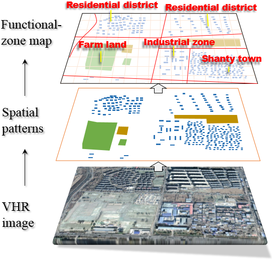
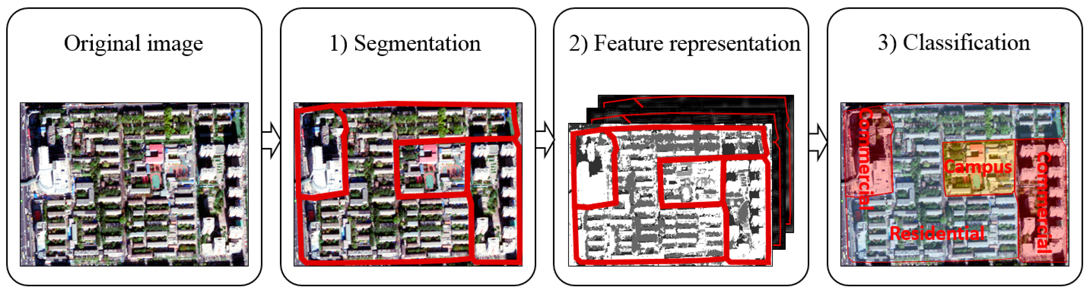
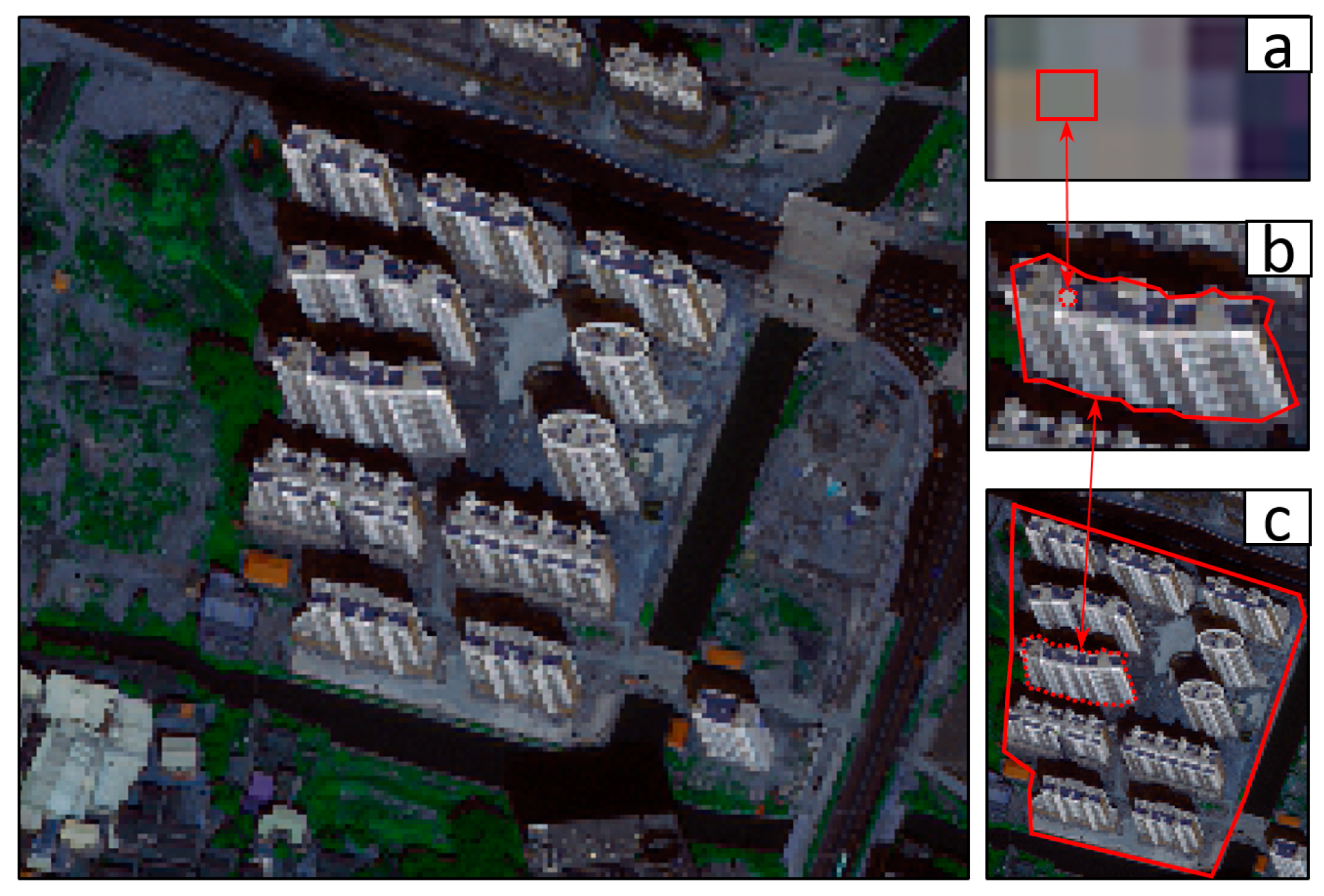
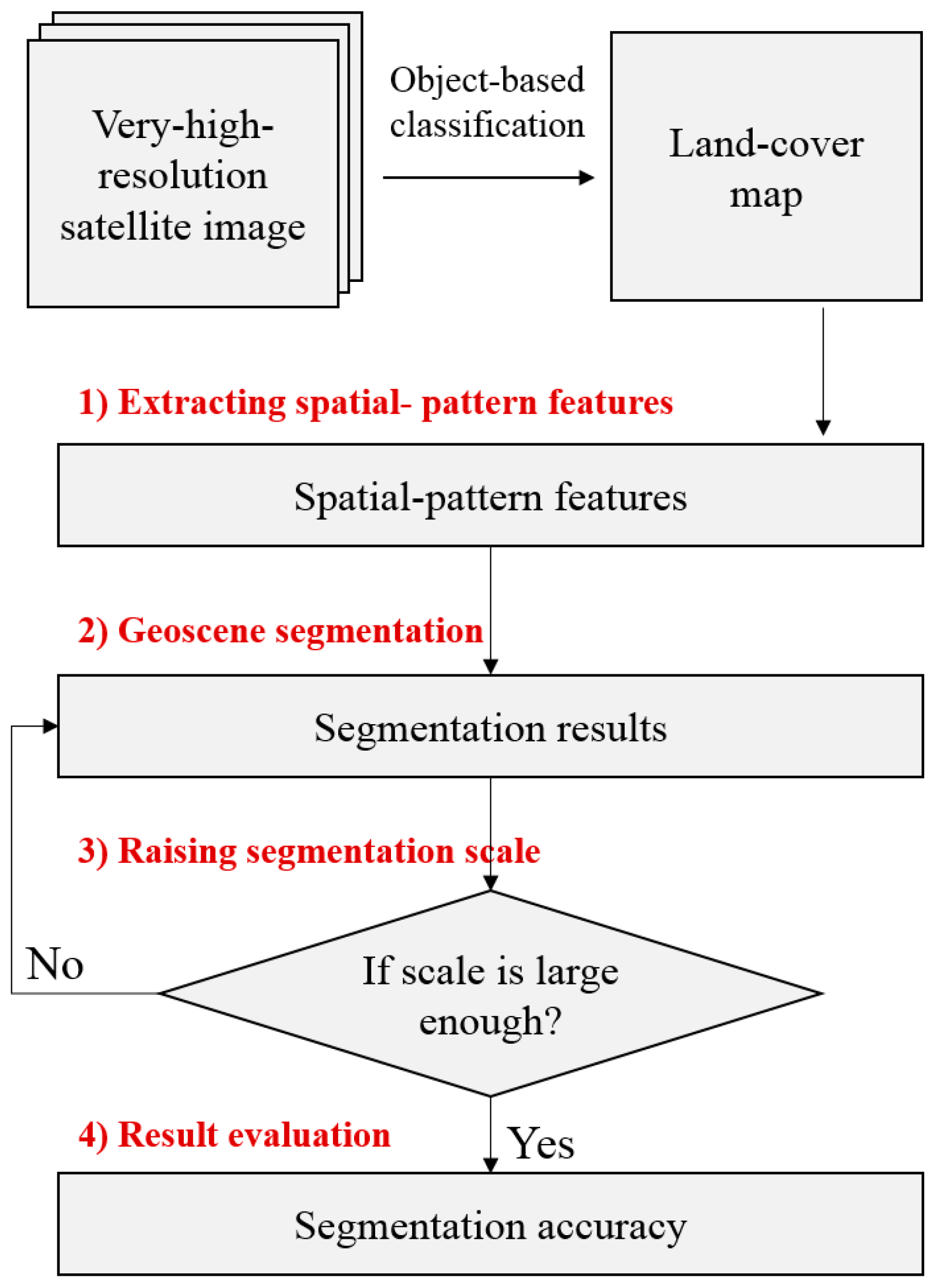
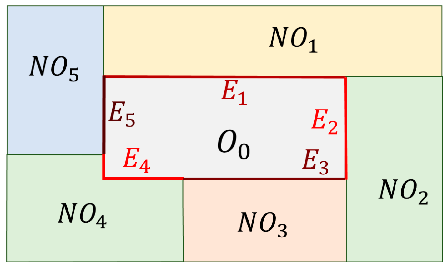
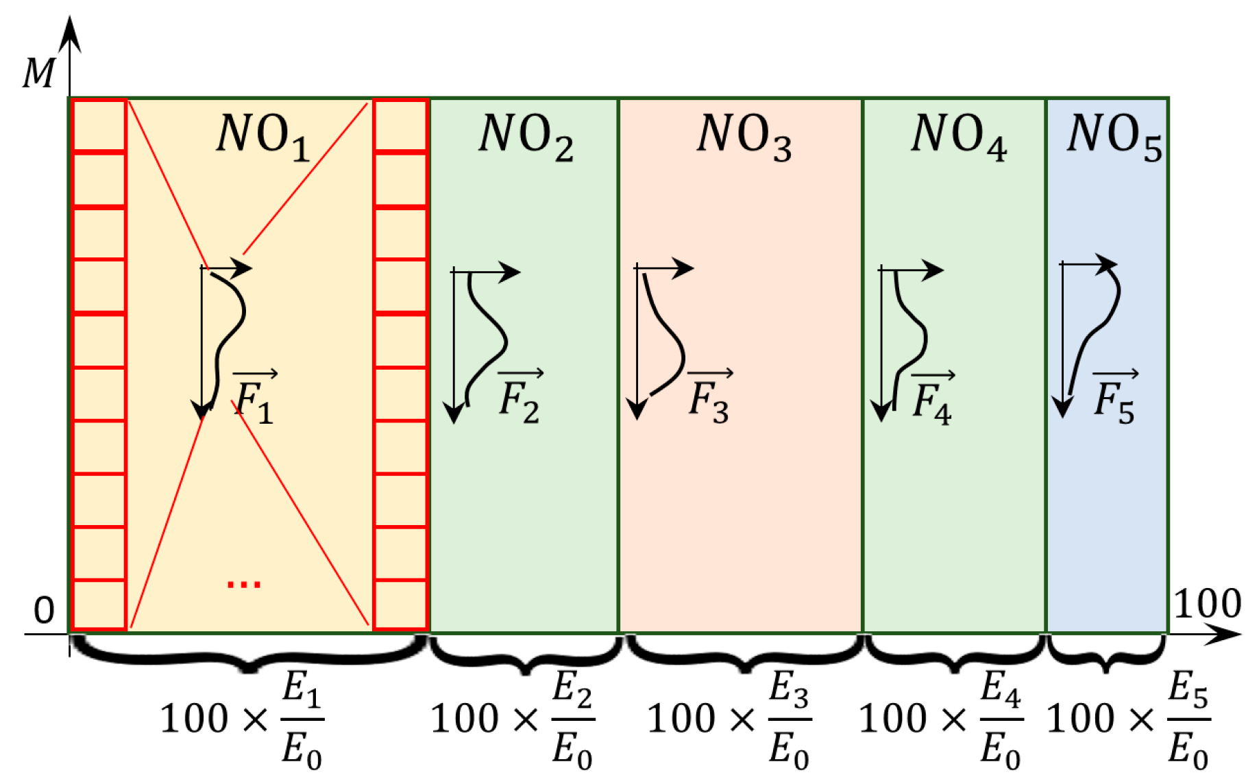
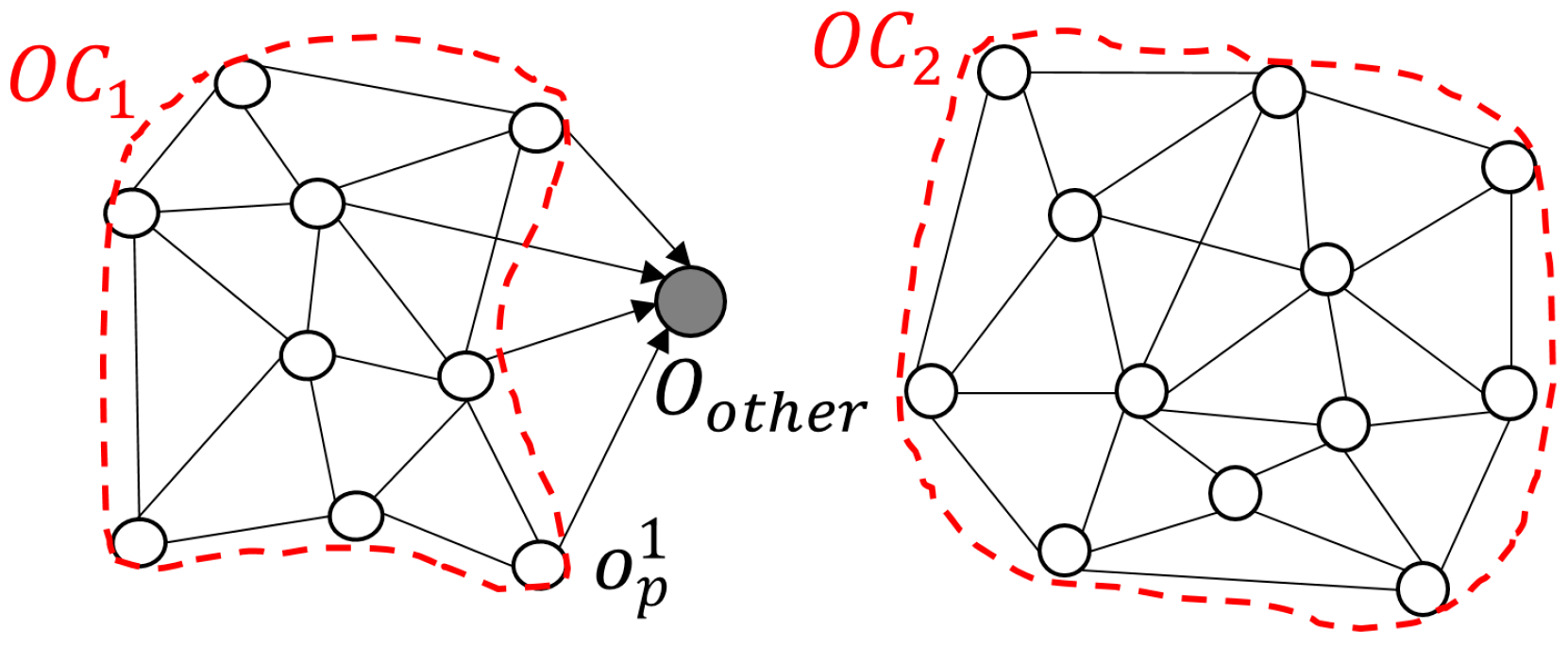
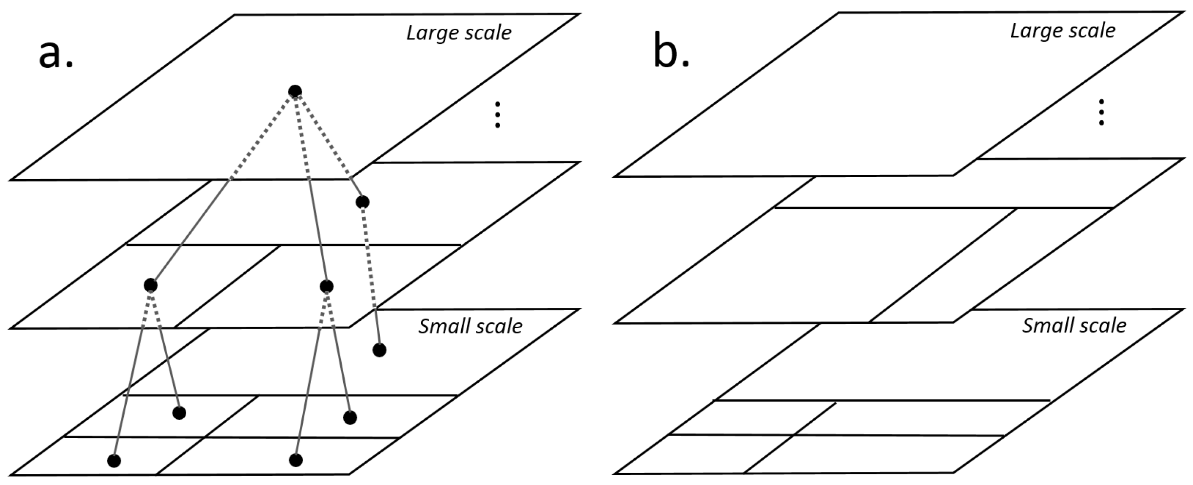
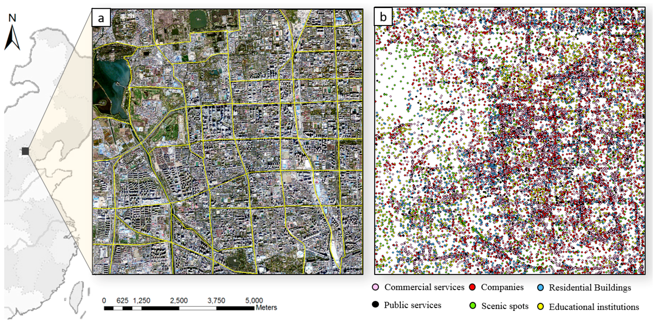
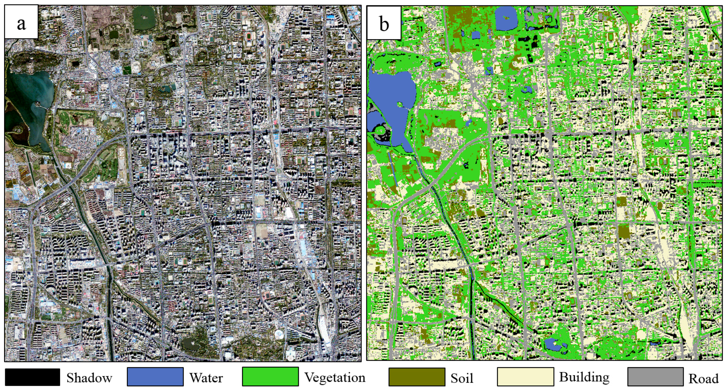
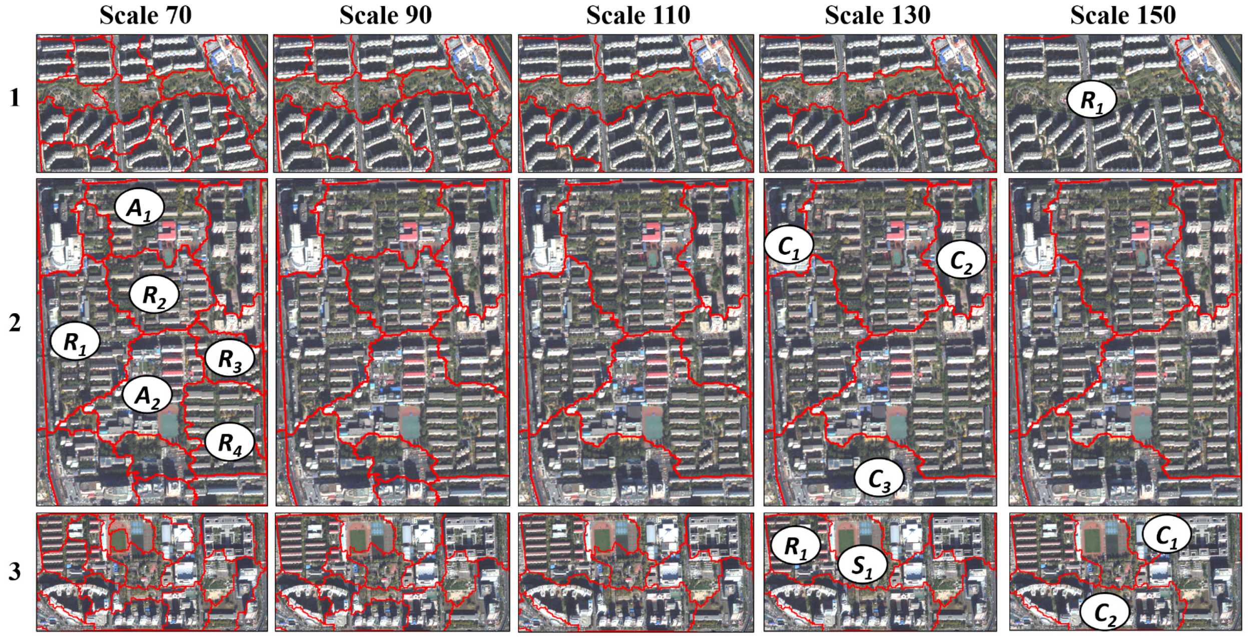
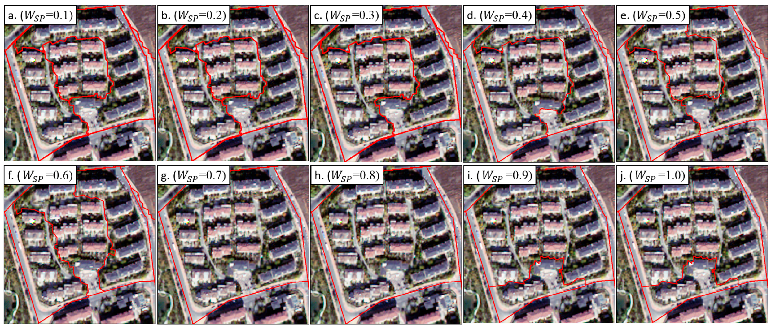
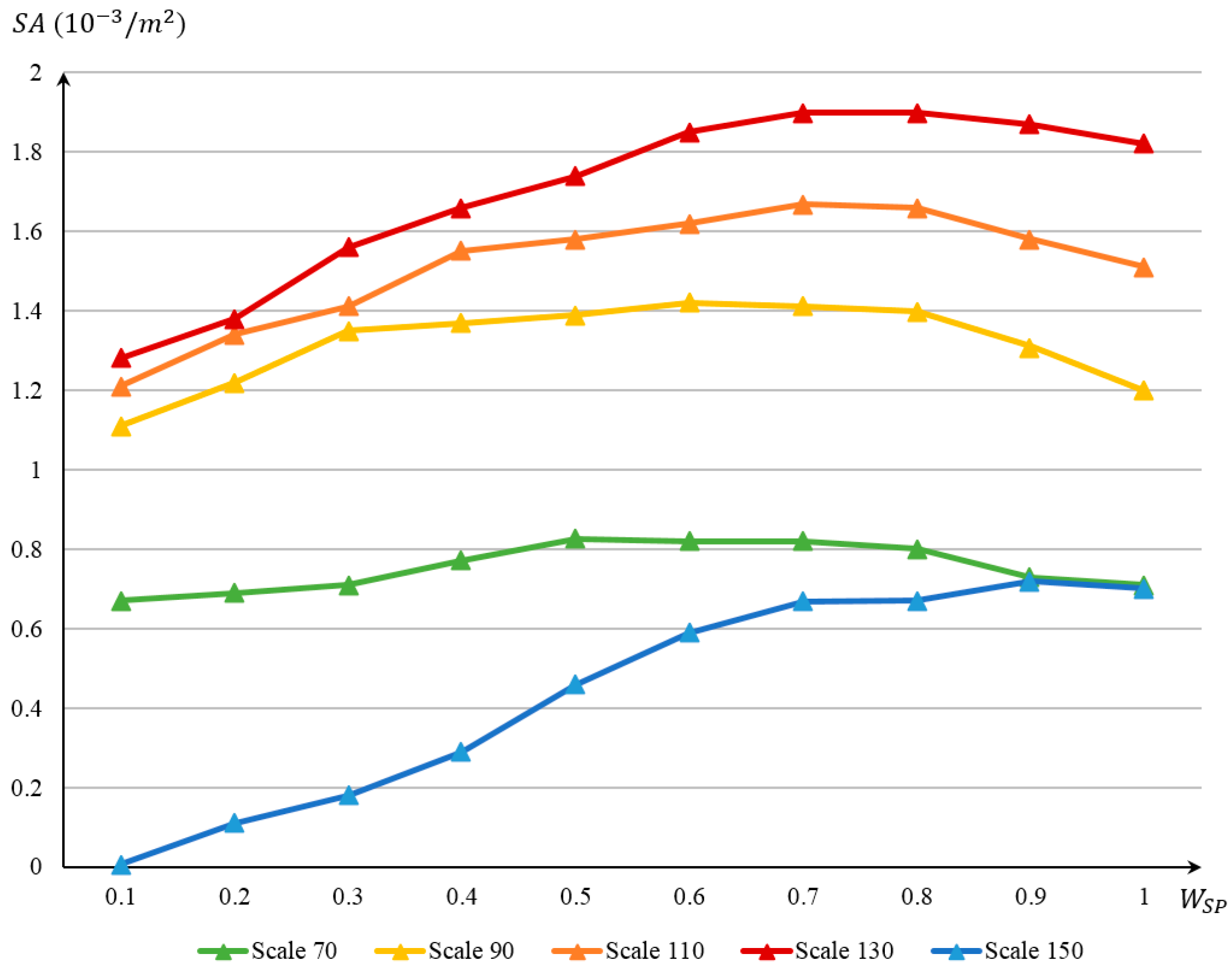
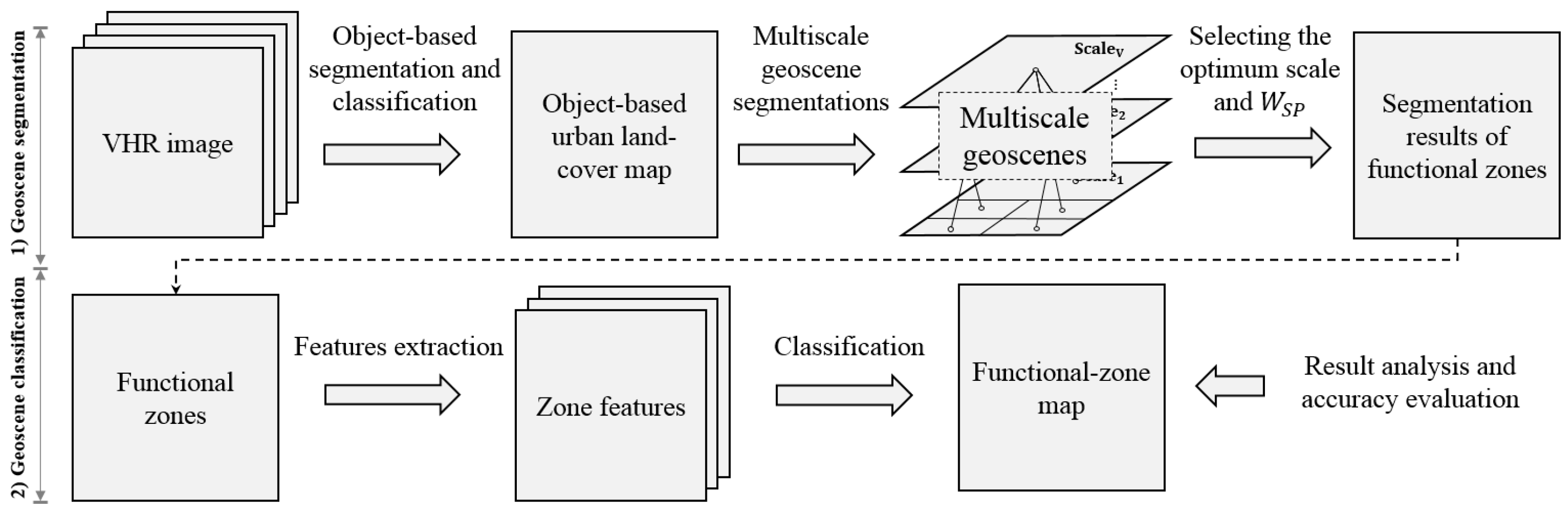
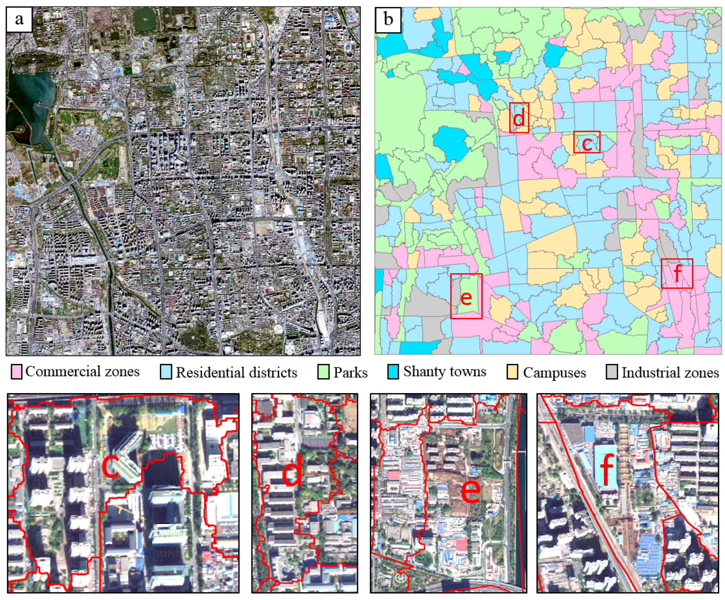
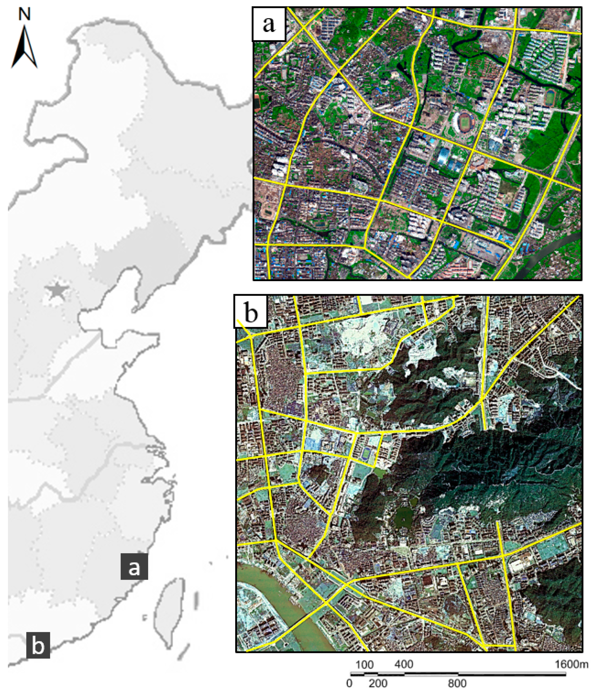
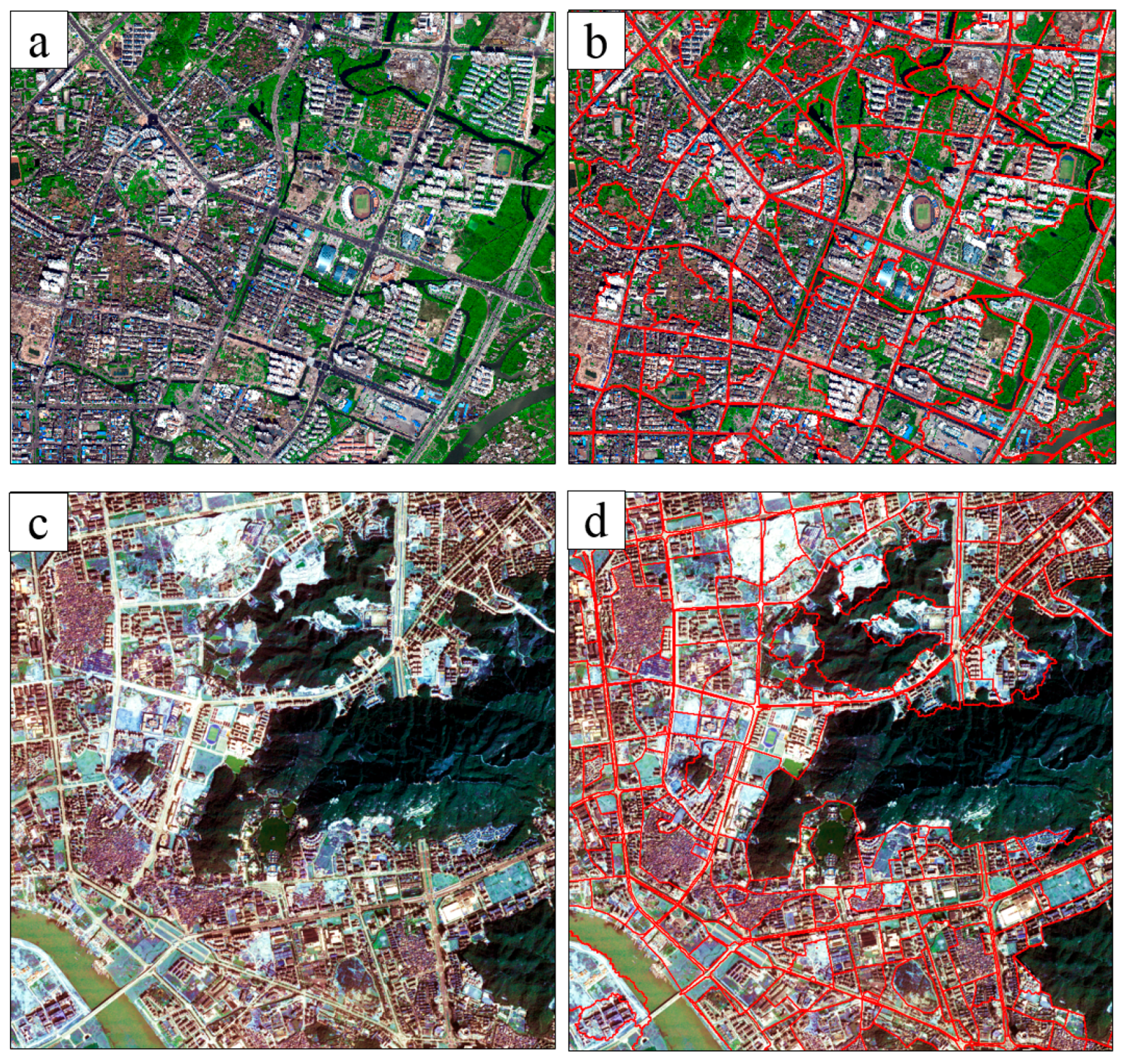
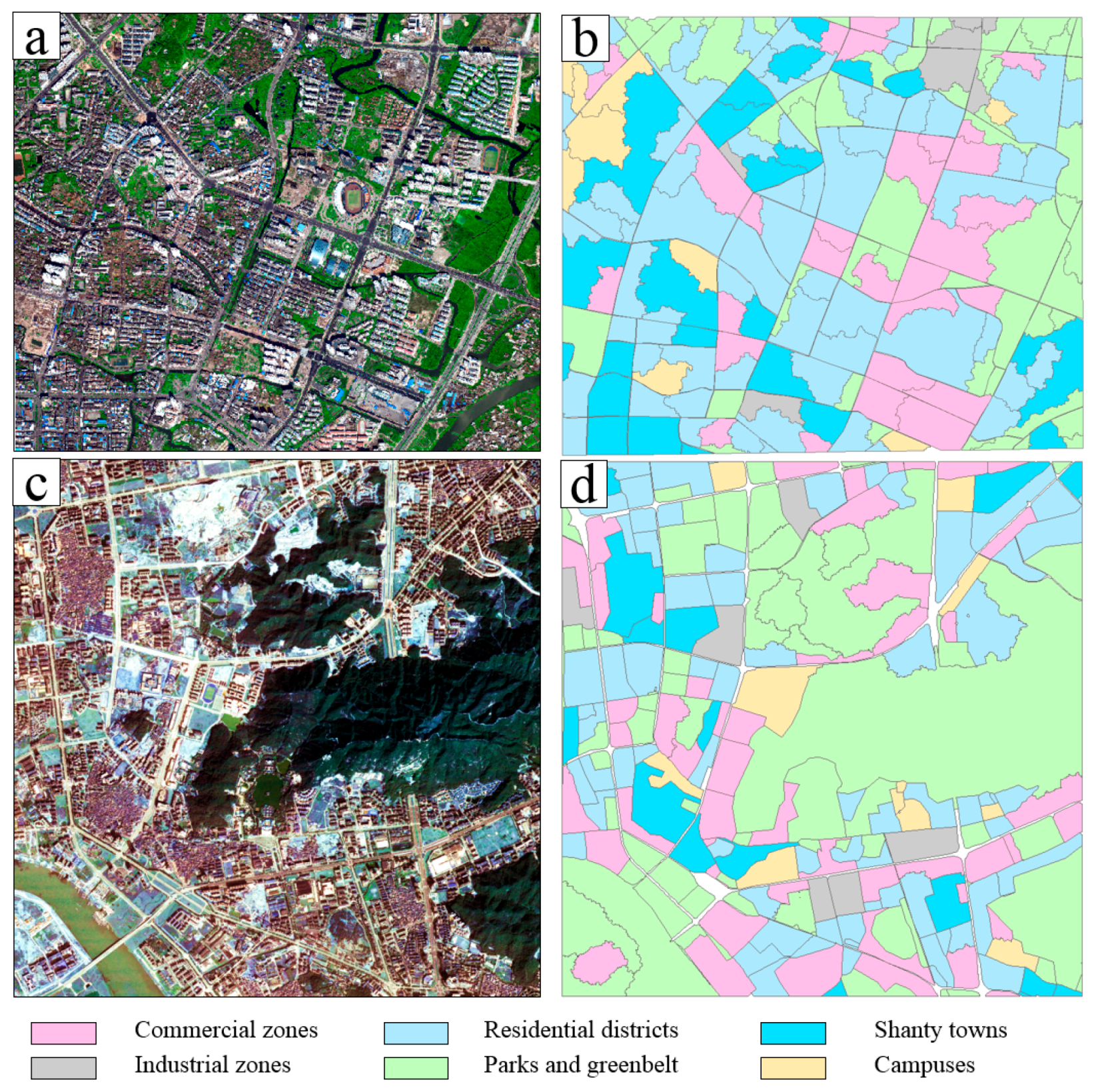
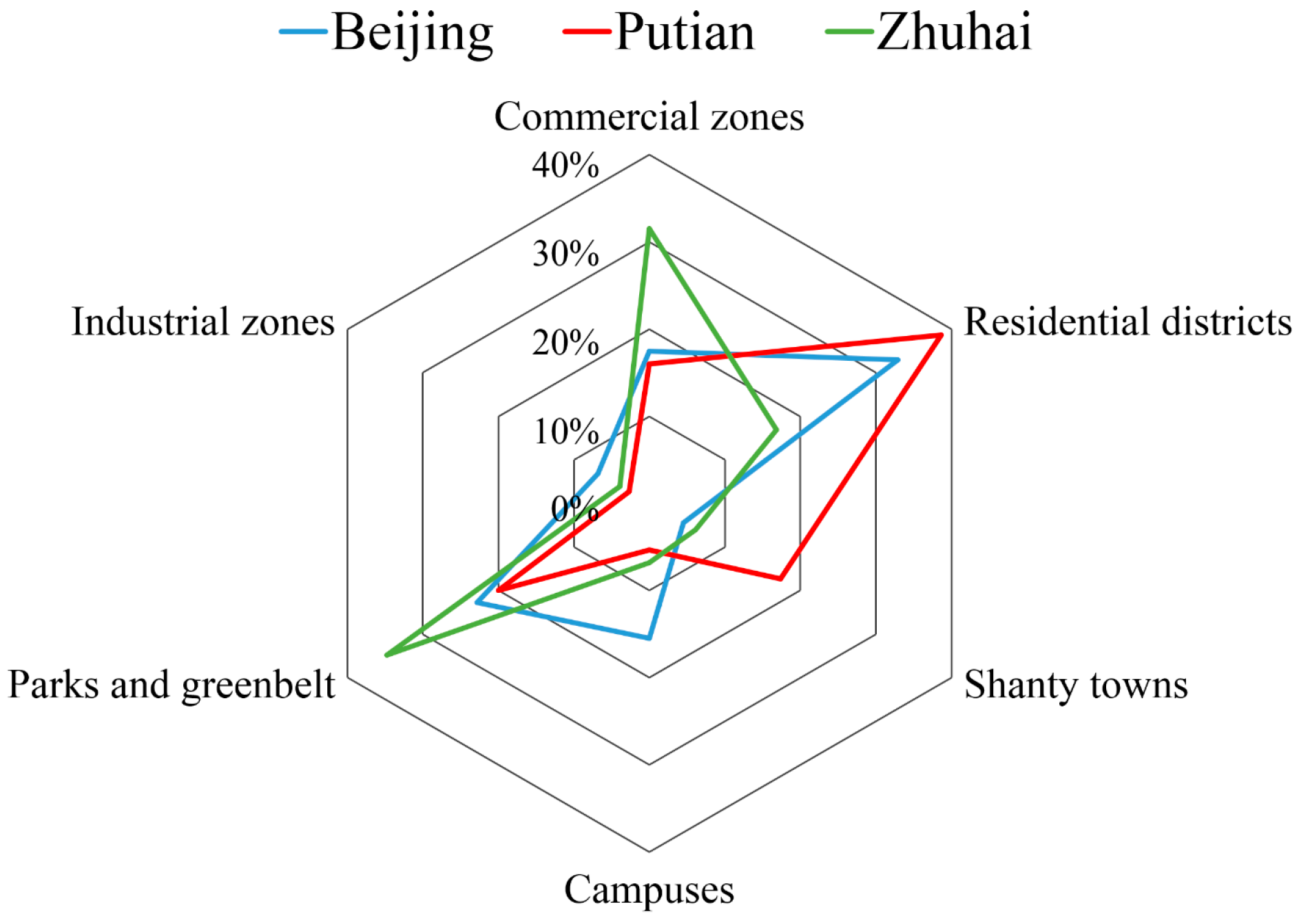
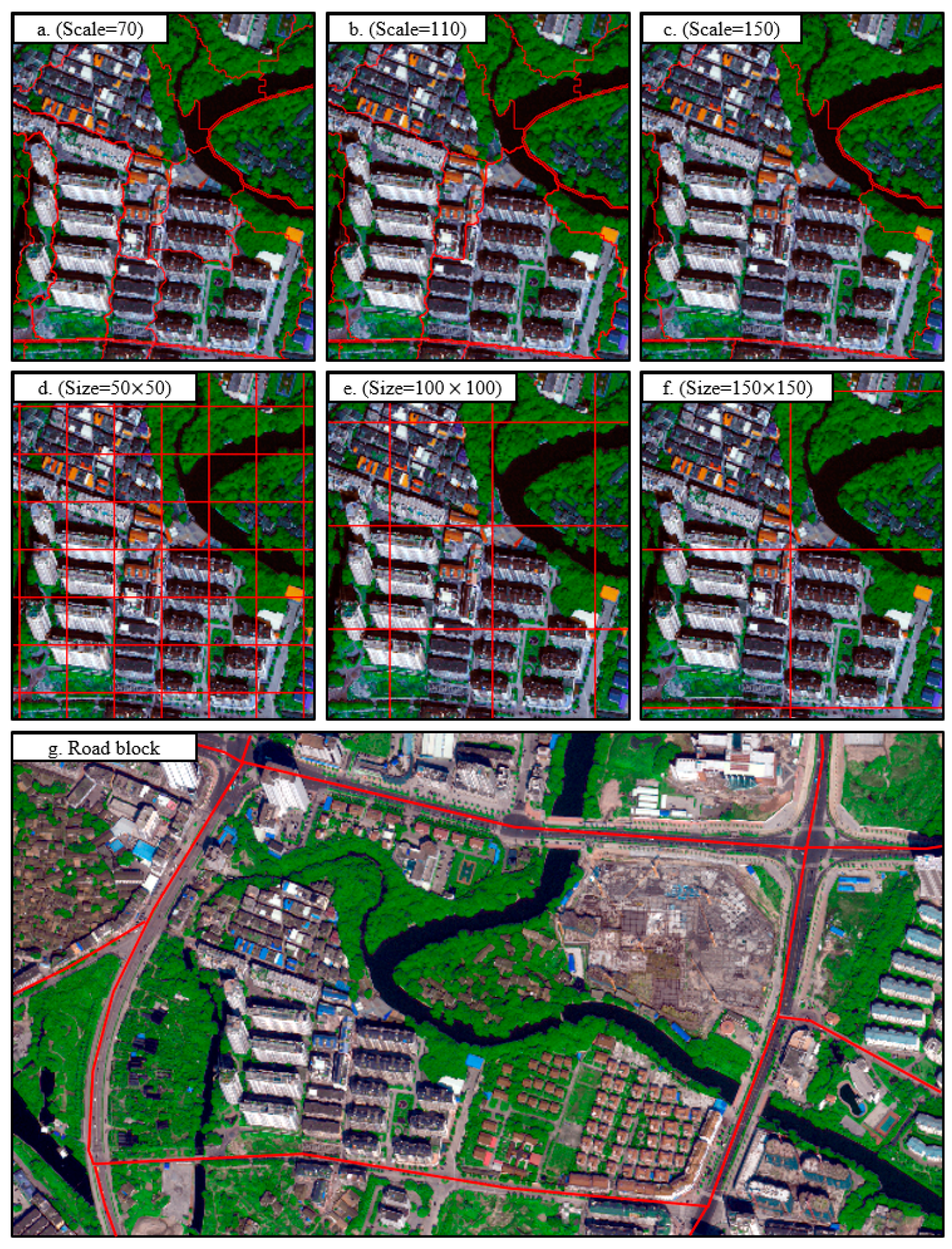
Table 1.
Relations between geographic objects and analytical units.
| Geographic Entities | Image Units | References |
|---|---|---|
| Separated trees/stones | Pixels | [29,30] |
| Woods/buildings | Objects | [31,32,33,34,35] |
| Forest ecological system/urban functional zones | Geoscenes |
Table 2.
Terminologies proposed in this study.
| Terminologies | Meaning |
|---|---|
| Functional zones | Functional zones are basic units of city planning and management which are spatially aggregations of diverse geographic objects with regular patterns, and their functional categories are semantically abstracted from objects’ land uses. |
| Geoscenes | Spatially continuous and non-overlapping regions in remote sensing images, with each one composed of diverse objects. Each geoscene comprises similar spatial patterns, in which the same-category objects have similar object and pattern characteristics. |
| Geoscene-based image analysis (GEOSBIA) | An image analysis strategy, which uses geoscenes as basic units to analyze functional zones. It mainly includes geoscene segmentation, feature extraction, and classification. This new strategy greatly differs from per-pixel and object-based image analyses in terms of features, categories, segmentations, classifications, and applications. |
| Geoscene segmentation | A strategy to partition an image into geoscenes considering both object and spatial-pattern features. |
| Geoscene segmentation scale | An important parameter for controlling geoscene segmentation results, and representing the largest tolerable heterogeneity of segmented geoscenes. |
| Spatial-pattern features | Features used for measuring spatial arrangements of objects. Spatial-pattern features are used to characterize functional zones in this study. |
Table 3.
Visual features for characterizing objects.
| Types | Names | Meanings |
|---|---|---|
| Spectral | (Mean spectrum) | Average spectrum of an object |
| (Std. dev) | Gray standard deviation in an object | |
| (Skewness) | Skewness of spectral histogram | |
| Textural | (GLDV) | The vector composed of diagonal elements of GLCM |
| (Homogeneity) | The homogeneity derived from GLCM | |
| (Dissimilarity) | The heterogeneity parameters derived from GLCM | |
| (Entropy) | Information entropy derived from GLCM | |
| (Correlation) | Correlation of pixels which is derived from GLCM | |
| Geometrical | (Area) | The number of pixels within image objects |
| (Length/width) | Length-width ratio of the object’s MBR | |
| (Main direction) | Eigenvectors of covariance matrix | |
| (Shape index) | The ratio of perimeter to four times side length |
Table 4.
Geoscene-segmentation accuracies at five scales, with referring to the number of geoscenes and representing the segmentation accuracy.
Table 4.
Geoscene-segmentation accuracies at five scales, with referring to the number of geoscenes and representing the segmentation accuracy.
| Scales | 70 | 90 | 110 | 130 | 150 |
|---|---|---|---|---|---|
| 1614 | 1067 | 830 | 703 | 218 | |
Table 5.
Confusion matrix of functional-zone classification results. Co = Commercial zones; Re = Residential districts; Sh = Shanty towns; In = Industrial zones; Pa = Parks and greenbelt; Ca = Campuses; and OA = Overall accuracy.
Table 5.
Confusion matrix of functional-zone classification results. Co = Commercial zones; Re = Residential districts; Sh = Shanty towns; In = Industrial zones; Pa = Parks and greenbelt; Ca = Campuses; and OA = Overall accuracy.
| Functions | Co | Re | Sh | In | Pa | Ca | Total | User’s Accuracy |
|---|---|---|---|---|---|---|---|---|
| Co | 109 | 11 | 0 | 2 | 10 | 0 | 132 | 82.6% |
| Re | 8 | 250 | 1 | 3 | 2 | 5 | 269 | 92.9% |
| Sh | 0 | 1 | 12 | 0 | 0 | 0 | 13 | 92.3% |
| In | 3 | 0 | 1 | 21 | 0 | 0 | 25 | 84.0% |
| Pa | 0 | 4 | 0 | 0 | 118 | 1 | 121 | 97.5% |
| Ca | 0 | 20 | 0 | 1 | 2 | 118 | 133 | 88.7% |
| Total | 120 | 286 | 14 | 27 | 132 | 124 | 703 | |
| Producer’s accuracy | 90.8% | 87.4% | 85.7% | 77.8% | 89.4% | 95.2% | OA = 89.3% |
Table 6.
Information of two QuickBird images.
| Image | Location | Data Source | Resolution | Acquisition Date | Area |
|---|---|---|---|---|---|
| Figure 18a | Putian | QuickBird | 0.61 m | 17 June 2010 | 7.5 |
| Figure 18b | Zhuhai | QuickBird | 0.61 m | 23 June 2010 | 27.9 |
Table 7.
Areas and proportions of diverse functional zones in the three study areas.
| Study Areas | Beijing | Putian | Zhuhai | |||
|---|---|---|---|---|---|---|
| Area () | Proportion | Area () | Proportion | Area () | Proportion | |
| Commercial zones | 11.7 | 17.4% | 1.2 | 16.0% | 7.8 | 31.5% |
| Residential districts | 22.1 | 32.9% | 2.9 | 38.7% | 4.7 | 16.8% |
| Shanty towns | 3.0 | 4.5% | 1.3 | 17.3% | 1.7 | 6.1% |
| Campuses | 10.4 | 15.5% | 0.4 | 5.3% | 0.9 | 6.8% |
| Parks and greenbelt | 15.3 | 22.8% | 1.5 | 20.0 % | 9.7 | 34.8% |
| Industrial zones | 4.6 | 6.9% | 0.2 | 2.7% | 3.1 | 4.0% |
| Total | 67.1 | 100% | 7.5 | 100% | 27.9 | 100% |
© 2018 by the authors. Licensee MDPI, Basel, Switzerland. This article is an open access article distributed under the terms and conditions of the Creative Commons Attribution (CC BY) license (http://creativecommons.org/licenses/by/4.0/).
Share and Cite
MDPI and ACS Style
Zhang, X.; Du, S.; Wang, Q.; Zhou, W. Multiscale Geoscene Segmentation for Extracting Urban Functional Zones from VHR Satellite Images. Remote Sens. 2018, 10, 281. https://doi.org/10.3390/rs10020281
AMA Style
Zhang X, Du S, Wang Q, Zhou W. Multiscale Geoscene Segmentation for Extracting Urban Functional Zones from VHR Satellite Images. Remote Sensing. 2018; 10(2):281. https://doi.org/10.3390/rs10020281
Chicago/Turabian StyleZhang, Xiuyuan, Shihong Du, Qiao Wang, and Weiqi Zhou. 2018. "Multiscale Geoscene Segmentation for Extracting Urban Functional Zones from VHR Satellite Images" Remote Sensing 10, no. 2: 281. https://doi.org/10.3390/rs10020281
Note that from the first issue of 2016, this journal uses article numbers instead of page numbers. See further details here.