Assessment of LiDAR and Spectral Techniques for High-Resolution Mapping of Sporadic Permafrost on the Yukon-Kuskokwim Delta, Alaska

 , ,
, ,
Abstract
:
1. Introduction
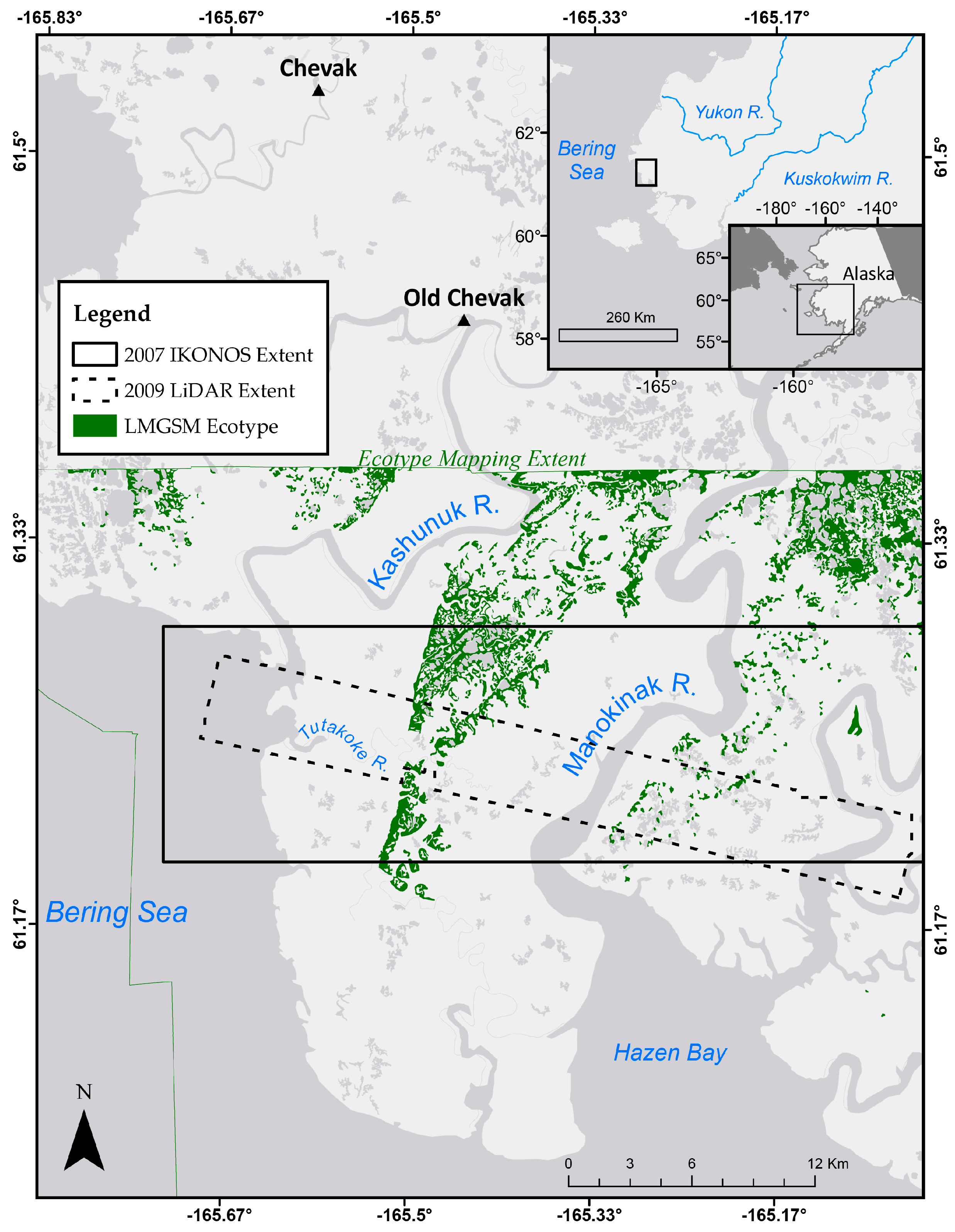
Study Area
2. Materials and Methods
2.1. Fieldwork
2.2. LiDAR Mapping
2.3. Spectral Integration
3. Results
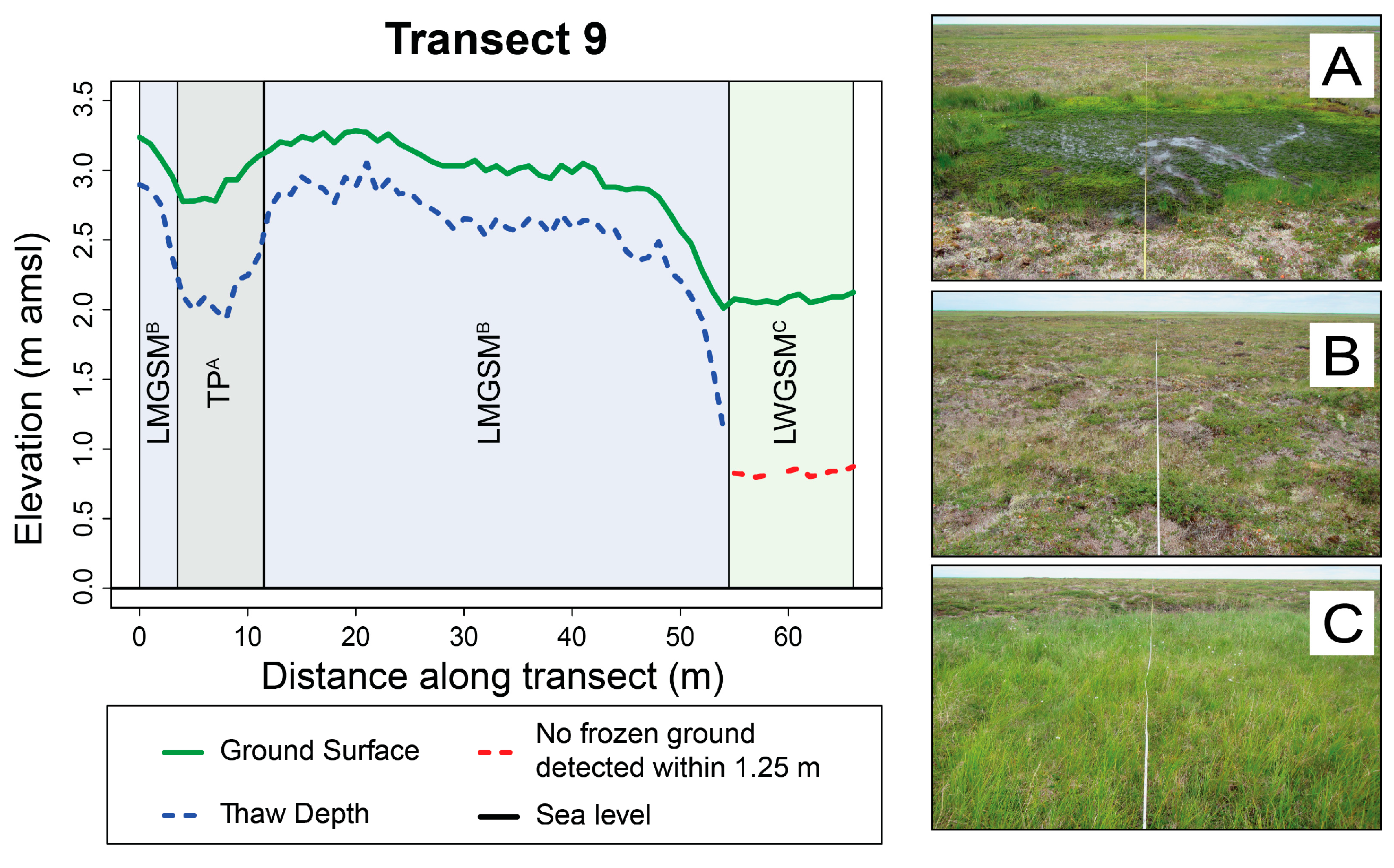
3.1. Transect Profiles
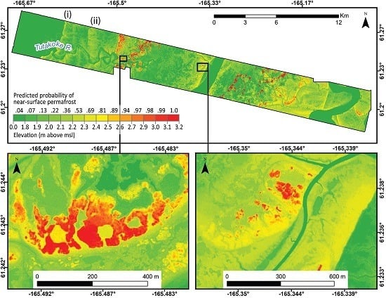
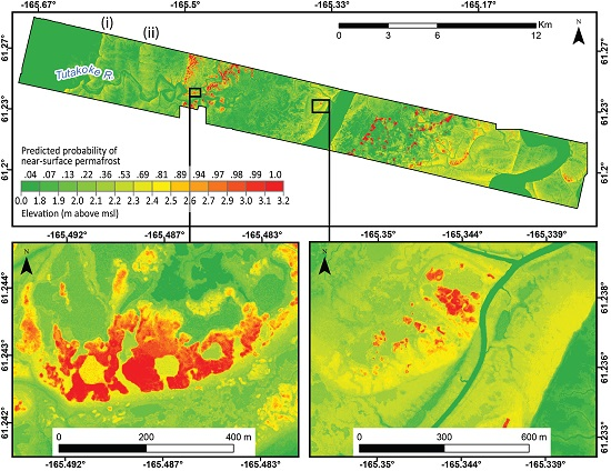
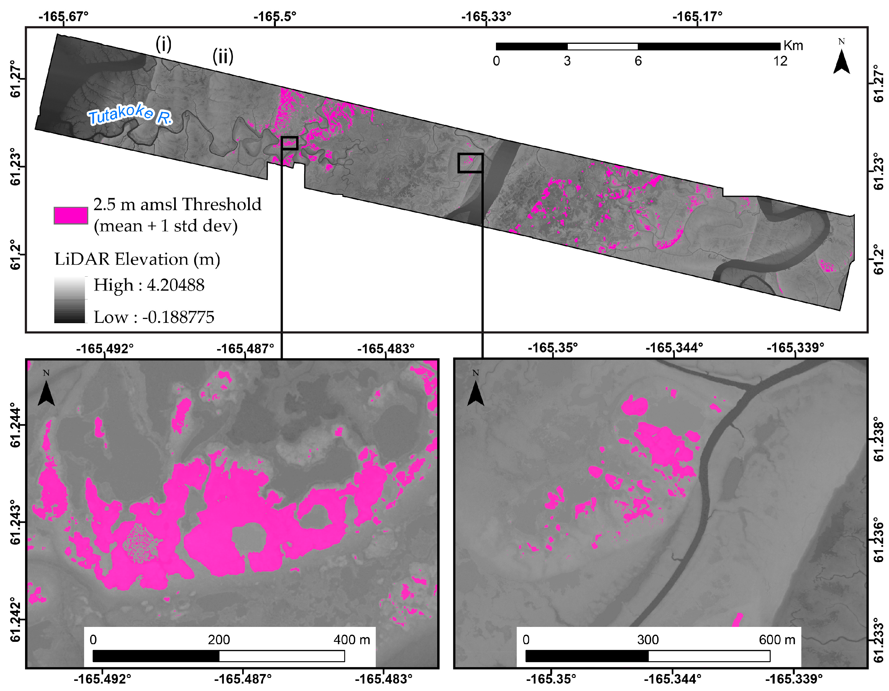
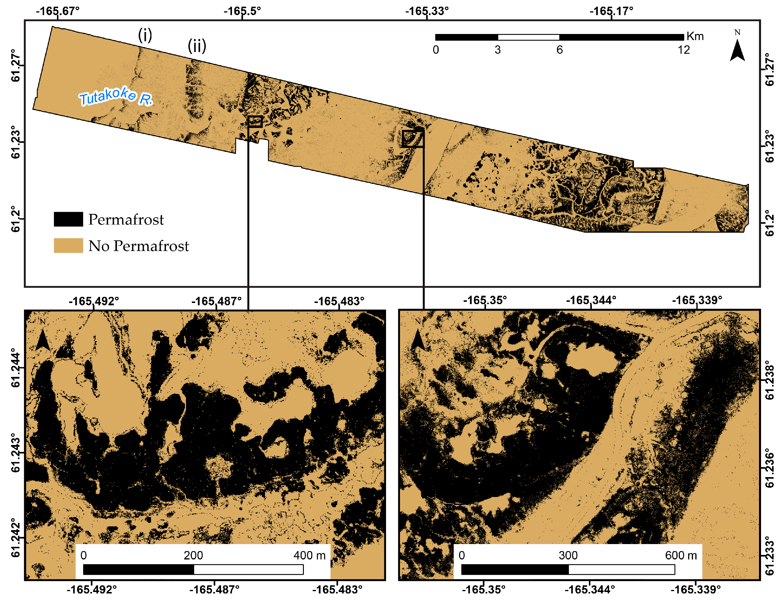
3.2. LiDAR Mapping
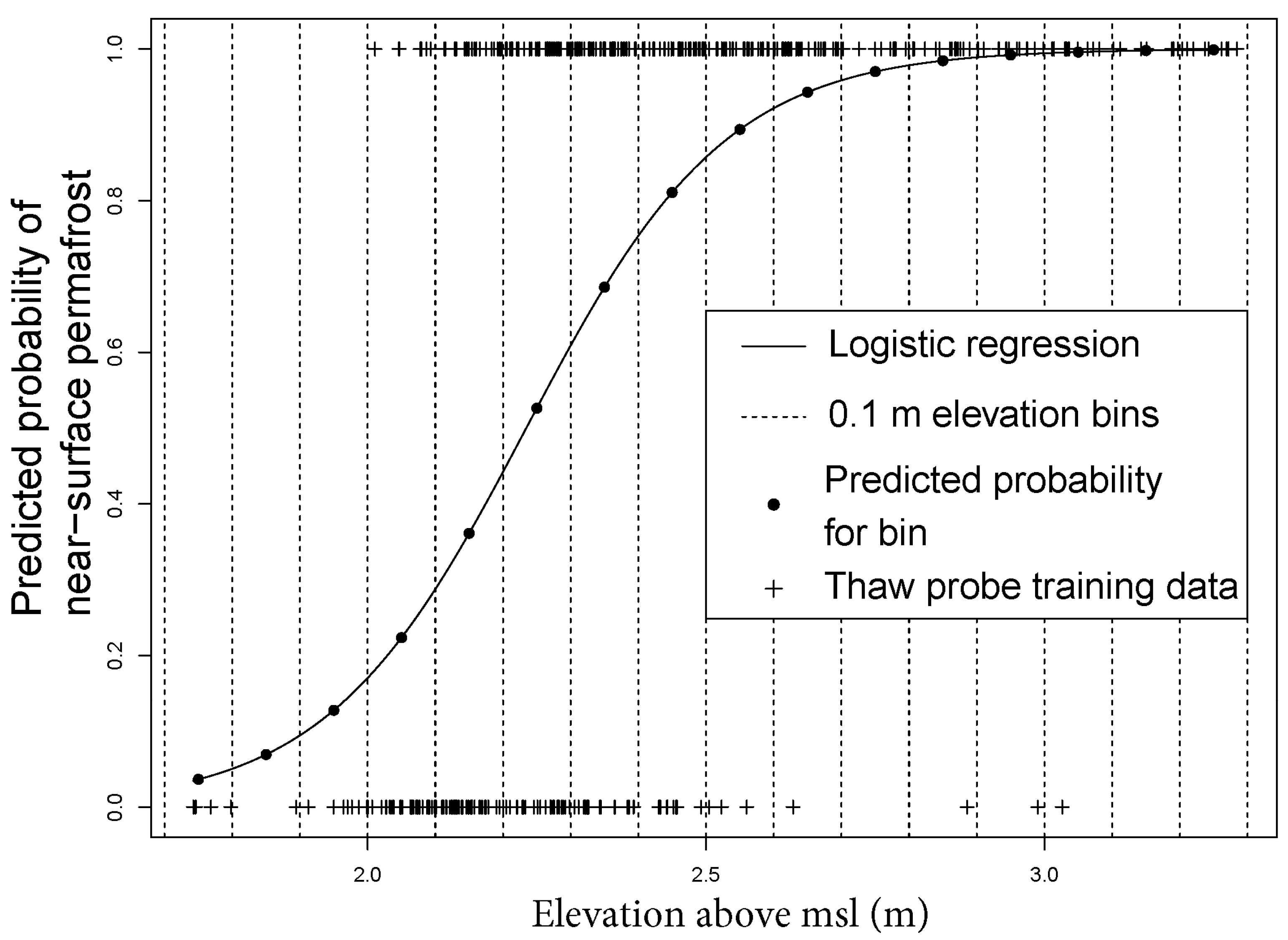
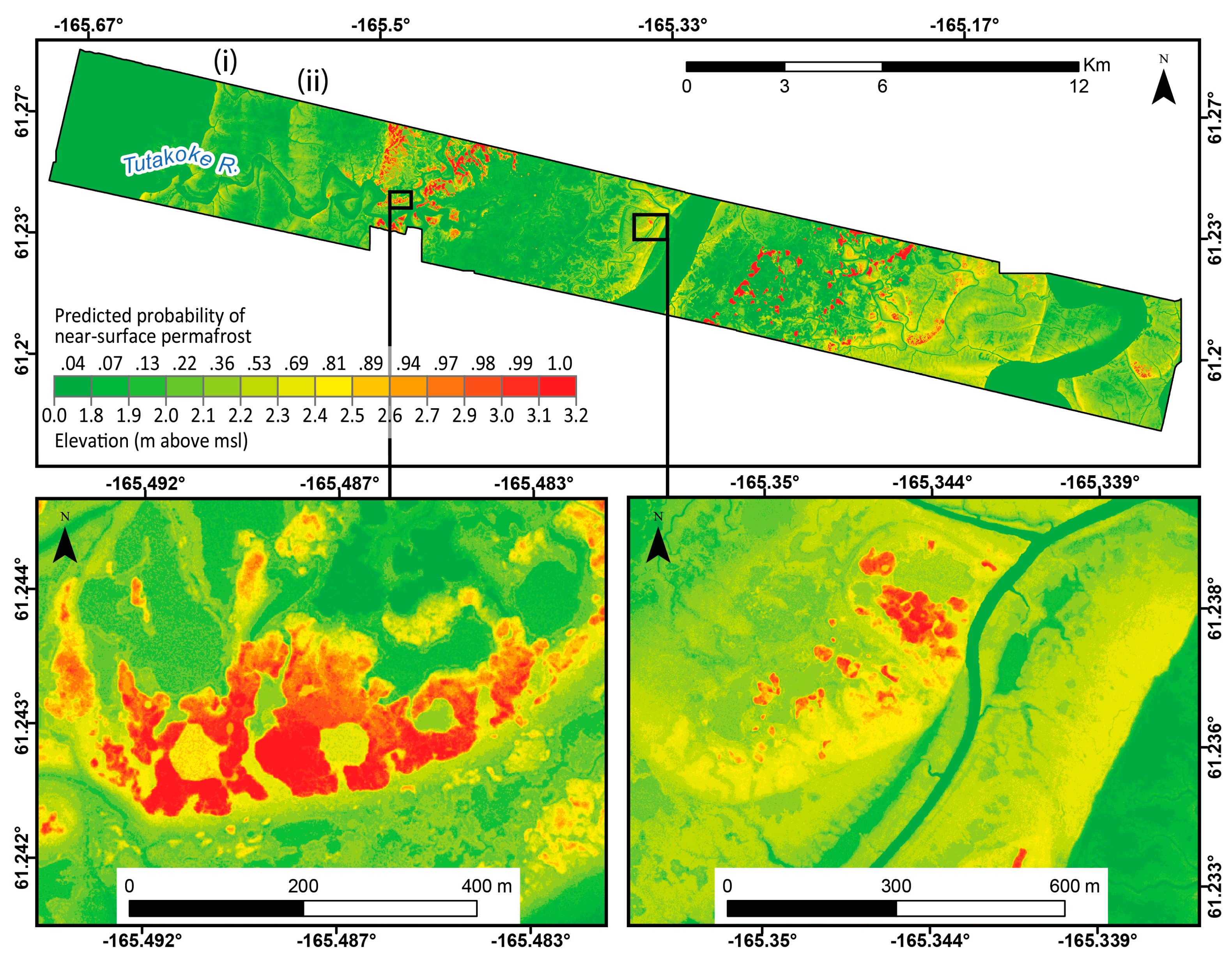
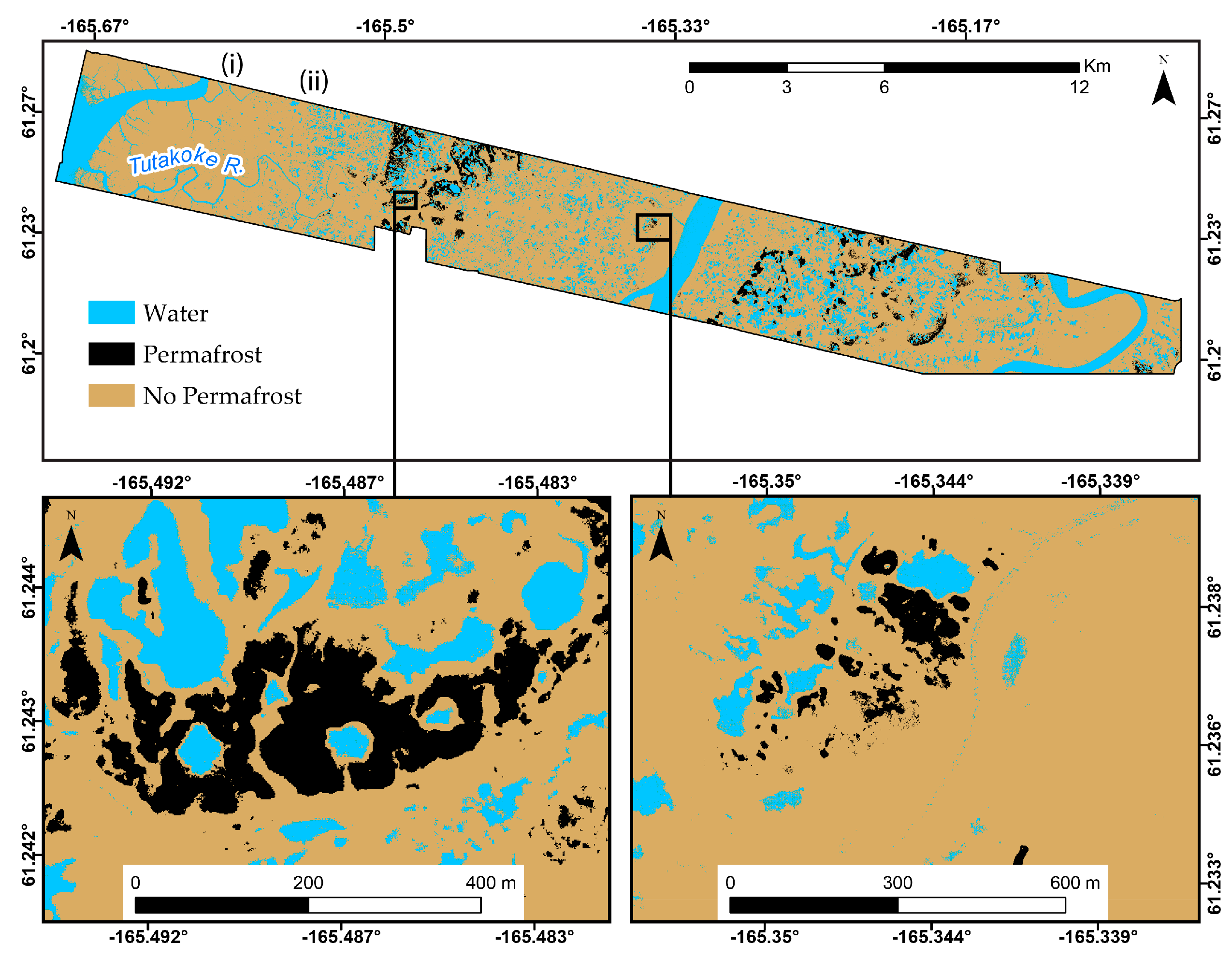
3.3. Spectral Integration
4. Discussion
4.1. Landscape Characteristics
4.2. LiDAR Mapping
4.3. Spectral Integration
4.4. Paths for Regional Scale Mapping
4.5. Broader Impacts
5. Conclusions
Acknowledgments
Author Contributions
Conflicts of Interest
References
- Brown, J.; Ferrians, O., Jr.; Heginbottom, J.; Melnikov, E. Circum-Arctic Map of Permafrost and Ground-Ice Conditions; United States Geological Survey: Reston, VA, USA, 1997. [Google Scholar]
- Jorgenson, M.T.; Yoshikawa, K.; Kanevskiy, M.; Shur, Y.; Romanovsky, V.; Marchenko, S.; Grosse, G.; Brown, J.; Jones, B. Permafrost characteristics of Alaska. In Proceedings of the Ninth International Conference on Permafrost, Fairbanks, AK, USA, 29 June–3 July 2008; pp. 121–122. [Google Scholar]
- Cuff, D.; Goudie, A. The Oxford Companion to Global Change; Oxford University Press: Oxford, UK, 2009. [Google Scholar]
- Hinzman, L.D.; Bettez, N.D.; Bolton, W.R.; Chapin, F.S.; Dyurgerov, M.B.; Fastie, C.L.; Griffith, B.; Hollister, R.D.; Hope, A.; Huntington, H.P. Evidence and implications of recent climate change in northern Alaska and other Arctic regions. Clim. Chang. 2005, 72, 251–298. [Google Scholar] [CrossRef]
- Jorgenson, M.T.; Roth, J.E. Landscape Classification and Mapping for the Yukon-Kuskokwim Delta: Final Report Prepared for: U.S. Fish and Wildlife Service; ABR, Inc.-Environmental Research & Service: Fairbanks, AK, USA, 2010; p. 24. [Google Scholar]
- Romanovsky, V.E.; Smith, S.L.; Christiansen, H.H. Permafrost thermal state in the polar northern hemisphere during the international polar year 2007–2009: A synthesis. Permafr. Periglac. Process. 2010, 21, 106–116. [Google Scholar] [CrossRef]
- Schuur, E.; McGuire, A.; Schädel, C.; Grosse, G.; Harden, J.; Hayes, D.; Hugelius, G.; Koven, C.; Kuhry, P.; Lawrence, D. Climate change and the permafrost carbon feedback. Nature 2015, 520, 171–179. [Google Scholar] [CrossRef] [PubMed]
- Liljedahl, A.K.; Boike, J.; Daanen, R.P.; Fedorov, A.N.; Frost, G.V.; Grosse, G.; Hinzman, L.D.; Iijma, Y.; Jorgenson, J.C.; Matveyeva, N. Pan-Arctic ice-wedge degradation in warming permafrost and its influence on tundra hydrology. Nat. Geosci. 2016, 9, 312–318. [Google Scholar] [CrossRef]
- Riseborough, D.; Shiklomanov, N.; Etzelmüller, B.; Gruber, S.; Marchenko, S. Recent advances in permafrost modelling. Permafr. Periglac. Process. 2008, 19, 137–156. [Google Scholar] [CrossRef]
- Pastick, N.J.; Jorgenson, M.T.; Wylie, B.K.; Nield, S.J.; Johnson, K.D.; Finley, A.O. Distribution of near-surface permafrost in Alaska: Estimates of present and future conditions. Remote Sens. Environ. 2015, 168, 301–315. [Google Scholar] [CrossRef]
- Jafarov, E.E.; Marchenko, S.S.; Romanovsky, V. Numerical modeling of permafrost dynamics in Alaska using a high spatial resolution dataset. Cryosphere 2012, 6, 613–624. [Google Scholar] [CrossRef] [Green Version]
- Zhang, Y.; Chen, W.; Riseborough, D.W. Disequilibrium response of permafrost thaw to climate warming in Canada over 1850–2100. Geophys. Res. Lett. 2008, 35. [Google Scholar] [CrossRef]
- Slater, A.G.; Lawrence, D.M. Diagnosing present and future permafrost from climate models. J. Clim. 2013, 26, 5608–5623. [Google Scholar] [CrossRef]
- Heginbottom, J.A. Permafrost mapping: A review. Prog. Phys. Geogr. 2002, 26, 623–642. [Google Scholar] [CrossRef]
- Jorgenson, M.T.; Grosse, G. Remote sensing of landscape change in permafrost regions. Permafr. Periglac. Process. 2016, 27, 324–338. [Google Scholar] [CrossRef]
- Gogineni, P.; Romanovsky, V.; Cherry, J.; Duguay, C.; Goetz, S.; Jorgenson, M.; Moghaddami, M. Opportunities to Use Remote Sensing in Understanding Permafrost and Related Ecological Characteristics: Report of a Workshop; National Academies Press: Washington, DC, USA, 2014; p. 97. [Google Scholar]
- Westermann, S.; Østby, T.; Gisnås, K.; Schuler, T.; Etzelmüller, B. A ground temperature map of the North Atlantic permafrost region based on remote sensing and reanalysis data. Cryosphere 2015, 9, 1303–1319. [Google Scholar] [CrossRef]
- Jones, B.M.; Grosse, G.; Arp, C.D.; Miller, E.; Liu, L.; Hayes, D.J.; Larsen, C.F. Recent Arctic tundra fire initiates widespread thermokarst development. Sci. Rep. 2015, 5, 15865. [Google Scholar] [CrossRef] [PubMed] [Green Version]
- Jones, B.M.; Stoker, J.M.; Gibbs, A.E.; Grosse, G.; Romanovsky, V.E.; Douglas, T.A.; Kinsman, N.E.; Richmond, B.M. Quantifying landscape change in an Arctic coastal lowland using repeat airborne LiDAR. Environ. Res. Lett. 2013, 8, 045025. [Google Scholar] [CrossRef]
- Paine, J.G.; Andrews, J.R.; Saylam, K.; Tremblay, T.A.; Averett, A.R.; Caudle, T.L.; Meyer, T.; Young, M.H. Airborne LiDAR on the Alaskan North Slope: Wetlands mapping, lake volumes, and permafrost features. Lead. Edge 2013, 32, 798–805. [Google Scholar] [CrossRef]
- Thorsteinson, L.K.; Becker, P.R.; Hale, D.A. The Yukon Delta: A Synthesis of Information; OCS Study, MMs 89-0081; National Oceanic Atmospheric Administration: Anchorage, AK, USA, 1989; p. 89.
- Klein, D.R. Waterfowl in the economy of the eskimos on the Yukon-Kuskokwim Delta, Alaska. Arctic 1966, 19, 319–336. [Google Scholar] [CrossRef]
- Fienup-Riordan, A.; Rearden, A. Ellavut/Our Yup’ik World and Weather: Continuity and Change on the Bering Sea Coast; University of Washington Press: Seattle, WA, USA, 2013. [Google Scholar]
- Jorgenson, T.; Ely, C. Topography and flooding of coastal ecosystems on the Yukon-Kuskokwim Delta, Alaska: Implications for sea-level rise. J. Coast. Res. 2001, 17, 124–136. [Google Scholar]
- Terenzi, J.; Jorgenson, M.T.; Ely, C.R.; Giguère, N. Storm-surge flooding on the Yukon-Kuskokwim Delta, Alaska. Arctic 2014, 67, 360–374. [Google Scholar] [CrossRef]
- Péwé, R.; Brown, T. Distribution of permafrost in North America and its relationship to the environment: A review, 1963–1973. In Permafrost: North American Contribution [to The] Second International Conference; National Academies: Washington, DC, USA, 1973; p. 71. [Google Scholar]
- NOAA/NCDC. Daily Temperature Record for Bethel Airport, AK US 1923–2016; ghcnd:Usw00026615; National Oceanic and Atmospheric Administration (NOAA): Silver Spring, MD, USA, 2017.
- Shur, Y.; Jorgenson, M. Patterns of permafrost formation and degradation in relation to climate and ecosystems. Permafr. Periglac. Process. 2007, 18, 7–19. [Google Scholar] [CrossRef]
- Jorgenson, M.T. Hierarchical organization of ecosystems at multiple spatial scales on the Yukon-Kuskokwim Delta, Alaska, USA. Arct. Antarct. Alp. Res. 2000, 32, 221–239. [Google Scholar] [CrossRef]
- Tyrtikov, A.P. Perennially frozen ground and vegetation. In Principles of Geocryology (Permafrost Studies), Part I, General Geocryology, Chapter XII; Academy of Sciences of the U.S.S.R.: Moscow, Russia, 1964. [Google Scholar]
- Dunnett, C.W. Pairwise multiple comparisons in the homogeneous variance, unequal sample size case. J. Am. Stat. Assoc. 1980, 75, 789–795. [Google Scholar] [CrossRef]
- Airborne Imaging. Final LiDAR processing & vertical accuracy report: Prepared for the U.S. Fish and Wildlife Service. In LiDAR Imagery & DEM Model for Yukon Delta National Wildlife Refuge—Near Angyaravak Bay, Alaska; Airborne Imaging: Calgary, AB, Canada, 2011; p. 28. [Google Scholar]
- Lillesand, T.; Kiefer, R.W.; Chipman, J. Remote Sensing and Image Interpretation; John Wiley & Sons: Hoboken, NJ, USA, 2014. [Google Scholar]
- ESRI. Arcgis Desktop: Release 10.4; Enivronmental Systems Research Institute: Redlands, CA, USA, 2015. [Google Scholar]
- Breiman, L. Random forests. Mach. Learn. 2001, 45, 5–32. [Google Scholar] [CrossRef]
- Panda, S.K.; Prakash, A.; Solie, D.N.; Romanovsky, V.E.; Jorgenson, M.T. Remote sensing and field-based mapping of permafrost distribution along the Alaska highway corridor, Interior Alaska. Permafr. Periglac. Process. 2010, 21, 271–281. [Google Scholar] [CrossRef]
- Blok, D.; Heijmans, M.; Schaepman-Strub, G.; van Ruijven, J.; Parmentier, F.; Maximov, T.; Berendse, F. The cooling capacity of mosses: Controls on water and energy fluxes in a Siberian tundra site. Ecosystems 2011, 14, 1055–1065. [Google Scholar] [CrossRef] [Green Version]
- Kokelj, S.; Jorgenson, M. Advances in thermokarst research. Permafr. Periglac. Process. 2013, 24, 108–119. [Google Scholar] [CrossRef]
- Duk-Rodkin, A.; Barendregt, R.; White, J.; Singhroy, V. Geologic evolution of the Yukon River: Implications for placer gold. Quat. Int. 2001, 82, 5–31. [Google Scholar] [CrossRef]
- Dupré, W.R. Yukon Delta Coastal Processes Study; Department of Geology, University of Houston: Houston, TX, USA, 1980. [Google Scholar]
- Douglas, T.A.; Jorgenson, M.T.; Brown, D.R.; Campbell, S.W.; Hiemstra, C.A.; Saari, S.P.; Bjella, K.; Liljedahl, A.K. Degrading permafrost mapped with electrical resistivity tomography, airborne imagery and LiDAR, and seasonal thaw measurements. Geophysics 2015, 81, WA71–WA85. [Google Scholar] [CrossRef]
- USGS-3DEP. U.S. Geological Survey Broad Agency Announcement for 3D Elevation Program (3DEP) g15ps00558; United States Geological Survey: Reston, VA, USA, 2015; pp. 1–20.
- Murphy, K. Agency Priorities for 3DEP Lidar Collection—Yukon-Kuskokwim Delta. Western Alaska Landscape Conservation Cooperative (WALCC). 2016. Available online: https://eros.usgs.gov/doi-remote-sensing-activities/2016/lidar-collection-outer-coastal-regions-yukon-and-kuskokwim-river-deltas (accessed on 5 February 2018).
- Polar Geospatial Center. ArcticDEM; Center, P.G., Ed.; University of Minnesota: Minneapolis, MN, USA, 2017. [Google Scholar]
- Bhatt, U.S.; Walker, D.A.; Walsh, J.E.; Carmack, E.C.; Frey, K.E.; Meier, W.N.; Moore, S.E.; Parmentier, F.-J.W.; Post, E.; Romanovsky, V.E.; et al. Implications of Arctic sea ice decline for the earth system. Annu. Rev. Environ. Res. 2014, 39, 57–89. [Google Scholar] [CrossRef]
- Macander, M.; Swingley, C.; Parr, C.; Sturm, M.; Selkowitz, D.; Larsen, C. Snow Depth and Snow Persistence Patterns in the Arctic from Analysis of the Entire Landsat Archive; AGU Fall Meeting Abstracts: San Francisco, CA, USA, 2016. [Google Scholar]
- Marks, J.; Tibbitts, T.; Gill, R.; McCaffery, B. Bristle-thighed curlew (Numenius tahitiensis). Birds N. Am. 2002, 705, 1–36. [Google Scholar] [CrossRef]


| Ecotype | Acronym | n | Percent Frozen Ground |
|---|---|---|---|
| Water | W | 7 | 0.0% |
| Lowland Wet Graminoid Sedge Meadow | LWGSM | 35 | 5.7% |
| Lowland Wet Sedge-Shrub Meadow | LWSSM | 60 | 10.0% |
| Riverine Moist Graminoid Shrub Meadow | RMGSM | 23 | 21.7% |
| Lowland Wet Sedge Meadow | LWSM | 40 | 40.0% |
| Thermokarst Pit | TP | 21 | 85.7% |
| Lowland Moist Graminoid Shrub Meadow | LMGSM | 292 | 94.9% |
| Wrack Line | WL | 15 | 100.0% |
| Total | 493 | 68.9% |
| Field Data | |||||
|---|---|---|---|---|---|
| Absent | Present | Row Total | User’s Accuracy | ||
| Mapped | Absent | 259 | 14 | 273 | 94.9% |
| Present | 3 | 57 | 60 | 95.0% | |
| Column Total | 262 | 71 | 333 | - | |
| Producer’s accuracy | 98.9% | 80.3% | - | - | |
| Overall Accuracy | - | - | - | 94.9% | |
| Field Data | |||||
|---|---|---|---|---|---|
| Absent | Present | Row Total | User’s Accuracy | ||
| Mapped | Absent | 259 | 15 | 274 | 94.5% |
| Present | 3 | 56 | 59 | 94.9% | |
| Column Total | 262 | 71 | 333 | - | |
| Producer’s accuracy | 98.9% | 78.9% | - | - | |
| Overall Accuracy | - | - | - | 94.6% | |
| Field Data | |||||
|---|---|---|---|---|---|
| Absent | Present | Row Total | User’s Accuracy | ||
| Mapped | Absent | 229 | 2 | 274 | 99.1% |
| Present | 33 | 69 | 59 | 67.6% | |
| Column Total | 262 | 71 | 333 | - | |
| Producer’s accuracy | 87.4% | 97.2% | - | - | |
| Overall Accuracy | - | - | - | 89.5% | |
| Field Data | |||||
|---|---|---|---|---|---|
| Absent | Present | Row Total | User’s Accuracy | ||
| Mapped | Absent | 258 | 15 | 274 | 94.5% |
| Present | 4 | 56 | 59 | 93.3% | |
| Column Total | 262 | 71 | 333 | - | |
| Producer’s accuracy | 98.5% | 79.8% | - | - | |
| Overall Accuracy | - | - | - | 94.3% | |
© 2018 by the authors. Licensee MDPI, Basel, Switzerland. This article is an open access article distributed under the terms and conditions of the Creative Commons Attribution (CC BY) license (http://creativecommons.org/licenses/by/4.0/).
Share and Cite
Whitley, M.A.; Frost, G.V.; Jorgenson, M.T.; Macander, M.J.; Maio, C.V.; Winder, S.G. Assessment of LiDAR and Spectral Techniques for High-Resolution Mapping of Sporadic Permafrost on the Yukon-Kuskokwim Delta, Alaska. Remote Sens. 2018, 10, 258. https://doi.org/10.3390/rs10020258
Whitley MA, Frost GV, Jorgenson MT, Macander MJ, Maio CV, Winder SG. Assessment of LiDAR and Spectral Techniques for High-Resolution Mapping of Sporadic Permafrost on the Yukon-Kuskokwim Delta, Alaska. Remote Sensing. 2018; 10(2):258. https://doi.org/10.3390/rs10020258
Chicago/Turabian StyleWhitley, Matthew A., Gerald V. Frost, M. Torre Jorgenson, Matthew J. Macander, Chris V. Maio, and Samantha G. Winder. 2018. "Assessment of LiDAR and Spectral Techniques for High-Resolution Mapping of Sporadic Permafrost on the Yukon-Kuskokwim Delta, Alaska" Remote Sensing 10, no. 2: 258. https://doi.org/10.3390/rs10020258