Optimal Estimation of Sea Surface Temperature from AMSR-E
by
 , ,
, ,
Pia Nielsen-Englyst
1,*, 
Jacob L. Høyer
1,
Leif Toudal Pedersen
2,
Chelle L. Gentemann
3,
Emy Alerskans
1,
Tom Block
4 and
Craig Donlon
5 1
Danish Meteorological Institute, Lyngbyvej 100, DK-2100 Copenhagen Ø, Denmark
2
DTU-Space, Technical University of Denmark, DK-2800 Lyngby, Denmark
3
Earth and Space Research, Seattle, WA 98121, USA
4
Brockmann Consult GmbH, Max-Planck-Str. 2, 21502 Geesthacht, Germany
5
European Space Agency/European Space Research and Technology Centre (ESA/ESTEC), 2201 AZ Noordwijk, The Netherlands
*
Author to whom correspondence should be addressed.
Remote Sens. 2018, 10(2), 229; https://doi.org/10.3390/rs10020229
Submission received: 26 November 2017
/
Revised: 19 January 2018
/
Accepted: 30 January 2018
/
Published: 2 February 2018
(This article belongs to the Special Issue Sea Surface Temperature Retrievals from Remote Sensing)
Abstract
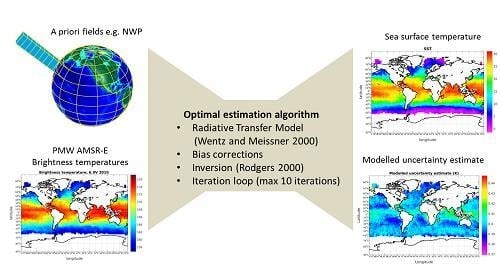
:The Optimal Estimation (OE) technique is developed within the European Space Agency Climate Change Initiative (ESA-CCI) to retrieve subskin Sea Surface Temperature (SST) from AQUA’s Advanced Microwave Scanning Radiometer—Earth Observing System (AMSR-E). A comprehensive matchup database with drifting buoy observations is used to develop and test the OE setup. It is shown that it is essential to update the first guess atmospheric and oceanic state variables and to perform several iterations to reach an optimal retrieval. The optimal number of iterations is typically three to four in the current setup. In addition, updating the forward model, using a multivariate regression model is shown to improve the capability of the forward model to reproduce the observations. The average sensitivity of the OE retrieval is 0.5 and shows a latitudinal dependency with smaller sensitivity for cold waters and larger sensitivity for warmer waters. The OE SSTs are evaluated against drifting buoy measurements during 2010. The results show an average difference of 0.02 K with a standard deviation of 0.47 K when considering the 64% matchups, where the simulated and observed brightness temperatures are most consistent. The corresponding mean uncertainty is estimated to 0.48 K including the in situ and sampling uncertainties. An independent validation against Argo observations from 2009 to 2011 shows an average difference of 0.01 K, a standard deviation of 0.50 K and a mean uncertainty of 0.47 K, when considering the best 62% of retrievals. The satellite versus in situ discrepancies are highest in the dynamic oceanic regions due to the large satellite footprint size and the associated sampling effects. Uncertainty estimates are available for all retrievals and have been validated to be accurate. They can thus be used to obtain very good retrieval results. In general, the results from the OE retrieval are very encouraging and demonstrate that passive microwave observations provide a valuable alternative to infrared satellite observations for retrieving SST.
1. Introduction
Sea surface temperature (SST) is an essential climate variable that is fundamental for climate monitoring, understanding of air–sea interactions, and numerical weather prediction. It has been observed from thermal infrared (IR) satellite instruments since the early 1980s, but these observations are limited by their inability to retrieve SST under clouds and biasing from aerosols [1,2,3]. SST observations from passive microwave (PMW) sensors are widely recognized as an important alternative to the IR observations [4,5]. PMW SST retrievals are not prevented by non-precipitating clouds and the impact of aerosols is small [6,7]. The first PMW SST retrieval algorithm was developed for the Scanning Multichannel Microwave Radiometer (SMMR) on NIMBUS-7 [8,9]. The algorithm used a linear combination of brightness temperatures and the earth incidence angle. It was a two-stage algorithm, first calculating wind speed then selecting the SST regression coefficients if winds were greater than or less than 7 m·s−1. SMMR suffered from significant calibration problems (solar contamination of the hot-load calibration target) that resulted in large errors in the retrieved SST, limiting its usefulness [10].
Since December 1997, a series of satellites have carried well-calibrated PMW radiometers capable of accurately retrieving SST. The first accurate PMW SST data was from the high inclination orbit Tropical Rainfall Measuring Mission (TRMM) Microwave Imager (TMI) that observed equatorward of 40 degrees latitude (limited by the high inclination orbit of the spacecraft and the weak sensitivity of x-band channels (10.65 GHz) at SST less than ~285 K). This was followed in 2002 by the first global PMW SST data from AQUA’s Advanced Microwave Scanning Radiometer—Earth Observing System (AMSR-E) and more recently the follow-on instrument AMSR-2 flown on the Global Change Observing Mission (GCOM-1, e.g., [11]) launched in May 2012. The first spaceborne polarimetric microwave radiometer, WindSat, launched in January 2003, also provides measurements for retrieving SST [12]. These data demonstrated how through-cloud SST measurements offer unique opportunities for research into air–sea interactions, improved coverage in persistently cloudy regions, and could improve the existing operational SST products [6,7,13].
AMSR-E is a partnership, with a JAXA instrument carried on a NASA satellite. Both JAXA and NASA have routinely produced SSTs from AMSR-E; each using different retrieval algorithms developed and refined over years of experience with PMW data. The JAXA algorithm is just focused on producing SST using the 6V channel [14,15]. The NASA algorithm determines SST and wind speed at the same time using a radiative transfer based two-step algorithm [16]. The JAXA AMSR-E SSTs were compared to collocated IR satellite SSTs, for 7 months of data in 2003, and found a 0.0 K mean difference and standard deviation of 0.71/0.60 K for day/night [17]. The NASA AMSR-E SSTs from June 2002 through October 2011 were compared to global drifter SST data, and results showed a mean difference of −0.05 K and standard deviation of 0.48 K [18]. Both products are widely used in the operational ocean and atmospheric modeling communities (e.g., [19]) as well as for scientific research and applications [20,21,22,23].
SST retrievals using the optimal estimation (OE) principle have been developed several years ago for IR retrievals (see e.g., [24,25,26]). The OE retrieval methodology differs from standard regression models, in that it utilizes a forward model that includes a priori information about the ocean and atmospheric state to calculate simulated brightness temperatures. This methodology leads to improvements in the accuracy of IR SST retrievals using OE rather than a Non Linear SST (NLSST) algorithm and was used creating the first IR SST climate data record from the European Space Agency Climate Change Initiative (ESA-CCI) project [24,27]. Although an OE algorithm incurs additional computational costs because of the required forward modeling, it has significant advantages as the optimal estimator can be designed to estimate both retrieval uncertainty and sensitivity [28].
Climate quality global PMW SST retrievals are challenging due to the need to exclude retrievals that include observations from channels affected by wind, atmospheric attenuation and emission, sun-glint, land contamination, and Radio Frequency Interference (RFI). Different groups (e.g., [16,17]) use different exclusion criteria to flag affected data. The use of simulations and the OE methodology for the retrieval is therefore tempting as the algorithm automatically shifts away from the compromised channels and provides additional information which can be used to filter erroneous retrievals.
OE has previously been applied to multi-frequency PMW data [29] and results from AMSR-E retrievals were reported by [30,31]. In these studies, SST was among the retrieved parameters but the focus was to retrieve sea ice parameters. The OE technique has also been applied for WindSat retrievals [32], where SST also was among the retrieved parameters but the focus was on wind vector retrievals. The objective of this study is to develop a retrieval algorithm that provides an optimal and physically consistent retrieval with a specific focus on retrieving SST to be used for generation of a climate data record.
2. Materials and Methods
2.1. Data
2.1.1. AMSR-E Brightness Temperatures
JAXA’s AMSR-E instrument was launched in May 2002 on NASA’s Aqua satellite. The AMSR-E instrument is a conical scanning microwave imaging radiometer that measures both vertical and horizontal linear polarizations at 6.9, 10.7, 18.7, 23.8, 36.5, and 89.0 GHz channels using an antenna diameter of 1.6 m. This suite of channels was chosen to support accurate retrievals of ocean, ice and atmospheric parameters. AMSR-E data are available from June 2002 through October 2011 when the antenna rotating mechanism on the instrument failed. This study uses the spatially resampled L2A swath data product AMSR-E V12 [33], produced by Remote Sensing Systems (RSS) and distributed by NASA’s National Snow and Ice Data Center (NSIDC; https://nsidc.org/data/ae_l2a). The spatial resampling is generated by applying the Backus–Gilbert method to the L1A data. The RSS L2A product includes brightness temperatures for all AMSR-E channels that have been calibrated to the RSS version 7 standard, which includes inter-calibration with other satellite radiometers, and a correction to the AMSR-E hot load used during the calibration [34]. Brightness temperatures are re-sampled to the resolution of other channels and the location where the reflection vector intersects the geostationary sphere, used for development of RFI flagging, is included in the dataset. Sun glint angles are also calculated as a part of the RSS L2A AMSR-E V12 files. For this analysis, we use the re-sampling to 6.9 GHz resolution (75 × 43 km) for the five lowest frequencies.
2.1.2. In Situ Observations
The in situ dataset used for algorithm testing and validation is composed of quality-controlled measurements taken from the International Comprehensive Ocean-Atmosphere Dataset (ICOADS) version 2.5.1 [35], and the Met Office Hadley Centre (MOHC) Ensembles dataset version 4.2.0 (EN4) [36]. Observations from drifting buoys constitute the main source of observations. The temperature sensor on a drifting buoy is placed at around 20 cm depth in calm water, although the depth in perturbed conditions is poorly known. Temperature measurements are typically made hourly with an uncertainty from sensor calibration inferred to be about 0.2 °C [37]. MOHC quality control (QC) flags and track flags are provided with the data. See Atkinson et al. [38] for more information on the quality control.
In addition, temperature observations are used from the Argo profiling floats (see e.g., [39]). The data and quality control of these observations are described in Good et al. [36]. In this study, the uppermost temperature observations from the Argo observations have been used, which have a typical depth of 5 m [40] and a very high accuracy, with uncertainties of 0.002 °C [41,42]. Both Argo and drifting buoy observations have previously been used for algorithm development and validation studies [43,44,45,46].
2.1.3. Ancillary Data Fields
The OE method utilizes a priori information about the state of the ocean and atmosphere as first guess. For this study, we used Numerical Weather Prediction (NWP) information from the ERA-Interim NWP data as first guess on the atmospheric and oceanic state [47]. The ERA-Interim SST fields are from the Operational Sea Surface Temperature and Ice Analysis (OSTIA) level 4 SST analysis, which is generated from IR and PMW satellite observations blended with in situ data from drifting buoys [19,21]. The larger number of IR satellites and the higher spatial resolution compared to the PMW satellite observations means that the OSTIA analysis is dominated by the IR satellite observations. An independent validation showed a global mean difference (OSTIA—Argo floats) of −0.05 K and standard deviation of 0.55 K (see Section 3.3), which was found when the OSTIA SST analysis fields were compared against observations from Argo floats for 2009–2011 (using the data filtering methods described in Section 2.2.2). For Sea Surface Salinity (SSS), we used the monthly, 0.25 degrees spatial resolution, objectively analyzed mean fields, SSS from the World Ocean Atlas (WOA) 2013 version 2 [48,49]. This climatology was determined from historical salinity data from a wide variety of sources that were carefully quality controlled and objectively analyzed into monthly globally complete maps of SSS. These data were linearly interpolated in time and space to the matchup location.
2.2. Matchup Database
2.2.1. ESA-CCI Multi-Sensor Matchup Dataset
The basis for the retrieval algorithmic development and tuning is a Multi-sensor Matchup Dataset (MMD) pioneered by the ESA-CCI SST project [50]. The MMD has been constructed as a general dataset for algorithm development and not specifically for OE development. It includes AMSR-E orbital data matched to in situ measurements (drifting buoys and Argo floats) constrained by a maximally allowed geodesic distance and a maximal time difference.
The MMD was created using a Multi-sensor Matchup System (MMS) software that reads in all the in situ observations and finds the corresponding matching satellite observations throughout the full dataset. Matches were only included within a maximal geodesic distance of 20 km and a time difference of maximally 4 h. The spatial distance ensures that the in situ measurement is located within an AMSR-E footprint. The temporal distance balances the need for accurate collocated data with the need for a large number of useable matches.
The collocated AMSR-E data include a 21 by 21 pixel window with the matchup location in the center as well as all variables of the corresponding in situ measurement. The ERA-Interim NWP data were referenced to each AMSR-E pixel and each in situ measurement and spatially interpolated to the data raster using Climate Data Operators (CDO) [51]. This ancillary information includes a subset of the available ERA-Interim variables, covering a time range of −60 h to +36 h around the matchup time. Processing of the matchup dataset has been performed on the Climate and Environmental Monitoring from Space Facility (CEMS) computing facility at the Centre for Environmental Data Analysis (CEDA).
2.2.2. Data Filtering Methods
Developing an accurate retrieval algorithm relies on the quality of the satellite observations and auxiliary fields used for the retrieval and validation. It is therefore essential to flag erroneous matchups as accurately as possible and produce a clean dataset for the development.
Data have been flagged if any of the following quality flags were set to fail: AMSR-E pixel data quality, AMSR-E scan data quality, MOHC QC flag and MOHC track flag. If the brightness temperature was outside the normal range (0–320 K) for any of the channels, the data were flagged. To discard cases where the atmospheric contribution (largest for the 18–36 GHz channels) exceeds the information from the surface, data were flagged if the difference between the H and V brightness temperatures for the 18–36 GHz channels <0 K (for valid oceanic retrievals V should always be larger than H). Data were also flagged based on the spatial standard deviation of the 23V, 23H, 36V and 36H GHz brightness temperatures in the 21 × 21 pixel extracts surrounding each matchup. If the standard deviation of these channels were higher than 55, 35, 25 and 25 K, respectively, the data were flagged to remove obviously bad observations. Additionally, matchups were excluded if the ancillary data seemed to be erroneous. If in situ or NWP SSTs were less than −2 °C or greater than 40 °C or if NWP wind speeds were greater than 20 m·s−1 then the matchup was flagged. All these flags have been combined into a gross error flag, which in total removes 13.1% of the drifter matchups.
Additional filtering was added to account for various situations where the SST retrieval could be compromised, namely during: land and ice contamination (due to antenna side-lobe contamination), sun glitter contamination, geostationary satellite and ground-based RFI, diurnal warming, and rain contamination. To avoid contamination due to land and ice, the AMSR-E land/ocean flag and NWP sea ice fraction were used to flag data. Applying this filter alone resulted in a flagging of 13.1% of the drifter matchups, which had already passed the gross error check. To avoid sun glitter contamination, data with sun glint angle <25° were flagged (9.6%). Potential contamination due to RFI was detected using the observation location (for ground based RFI) and reflection vector (for geo-stationary RFI) using Table 2 presented in Gentemann et al. [52] (6.5%). To avoid diurnal warming effects, daytime data with NWP wind speeds <4 m·s−1 were flagged (8.0%). Rain contamination was accounted for by flagging data if the brightness temperature of the 18V channel >240 K (0.4%). Applying all these checks at once leads to an elimination of 41.1% of the total drifter matchups.
Finally, to obtain a more equal latitudinal distribution of the drifter matchups, a limit of 40,000 matchups per degree of latitude was imposed, removing an additional 12.2% of the drifter matchups. The summary statistics for different steps in the flagging process are shown in Table 1. The outcome is a high-quality, globally representative, final drifter matchup database. The focus for this study is the year 2010, which consists of 3,764,798 filtered drifter matchups that are used in the following.
The final number of matchups per month during 2010 is shown in Figure 1. Figure 2a shows the geographical distribution of the matchups per square kilometer after all checks have been applied. Figure 2b shows the latitudinal distribution of matchups before and after the even-out-by-latitude filter has been applied, where the red line denotes the maximum allowed matchups per latitude.
Several subsets of the filtered drifter matchups have been applied throughout this study. The subsets were randomly selected from the filtered drifter matchups. This approach was chosen to reduce computational efforts and very small effects were seen on the final results, when the size of the subset was increased or reduced.
The matchups with Argo floats are limited to 95,240, prior to quality filtering. The gross error check removes 18.9% of the Argo matchups. Removing matchups contaminated by land/ice, RFI, rain, and diurnal warming effects sums up to a total removal of 39.3%, leaving 57,810 Argo matchups to be used in the following. Due to a more equal latitudinal matchup distribution and the limited number of matchups, the even-out-by-latitude filter has not been applied here. Figure 3a shows the geographical distribution of the Argo matchups per square kilometer and Figure 3b shows the latitudinal distribution of the Argo matchups after all checks have been applied.
2.3. Optimal Estimation Development
The OE method can be used to retrieve geophysical parameters (e.g., SST) from PMW observations [29]. The relationship between the geophysical parameters and the measured brightness temperatures can be generalized to the following expression [53]:
where y is the measurement vector (observed microwave brightness temperatures); F(x) is the non-linear forward model approximating the physics of the measurement, including the surface emissivity and the radiative transfer through the atmosphere [54]; x is the state vector containing the relevant geophysical properties of the ocean and atmosphere; and e is a residual uncertainty term containing uncertainties due to the measurement noise and uncertainties in the forward model.
y = F(x) + e,
The forward model predicts the top-of-atmosphere microwave brightness temperatures that should be measured by the individual channels of a radiometer given knowledge of the relevant geophysical parameters (x) of the ocean and atmosphere. The forward model used in this study is based on the physical surface emissivity and Radiative Transfer Model (RTM) described in Wentz et al. [54]. The RTM consists of an atmospheric absorption model for oxygen, water vapor and cloud liquid water and a sea surface emissivity model that determines the emissivity as a function of SST, SSS, sea surface wind speed and direction. Some components have been adjusted with respect to Wentz et al. [54]. These include the wind directional signal of sea surface emissivity, which has been suppressed as it did not improve the retrievals; and the fact that we only use the V- and H-polarizations for the 5 lower frequencies: 6.9, 10.7, 18.7, 23.8, 36.5 GHz.
The aim of this study is to invert Equation (1) to retrieve the most likely state vector x that can reproduce the observed microwave brightness temperatures, y. In this study, the inversion approach follows the OE technique by Rodgers [53] and we broadly follow his conventions.
In OE, a priori information about the expected mean and covariance of the geophysical parameters can be used to put restrictions on the variances of the estimated geophysical parameters and thereby improve the retrieval. In this case, the prior information is NWP fields as described in Section 2.1.3.
Assuming the forward model is a general function of the state, the measurement + model error has a Gaussian distribution, and there is a prior estimate with a Gaussian uncertainty distribution, the maximum probability state x can be found by minimizing the cost function, J:
where Sϵ is a covariance matrix for the measurement and forward model uncertainties, Sa is the covariances of the a priori state xa (the a priori guess of the ocean and atmospheric state x). The cost function is a measure of the goodness of the fit to both the measurements (first term on the right) and the a priori state (second term on the right) balanced by the inverse of their relative uncertainties (Sϵ and Sa).
In this nonlinear case, Newtonian iteration is a straightforward numerical method for finding the zero gradient of the cost function, J. Using Newtonian iteration, the state x that minimizes the cost function can be found by:
where Sx is the error covariance matrix of the retrieved parameters:
The matrix K expresses the sensitivity of the forward model to a perturbation in the retrieved parameters, i.e., it is a matrix consisting of the partial derivatives of the brightness temperatures in a particular channel with respect to each parameter of the state vector. Due to non-linearity, these partial derivatives need to be computed at each iteration (state).
2.3.1. Initial OE Setup
The measurement vector, y, used in our forward model consists of dual polarization observations (v-pol and h-pol) at the 5 lower frequencies: 6.9, 10.7, 18.7, 23.8, 36.5 GHz. Four geophysical parameters are considered to be the leading terms controlling the observed microwave brightness temperatures in the measurement situation (considering open-ocean only):
where WS is the wind speed, TCWV is the integrated columnar atmospheric water vapor content, TCLW is the integrated (columnar) cloud liquid water content, and SST is the sea surface temperature.
x = [WS, TCWV, TCLW, SST],
The variations of the retrieved geophysical parameters are restricted by the use of a priori information from NWP about the mean (a priori state) and covariances of the parameters. OE can be considered to be an adjustment of the a priori state vector based on the difference between simulated and observed brightness temperatures. The method takes appropriate account of errors by combining the a priori state vector and the information content in the observed brightness temperatures. The covariance matrix of the geophysical parameters related to x is fixed to:
where = 2 m·s−1, = 0.9 mm, = 1 mm and = 0.50 K. The uncertainties on the WS, TCVW and TCLW are best estimates based upon published validation results (see e.g., [47,55,56,57,58]). The SST uncertainty is derived from a comparison against Argo drifting buoys, using the MMD (see Section 3.3). The measurement covariance matrix, Sϵ is initially set to a diagonal matrix with all diagonal elements equal to 0.1 K [54]. The retrieved state vector is obtained by performing the Newtonian iteration, as described in Equation (3).
2.3.2. Testing for Convergence
For each iteration, the quality can be assessed by comparing the simulated and observed brightness temperatures and requiring these to be consistent within a certain uncertainty. This idea is quantified by the root-mean-square error (RMSETB):
which is a confidence indicator of how well the simulated brightness temperatures, TBcalc fit the observed ones, TBobs. The RMSETB criteria is chosen here over e.g., χ2 as it provides an almost linear relationship with the performance of the OE, which will be shown in Section 3. Figure 4a illustrates the mean RMSETB difference for each iteration using a subset of the drifter MMD. The uncertainty bars mark one standard deviation. A strong reduction in RMSETB and standard deviation is found by performing the first iteration. The second iteration similarly leads to a decrease in RMSETB and standard deviation, while the following iterations show no significant improvement on the mean RMSETB. The usefulness of RMSETB as a confidence indicator will be further illustrated in Section 3.
To reduce computational cost, a convergence analysis is performed to decide whether a retrieval process has converged to sufficient precision or if further iterations are required. According to Rodgers [53] the most straightforward convergence test is to ensure that the cost function (Equation (2)) is actually being minimized. The change in the cost function between two subsequent iterations will always be small near a cost minimum. Noting that the expected value of the cost function at the minimum is equal to m degrees of freedom (m = 10) an appropriate test would be to require the change between iterations of or . In addition, is required to be positive at the final solution.
A maximum of 10 iterations are allowed and a failure to meet the above convergence criterion within 10 iterations leads to an exclusion of the data (<0.1%). Figure 4b shows the number of iterations performed for all drifter matchups during 2010 by applying the convergence criterion. Usually, convergence is reached by iteration 3–4. This setup will be referred to as the initial optimal estimator.
2.3.3. Improving the Forward Model
The PMW observations in the 6–10 GHz observe the subskin SSTs at ~1 mm depth, which is different from the IR skin SST observations where a cool skin effect is included [59]. For conditions free of diurnal variability signals, which is the case for the filtered MMD used here, we can assume that the PMW observed subskin SSTs are similar to the in situ drifting buoy observations at the nominal depth of ~20 cm [23]. We can thus use the in situ observations from the drifting buoys to validate the algorithm and for improving the forward model. Similarly, we can assume that the OSTIA SST fields, which are foundation temperatures, are similar to the subskin SSTs and the SSTs at 20 cm.
The OE method assumes an unbiased prior and forward model, which is not necessarily the case. The comparison against Argo SSTs has already addressed the bias in the prior NWP SST field with a mean difference of −0.05 K, which has been adjusted for. In order to get a measure of the forward model deficiency, we compare TBcalc with TBobs. If we assume optimal forward model input variables and unbiased TBobs, we can regard the TBobs–TBcalc differences as inefficiencies in the forward model that we would like to correct for. In other words, we want to use the best available input variables. Therefore, retrieved WS, TCWV and TCLW and in situ SST values are used in the forward model calculations, to bring us as close to true oceanic and atmospheric conditions as possible. The retrieved variables are obtained by running the initial optimal estimator for a subset of 37,242 matchups. These input variables are used to run the forward model once and the difference TBobs–TBcalc is calculated for each channel. Part of the observed channel biases may be a result of the difference between the RTM used here and the one used in calibration of the RSS L2A product [60]. In addition, the RTM used here, does not include wind directional effects. Following Merchant et al. [25] cells with TBobs–TBcalc differences falling outside the range given by the median ±3 robust standard deviations (RSD) in any of our 10 channels are discarded. Furthermore, only matchups that have passed the convergence test (Section 2.3.2) are included. The derived average TBobs–TBcalc differences of the 10 channels range from −0.75 K on 10 GHz H to 0.62 K on 18.7 GHz V and are subsequently used as a constant bias correction of the forward model. In addition to the constant bias correction, an updated error covariance matrix Sϵ is calculated from the TBobs–TBcalc subset. The updated Sϵ used in the following has an average of square root diagonals of 0.20 K, smallest for 10.7 GHz H and 36.5 GHz H (0.09 K) and largest for 6.9 GHz H (0.31 K).
Further steps are taken to improve the forward model used in the retrieval. The updated optimal estimator has been run for the 3,724,216 drifter matchups in 2010. The retrieved WS, TCWV and TCLW values have subsequently been used together with in situ SST to run the forward model once. Similar to the approach used for the constant bias correction, the simulated brightness temperatures are then compared with satellite observations for each channel. To improve the forward model, we use a correction scheme based upon a multivariate regression model. The regression model applies an empirical fit of TBcalc–TBobs to analytic functions of in situ SST, retrieved WS and NWP wind direction relative to the azimuthal look, . The fitting is done on averaged TBcalc–TBobs values for binned data with respect to SST, WS and and with binning intervals of: 1 °C, 2 m·s−1 and 15°, respectively. Only average values from bins with more than 50 members are used when the regression coefficients are determined. Four sinusoidal terms were found to be the most optimal in representing the wind direction biases. The optimal regression model used for the forward model residuals is:
with individual coefficients calculated for each channel. This correction is added to the simulated brightness temperatures individually every time the forward model is called using retrieved SST and WS from the latest iteration.
Figure 5a–d show the average (solid lines) and standard deviation (dashed lines) of the difference TBcalc–TBobs (final iteration) for all channels, and all matchups during 2010, before (black) and after (blue) the empirical bias correction scheme has been applied. Figure 5a indicates a positive bias at high latitudes, no bias at mid-latitudes and a slightly positive bias at the equatorial regions before the empirical bias correction has been applied. The black line of Figure 5b shows an almost linear trend in bias ranging from a positive bias of about 0.5 K in cold waters, no bias at temperatures ~20–25 °C and a slightly positive bias for warmer waters, which is in good agreement with Figure 5a. Figure 5c also reveals a systematic bias in the TBcalc–TBobs difference with the NWP WS before the empirical bias correction is applied. At low wind speeds little bias is present but with increasing wind speeds the bias rapidly becomes larger. Also, the binned statistics reveal a dependency with a positive bias around ° that might be related to wind direction effects not included in the forward model. The bottom plots show the number of matchups in each bin (blue curve) and the cumulative percentage of matchups (red curve).
The blue lines of Figure 5a–d are the updated residuals after the empirical bias correction scheme has been added to TBcalc for all channels, each time the forward model is called. The application of the empirical bias correction improves the behavior of the residuals against each of the four factors by flattening their bias curves and bringing them closer to zero. The standard deviation of the TBcalc–TBobs difference also decreases with the application of the empirical bias correction scheme.
The retrieved parameters have been compared with and without including the empirical bias correction in the retrieval. The distributions are very similar and mean differences between the two retrievals are: −0.02 m·s−1, −0.04 mm and mm for WS, TCWV and TCLW, respectively.
The empirical bias correction of the forward model completes the steps taken towards the final OE setup. The final OE configuration is briefly summarized in Table 2 and Figure 6 illustrates the different processes performed in the final Danish Meteorological Institute (DMI) OE algorithm. First, the algorithm reads in the predefined Sϵ, Sa and values, where is the perturbation used to calculate the Jacobians. The observation loop is started for each satellite observation pixel or matchup by reading the observed brightness temperatures and the first guess values. Thereafter, the iteration process is initiated. For each iteration, the forward model is used to calculate the simulated brightness temperature from the state vector (in the first step: state vector = first guess). Moreover, the Jacobians (K), cost function (J), uncertainty (Sx) and sensitivity (A, Section 3.1) are calculated. The change in the cost function between two iterations is used to test for convergence and a maximum of 10 iterations are allowed. Until convergence is met, the state vector is updated for each iteration step and the iteration continues. When the iteration process is stopped the state vector is saved together with the uncertainties, corresponding averaging kernels and simulated brightness temperatures.
The drifter matchups covering 2010 have been processed and the final OE SST is presented and validated in the following section. Section 3.3 presents the results using the independent observations from Argo floats covering 2009–2011.
3. Results
The DMI OE retrieval scheme has been run with the final configuration described in Section 2.3.3 for the total number of filtered drifter matchups: 3,764,798 for 2010 (Section 2.2.2). The summary statistics of the OE SSTs against drifters are given in Table 3. The retrievals that did not manage to fulfill the convergence criterion described in Section 2.3.2 within the 10 maximum allowed iterations have been eliminated (<0.1%). The OE retrievals that have passed the convergence criterion give SSTs with an initial bias of 0.02 K and a standard deviation of 0.57 K. We have not checked that the retrievals that did pass the convergence test have actually converged to the required solution. This can be done in several ways. One way is to apply a gross error check to throw away cases with unrealistic conditions. These include: (1) temperature conditions outside the accepted range between −2 °C and 35 °C; (2) retrieved wind speeds outside the range 0–30 m·s−1; and (3) retrieved cloud liquid water outside the range: 0–1.5 kg/kg (mass of condensate/mass of moist air). Applying this gross error check removes 9% of the retrievals and reduces the standard deviation to 0.54 K. Another approach is to check that the retrieval is consistent with the satellite observations by evaluating the RMSETB value as described in Section 2.3.2. The practical usefulness of the quality indicator, RMSETB, is shown in Figure 7. All retrievals that have passed the convergence test have been binned with respect to RMSETB with a bin size of 0.1 K. The number of members in each bin is shown in the bottom plot (blue curve) together with the cumulative percentage (red curve). The middle plot displays the binned distribution of OE SST minus drifter SST (with bin size of 1 K) as a function of binned RMSETB, where the color bar is the number of matchups in each bin. The top plot shows the mean (solid) and standard deviation (dashed) of OE SST minus drifter SST as a function of the binned RMSETB statistic. We notice a large increase in scatter as RMSETB increases. This makes the RMSETB-value an efficient indicator of the quality of the OE SST retrieval. Limiting RMSETB to 1 K removes only 8% of the converged retrievals and leaves the remaining 92% with a bias of 0.02 K and standard deviation of 0.51 K. These results reflect that the RMSETB quality indicator provides a better discrimination of quality compared to the gross error check.
Around 64% of converged retrievals have a RMSETB value below 0.5 K and a corresponding bias of 0.02 K and standard deviation of 0.47 K, while 42% have a RMSETB-value less than 0.35 K and a corresponding bias of 0.02 K and standard deviation of 0.45 K. The validation results of the NWP SSTs are included here for reference, but note that drifting buoy observations and PMW observations have already been included in the generation of the NWP fields, as explained earlier. In the following we will only consider the 64% “good” retrievals, which have a corresponding RMSETB < 0.5 K.
Figure 8a,b show global maps of the gridded (with grid size of 5 degrees) mean and standard deviation of OE SST minus drifter SST, respectively, for the 64% best retrievals with a corresponding RMSETB < 0.5 K. The geographical distribution of the mean OE SST minus drifter SST reveals a dependency on latitude, with positive bias at mid-latitudes and negative bias in high latitudes and the equatorial region, likely linked to surface emissivity issues (dependent on wind speed and direction) and atmospheric effects. We notice areas with high standard deviations in e.g., the Gulf Stream Extension, the Kuroshio Current and the Aghulas Retroflection areas. These western boundary current regions are known to be very dynamical with high mesoscale activity and large SST gradients over smaller scales [61,62]. The mesoscale SST gradients will result in enhanced differences when the large (64 × 32 km native instantaneous field of view at 6.9 GHz) satellite footprints are compared with in situ observations. The elevated variability in these regions is therefore not related to the quality of the OE SST retrieval.
Figure 9a,b show the OE SST performance, considering the retrievals with RMSETB < 0.5 K, as a function of binned drifter SST and NWP WS, respectively. The OE SST displays a warm bias for drifter SSTs in the range of 15–25 °C and similar for the small fraction of very high (>28 °C) SSTs. Figure 9b shows that the OE SST has a bias dependency on the NWP WS with a warm bias for low (<6 m·s−1) wind speeds and a cold bias for higher wind speeds.
3.1. SST Sensitivity
One of the benefits of using the OE framework is that it naturally provides several diagnostics for assessing the quality and sensitivity of the retrieval. One of these diagnostics is the averaging kernel matrix, A, which contains the sensitivities of the retrieved parameters to the true state on its diagonal (and cross-sensitivities between parameters on the off-diagonals):
where xt is the true state. If the averaging kernel was equal to the identity matrix the a priori state would have no influence on the retrieved state, which instead would be obtained purely from the information content of the measured brightness temperatures. The mean SST sensitivity for all drifter matchups during 2010 is found to be 0.50 with above OE setup and Figure 10a shows the geographical distribution of SST sensitivity. The SST sensitivity is lowest in high latitudes and increases towards the equatorial region, which is consistent with the fact that TB/ SST is smaller for cold waters (especially for X-band 10.65 GHz channels) [63]. The equatorial region reveals sensitivities of ~0.6 while high latitudes have sensitivities around 0.4. Sensitivities from 0.39 to 0.65 were reported in Gentemann et al. [64] for 0 °C and 30 °C SST, respectively, for an AMSR-E regression type retrieval. In addition, Prigent et al. [63] used simulations to derive channel sensitivities TB/ SST of ~0.3 to 0.6 for the 6 GHz V. These results are in good agreement with the sensitivities obtained here.
3.2. Retrieval Uncertainty
The OE technique offers several options to estimate an uncertainty for each individual retrieval. The OE methodology directly provides an estimate of the retrieval uncertainty, Sx, due to uncertainties in the measurements, forward model, and in the a priori state vector (see Equation (4)). Considering all converged drifter matchups during 2010, the global mean uncertainty is 0.35 K. From Figure 7, it is evident that the quality of the SST retrieval is closely connected to the RMSETB value from the retrieval. For that reason, we have set up an additional uncertainty indicator based on a scaled RMSETB value, using a scaling factor of 0.55. Figure 11 shows the validation results for the uncertainties of the converged matchups, where the actual SST retrieval differences against drifter observations are displayed versus the theoretical uncertainties obtained from the RMSETB values. The dashed line represents the ideal uncertainty under the assumptions that drifting buoys have a total uncertainty of 0.2 K and that the sampling uncertainty is 0.3 K. The point to satellite footprint sampling difference is estimated based on the results in Høyer et al. [44]. It is evident from the figure that there is a good agreement between the observed uncertainty and the modeled uncertainty estimates that are based on the RMSETB and an integrated part of every OE retrieval. The mean modeled uncertainty is estimated to 0.48 K including the in situ and sampling uncertainty. Figure 10b shows the geographical distribution of RMSETB considering the best 64% retrievals with a corresponding RMSETB < 0.5 K.
3.3. Validation against Independent Argo Floats
The validation against drifting buoys favors the NWP SST validation results as the drifting buoys are included in the OSTIA fields. For that reason, the OE retrieval algorithm has also been run for the 57,810 Argo matchups covering the period 2009–2011 (Section 2.2.2). The matchups with Argo floats are fewer than for drifting buoys; however, they are independent and can thus be used to compare the performance of the OE SST and NWP SST. Table 4 shows the validation of the OE SSTs and NWP SSTs against Argo floats for various subsets based on the listed filters. The Argo validation results resemble what was found for the drifting buoy observations with a very clear relation between the RMSETB and the quality of the OE retrieval, and the highest quality OE retrievals performing better than the NWP SSTs. Note that the standard deviation of differences also includes the point to footprint sampling effects that are larger for the OE retrievals than for the NWP, which has an original spatial resolution of 0.05 degrees in latitude and longitude.
Similar to drifters, two uncertainty estimates are given. The OE uncertainty Sx has an average value of 0.35 K, while the modeled estimate has an uncertainty of 0.47 K. The modeled uncertainty is calculated using a scaled RMSETB with a scaling factor of 0.65. The modeled uncertainty has been evaluated for the Argo matchups and the result is shown in Figure 12. The dashed lines represent the ideal uncertainty under the assumptions that Argo floats have an accuracy of 0.002 K [42] and that the sampling uncertainty is 0.3 K [44].
3.4. OE vs. NWP Latitudinal Performance
Overall the OE SST performs similar to the NWP SST when compared to SST from drifters and Argo floats. However, there are regional differences in the performance of the two SST estimates. Figure 13 shows the latitudinal difference in standard deviations of OE and NWP SST compared against the same set of drifters and Argo floats, respectively. The figure shows that the OE SST performs better than NWP SST in both northern and southern mid-latitudes, while NWP SST performs better in the tropics. The latitudinal pattern in the relative performance is remarkably similar for both the drifting buoys and the Argo floats.
4. Discussion
The OE algorithm developed here is an attempt to develop a dedicated SST OE algorithm based on multi-channel microwave radiometer satellite observations. The OE methodology with the integrated forward modeling based on physical properties that provide simulated brightness temperature estimates for every retrieval contains valuable information on pixel level about the quality of the satellite observations. In addition, the OE technique offers a possibility for identifying and discarding RFI information in a very efficient way that is not possible with statistical retrieval methods, such as regression models.
The basis for the OE setup, the development and improvements in the forward model, as well as the validation is the comprehensive MMD that contains all the required fields for a retrieval matched with in situ observations. The MMD is a very powerful tool for algorithm development and makes testing and dependency assessment straightforward. The results presented here demonstrate that updating the state variable through several iterations is crucial for the quality of the retrievals, with a clear reduction in RMSETB for the first two iterations. This approach resembles what is used for OE sea ice concentration retrieval [30,31] but differs from the OE IR SST retrievals, where one inversion is typically performed [24,25]. The need for several iterations is probably a result of the non-linear behavior of the forward model.
The forward model is an essential part of the OE retrievals. The OE performance therefore depends on the performance of the forward model and any deficiencies in the model to simulate the observed brightness temperature will propagate into the retrieval. During development, it was evident that using the MMD to improve the forward model is an essential step. The main improvements in the forward models ability to simulate the observed brightness temperature were found for the wind speed and SST dependency. Using results from a regression model to correct the forward model led to significant improvements in both the bias and the standard deviation between the simulated and observed brightness temperatures.
In the microwave part of the spectrum, several geophysical factors contribute to changes observed by the satellite, such as the ocean state, water vapor and cloud liquid waters etc. [63]. This means that the sensitivity in e.g., the 6 GHz channel to the actual SST variations is not as high as reported for the thermal IR part of the spectrum, where TCLW and TCWV cases are discarded before assessing the sensitivity [65]. In Prigent et al. [63] a regression based retrieval model is used to derive maximum SST sensitivities in the order of 0.65 for the 6 GHz V channel and decreasing for lower SSTs. These results are in good agreement with what we find here, with an overall sensitivity of 0.50 to the true SST. In addition, the global pattern shows a higher sensitivity at lower latitudes with warmer waters, which is also in agreement with the modeled results.
The global validation results with a mean and standard deviation of OE SST minus drifter SST of 0.02 ± 0.47 K for the best 64% of the matchups are very encouraging. These results are comparable or better than the previous validation results for PMW SST retrievals [66,67], which showed a degradation in the SST performance in cold and moist conditions. Similarly, Gentemann [18] reported on a latitudinal and SST dependency in the standard deviations, when compared to drifting buoys. The OE SST performance shows an increase in standard deviations in regions with large mesoscale activity and strong SST gradients. The reason for this is probably the temporal and spatial sampling errors when satellite observations are compared to pointwise in situ observations. Despite an enhanced spatial sampling effect from the larger PMW satellite footprint, the OE SST retrievals perform better than NWP SST in regions with mesoscale activity at both northern and southern mid-latitudes when validated against drifting buoys and Argo floats. In the tropics NWP SST performs better. It is worth to notice the consistency between drifters and Argos.
The algorithm has been developed to retrieve subskin SSTs in conditions not affected by diurnal warming, as these matchups were filtered out. This allowed the use of drifter observations for improving the forward model and for a detailed validation against drifting buoys with a nominal depth of 20 cm and Argo observations at 5 m. SSTs can also be retrieved during daytime conditions with diurnal warming, but accurate validation of the performance in these conditions against in situ would require a model or method for the subskin to 20 cm or 5 m correction.
The OE retrieval provides optimal estimates of four state variables: WS, TCWV, TCLW and SST. The focus in this paper has been on the SST retrieval and on validating this state variable against accurate in situ observations. To validate all state variables against accurate in situ observations is not straightforward for the other variables. A detailed evaluation and validation of the three other parameters are outside the scope of this paper.
The main strength of OE is that it is able to select channels with the most information and provides an independent estimate for the individual retrievals on the uncertainty of the retrievals. The estimated uncertainties were validated against independent in situ observations. The accurate and reliable uncertainty estimates increase the applicability of the SST dataset. A need for very accurate SST retrievals will of course reduce the number of SST retrievals, but a realistic uncertainty estimate guides the users to select the combination of accuracy versus data coverage that is optimal for their application.
5. Conclusions
In this study, the optimal estimation (OE) method has been used to retrieve subskin sea surface temperature (SST) from passive microwave (PMW) satellite observations. The results indicate that the OE SST has an overall bias (OE SST—drifter SST) of 0.02 K and standard deviation of 0.47 K when considering the 64% matchups, where the simulated and observed brightness temperatures are most consistent. The corresponding mean modeled uncertainty is 0.48 K including the in situ and sampling uncertainty. An independent validation against Argo observations shows a mean difference of 0.01 K, standard deviation of 0.48 K and modeled uncertainty of 0.47 K considering the 62% best matchups. The modeled uncertainty estimates, available for each retrieval, have proven to be accurate and reliable, when compared to in situ observations. The main advantage of the OE technique is its capability to provide valuable information on pixel level about the quality of the satellite observations, which can be used directly to identify and discard erroneous retrievals (e.g., contamination from extreme wind, atmospheric attenuation and emission, sun-glint, land/ice, rain and RFI).
Future work on the OE methodology can include more focus on improving the forward model with regard to the other state variables and on the estimation of the Sa and the Sϵ statistical parameters, as these are key parameters in the retrieval process. Alternative forward models could be tested in the retrieval process, but few accurate forward models exist at present that are suitable for use in an OE context. More work should therefore be put into improving the forward models with the aim of PMW OE SST retrievals. In addition, more work could be done on assessing the role of the first guess values and the impact of these observations on the retrieved SSTs. In the present work, we have disregarded observations in the vicinity of sea ice, but considering the results obtained within the ESA-CCI Sea Ice project, a future development could include the development of an integrated ocean and sea ice OE processor, that is able to estimate the sea ice concentration and SST at the same time and thus allowing for PMW SSTs closer to the marginal ice zone.
In the context of developing an SST climate data record, it is important to note that microwave radiometer provides an independent technique to conventional infrared (IR) radiometer satellite retrievals, potentially adding robustness to the resulting multi-mission satellite SST record. Furthermore, as some areas of the global ocean are quasi-permanently obscured by clouds, few IR measurements are available: microwave radiometry mitigates this negative situation meaning that multi-mission SST datasets provide a better representation of the SST with close to daily coverage with a single wide swath satellite instrument. We note that the GCOM-W AMSR-2 is now continuing the legacy of AMSR-E with an improved capability until the early 2020’s. The rotating joint for the antenna scan mechanism of AMSR-E degraded within ~9.5 years of launch. The design lifetime of AMSR-2 was 5 years so a replacement is urgently needed. However, there is currently no follow-on mission either planned or in development to provide continuity of the 6–7 GHz frequency imaging capability that is fundamental for the retrieval of SST from microwave satellite radiometry. In future, we strongly advocate that the following issues are urgently addressed:
- That the future 6–7 GHz frequency wide swath imaging capability currently provided by GCOM-W AMSR-2 is sustained by flying a new mission. This implies immediate initiation of satellite development for a potential launch in 2025.
- That the spatial resolution of the 6–7 GHz frequency channels is significantly improved to provide a ~10 km native instantaneous spatial resolution (which may imply using a large 6–9 m rotating deployable mesh antenna). This is required to minimize significant loss of data in the coastal zone and marginal sea ice zone due to side lobe contamination, currently there are no valid measurements within 100 km of these areas.
- That the radiometric quality of future satellite microwave radiometers is significantly improved over current capability. This is required because in many areas imaging microwave radiometer measurements are the only measurements available for the SST climate data record in areas characterized by quasi-permanent cloud cover that confounds thermal IR satellite SST retrievals.
- That appropriate combination with one or more higher-frequency channels (10, 18, 37 GHz) is provided in order to resolve the ambiguities in the microwave measurements if too few channels are available.
In terms of current capability, we conclude that overall, the OE SST retrieval results for AMSR-E are very promising and demonstrate that the OE algorithm is complementary to the standard SST retrieval algorithms that are available today.
Acknowledgments
This study was funded as part of the ESA-CCI SST. The MMS was developed under the ESA-CCI and the FIDUCEO project Horizon 2020 research and innovation program under grant agreement No 638822. We thank Christopher J. Merchant for providing valuable inputs and comments to this article.
Author Contributions
Pia Nielsen-Englyst, Jacob L. Høyer, and Leif Toudal Pedersen conceived and designed the experiments. Pia Nielsen-Englyst and Jacob L. Høyer performed the experiments. Pia Nielsen-Englyst, Jacob L. Høyer, Leif Toudal Pedersen, Chelle L. Gentemann, and Craig Donlon analyzed the data. Tom Block developed the matchup database. Emy Alerskans and Chelle L. Gentemann developed the data filtering methods.
Conflicts of Interest
The authors declare no conflict of interest. The founding sponsors had no role in the design of the study; in the collection, analyses, or interpretation of data; in the writing of the manuscript, or in the decision to publish the results.
References
- Vázquez-Cuervo, J.; Armstrong, E.M.; Harris, A. The effect of aerosols and clouds on the retrieval of infrared sea surface temperatures. J. Clim. 2004, 17, 3921–3933. [Google Scholar] [CrossRef]
- Reynolds, R.W. Impact of mount pinatubo aerosols on satellite-derived sea surface temperatures. J. Clim. 1993, 6, 768–774. [Google Scholar] [CrossRef]
- Reynolds, R.W.; Rayner, N.A.; Smith, T.M.; Stokes, D.C.; Wang, W. An improved in situ and satellite sst analysis for climate. J. Clim. 2002, 15, 1609–1625. [Google Scholar] [CrossRef]
- Donlon, C.; Rayner, N.; Robinson, I.; Poulter, D.J.S.; Casey, K.S.; Vazquez-Cuervo, J.; Armstrong, E.; Bingham, A.; Arino, O.; Gentemann, C.; et al. The global ocean data assimilation experiment high-resolution sea surface temperature pilot project. Bull. Am. Meteorol. Soc. 2007, 88, 1197–1213. [Google Scholar] [CrossRef]
- Donlon, C.J.; Casey, K.S.; Gentemann, C.L.; Harris, A. Successes and challenges for the modern sea surface temperature observing system. In Proceeding of OceanObs’09: Sustained Ocean Observations and Information for Society; Hall, J., Harrison, D.E., Stammer, D., Eds.; ESA Publication WPP-306: Venice, Italy, 2010; Volume 2. [Google Scholar]
- Wentz, F.J.; Gentemann, C.; Smith, D.; Chelton, D.B. Satellite measurements of sea surface temperature through clouds. Science 2000, 288, 847–850. [Google Scholar] [CrossRef] [PubMed]
- Chelton, D.B.; Wentz, F.J. Global microwave satellite observations of sea surface temperature for numerical weather prediction and climate research. Bull. Am. Meteorol. Soc. 2005, 86, 1097–1115. [Google Scholar] [CrossRef]
- Wilheit, T.T.; Chang, A.T.C. An algorithm for retrieval of ocean surface and atmospheric parameters from the observations of the scanning multichannel microwave radiometer. Radio Sci. 1980, 15, 525–544. [Google Scholar] [CrossRef]
- Lipes, R.G. Description of SEASAT radiometer status and results. J. Geophys. Res. 1982, 87. [Google Scholar] [CrossRef]
- Milman, A.S.; Wilheit, T.T. Sea surface temperatures from the scanning multichannel microwave radiometer on Nimbus 7. J. Geophys. Res. 1985, 90. [Google Scholar] [CrossRef]
- Maeda, T.; Taniguchi, Y.; Imaoka, K. GCOM-W1 AMSR2 Level 1R Product: Dataset of brightness temperature modified using the antenna pattern matching technique. IEEE Trans. Geosci. Remote Sens. 2016, 54, 770–782. [Google Scholar] [CrossRef]
- Gaiser, P.W.; St Germain, K.M.; Twarog, E.M.; Poe, G.A.; Purdy, W.; Richardson, D.; Grossman, W.; Jones, W.L.; Spencer, D.; Golba, G.; et al. The WindSat spaceborne polarimetric microwave radiometer: Sensor description and early orbit performance. IEEE Trans. Geosci. Remote Sens. 2004, 42, 2347–2361. [Google Scholar] [CrossRef]
- Xie, S.-P. Satellite observations of cool ocean—Atmosphere interaction*. Bull. Am. Meteorol. Soc. 2004, 85, 195–208. [Google Scholar] [CrossRef]
- Shibata, A. Calibration of AMSR-E SST toward a monitoring of global warming. In Proceedings of the 2005 IEEE International Geoscience and Remote Sensing Symposium, Seoul, Korea, 29 July 2005. [Google Scholar]
- Shibata, A. Features of ocean microwave emission changed by wind at 6 GHz. J. Oceanogr. 2006, 62, 321–330. [Google Scholar] [CrossRef]
- Wentz, F.J.; Meissner, T. AMSR_E Ocean Algorithms; Remote Sensing Systems: Santa Rosa, CA, USA, 2007; p. 6. [Google Scholar]
- Hosoda, K.; Murakami, H.; Shibata, A.; Sakaida, F.; Kawamura, H. Difference characteristics of sea surface temperature observed by GLI and AMSR aboard ADEOS-II. J. Oceanogr. 2006, 62, 339–350. [Google Scholar] [CrossRef]
- Gentemann, C.L. Three way validation of MODIS and AMSR-E sea surface temperatures. J. Geophys. Res. Oceans 2014, 119, 2583–2598. [Google Scholar] [CrossRef]
- Donlon, C.J.; Martin, M.; Stark, J.; Roberts-Jones, J.; Fiedler, E.; Wimmer, W. The Operational Sea Surface Temperature and Sea Ice Analysis (OSTIA) system. Remote Sens. Environ. 2012, 116, 140–158. [Google Scholar] [CrossRef]
- Hosoda, K.; Kawamura, H.; Sakaida, F. Improvement of New Generation Sea Surface Temperature for Open ocean (NGSST-O): A new sub-sampling method of blending microwave observations. J. Oceanogr. 2015, 71, 205–220. [Google Scholar] [CrossRef]
- Stark, J.D.; Donlon, C.J.; Martin, M.J.; McCulloch, M.E. OSTIA : An operational, high resolution, real time, global sea surface temperature analysis system. In Proceedings of the OCEANS, Aberdeen, UK, 18–21 June 2007; pp. 1–4. [Google Scholar]
- Reynolds, R.W.; Smith, T.M.; Liu, C.; Chelton, D.B.; Casey, K.S.; Schlax, M.G. Daily high-resolution-blended analyses for sea surface temperature. J. Clim. 2007, 20, 5473–5496. [Google Scholar] [CrossRef]
- Donlon, C.; Casey, K.; Robinson, I.; Gentemann, C.; Reynolds, R.; Barton, I.; Arino, O.; Stark, J.; Rayner, N.; LeBorgne, P.; et al. The GODAE high-resolution sea surface temperature pilot project. Oceanography 2009, 22, 34–45. [Google Scholar] [CrossRef]
- Merchant, C.J.; Le Borgne, P.; Marsouin, A.; Roquet, H. Optimal estimation of sea surface temperature from split-window observations. Remote Sens. Environ. 2008, 112, 2469–2484. [Google Scholar] [CrossRef]
- Merchant, C.J.; Le Borgne, P.; Roquet, H.; Marsouin, A. Sea surface temperature from a geostationary satellite by optimal estimation. Remote Sens. Environ. 2009, 113, 445–457. [Google Scholar] [CrossRef]
- Merchant, C.J.; Embury, O. Simulation and Inversion of Satellite Thermal Measurements. In Experimental Methods in the Physical Sciences; Elsevier: Amsterdam, The Netherlands, 2014; Volume 47, pp. 489–526. ISBN 978-0-12-417011-7. [Google Scholar]
- Merchant, C.J.; Embury, O.; Roberts-Jones, J.; Fiedler, E.; Bulgin, C.E.; Corlett, G.K.; Good, S.; McLaren, A.; Rayner, N.; Morak-Bozzo, S.; et al. Sea surface temperature datasets for climate applications from Phase 1 of the European Space Agency Climate Change Initiative (SST CCI). Geosci. Data J. 2014, 1, 179–191. [Google Scholar] [CrossRef]
- Merchant, C.J.; Le Borgne, P.; Roquet, H.; Legendre, G. Extended optimal estimation techniques for sea surface temperature from the Spinning Enhanced Visible and Infra-Red Imager (SEVIRI). Remote Sens. Environ. 2013, 131, 287–297. [Google Scholar] [CrossRef]
- Pedersen, L.T. Merging microwave radiometer data and meteorological data for improved sea ice concentrations. EARSeL Adv. Remote Sens. 1994, 3, 81–89. [Google Scholar]
- Melsheimer, C.; Heygster, G.; Mathew, N.; Toudal Pedersen, L. Retrieval of sea ice emissivity and integrated retrieval of surface and atmospheric parameters over the Arctic from AMSR-E data. J. Remote Sens. Soc. Jpn. 2009, 29, 236–241. [Google Scholar]
- Scarlat, R.C.; Heygster, G.; Pedersen, L.T. Experiences with an Optimal estimation algorithm for surface and atmospheric parameter retrieval from passive microwave data in the arctic. IEEE J. Sel. Top. Appl. Earth Obs. Remote Sens. 2017, 10, 3934–3947. [Google Scholar] [CrossRef]
- Bettenhausen, M.H.; Smith, C.K.; Bevilacqua, R.M.; Wang, N.Y.; Gaiser, P.W.; Cox, S. A nonlinear optimization algorithm for WindSat wind vector retrievals. IEEE Trans. Geosci. Remote Sens. 2006, 44, 597–610. [Google Scholar] [CrossRef]
- Ashcroft, P.; Wentz, F.J. AMSR-E/Aqua L2A Global Swath Spatially-Resampled Brightness Temperatures (Tb), Version 3. 2013. Available online: https://cmr.earthdata.nasa.gov/search/concepts/C190757121-NSIDC_ECS.html (accessed on 30 July 2016).
- Wentz, F.J. SSM/I Version-7 Calibration Report; Remote Sensing Systems: Santa Rosa, CA, USA; 2013; p. 46. [Google Scholar]
- Woodruff, S.D.; Worley, S.J.; Lubker, S.J.; Ji, Z.; Eric Freeman, J.; Berry, D.I.; Brohan, P.; Kent, E.C.; Reynolds, R.W.; Smith, S.R.; et al. ICOADS Release 2.5: Extensions and enhancements to the surface marine meteorological archive. Int. J. Climatol. 2011, 31, 951–967. [Google Scholar] [CrossRef]
- Good, S.A.; Martin, M.J.; Rayner, N.A. EN4: Quality controlled ocean temperature and salinity profiles and monthly objective analyses with uncertainty estimates: THE EN4 DATA SET. J. Geophys. Res. Oceans 2013, 118, 6704–6716. [Google Scholar] [CrossRef]
- O’Carroll, A.G.; Eyre, J.R.; Saunders, R.W. Three-Way Error Analysis between AATSR, AMSR-E, and In Situ sea surface temperature observations. J. Atmos. Ocean. Technol. 2008, 25, 1197–1207. [Google Scholar] [CrossRef]
- Atkinson, C.P.; Rayner, N.A.; Kennedy, J.J.; Good, S.A. An integrated database of ocean temperature and salinity observations. J. Geophys. Res. Oceans 2014, 119, 7139–7163. [Google Scholar] [CrossRef]
- Roemmich, D.; Johnson, G.; Riser, S.; Davis, R.; Gilson, J.; Owens, W.B.; Garzoli, S.; Schmid, C.; Ignaszewski, M. The Argo Program: Observing the Global Oceans with Profiling Floats. Oceanography 2009, 22, 34–43. [Google Scholar] [CrossRef]
- Gille, S.T. Decadal-Scale Temperature Trends in the Southern Hemisphere Ocean. J. Clim. 2008, 21, 4749–4765. [Google Scholar] [CrossRef]
- Kennedy, J.J. A review of uncertainty in in situ measurements and data sets of sea surface temperature: In situ sst uncertainty. Rev. Geophys. 2014, 52, 1–32. [Google Scholar] [CrossRef]
- Abraham, J.P.; Baringer, M.; Bindoff, N.L.; Boyer, T.; Cheng, L.J.; Church, J.A.; Conroy, J.L.; Domingues, C.M.; Fasullo, J.T.; Gilson, J.; et al. A review of global ocean temperature observations: Implications for ocean heat content estimates and climate change: Review of ocean observations. Rev. Geophys. 2013, 51, 450–483. [Google Scholar] [CrossRef]
- Embury, O.; Merchant, C.J.; Corlett, G.K. A reprocessing for climate of sea surface temperature from the along-track scanning radiometers: Initial validation, accounting for skin and diurnal variability effects. Remote Sens. Environ. 2012, 116, 62–78. [Google Scholar] [CrossRef]
- Høyer, J.L.; Karagali, I.; Dybkjær, G.; Tonboe, R. Multi sensor validation and error characteristics of Arctic satellite sea surface temperature observations. Remote Sens. Environ. 2012, 121, 335–346. [Google Scholar] [CrossRef]
- Merchant, C.J.; Embury, O.; Rayner, N.A.; Berry, D.I.; Corlett, G.K.; Lean, K.; Veal, K.L.; Kent, E.C.; Llewellyn-Jones, D.T.; Remedios, J.J.; et al. A 20 year independent record of sea surface temperature for climate from Along-Track Scanning Radiometers: SST for climate from atsrs. J. Geophys. Res. Oceans 2012, 117. [Google Scholar] [CrossRef]
- Udaya Bhaskar, T.V.S.; Rahman, S.H.; Pavan, I.D.; Ravichandran, M.; Nayak, S. Comparison of AMSR-E and TMI sea surface temperature with Argo near-surface temperature over the Indian Ocean. Int. J. Remote Sens. 2009, 30, 2669–2684. [Google Scholar] [CrossRef]
- Dee, D.P.; Uppala, S.M.; Simmons, A.J.; Berrisford, P.; Poli, P.; Kobayashi, S.; Andrae, U.; Balmaseda, M.A.; Balsamo, G.; Bauer, P.; et al. The ERA-Interim reanalysis: configuration and performance of the data assimilation system. Q. J. R. Meteorol. Soc. 2011, 137, 553–597. [Google Scholar] [CrossRef]
- Zweng, M.M.; Reagan, J.R.; Antonov, J.I.; Seidov, D.; Biddle, M.M. World Ocean Atlas 2013, Volume 2, Salinity. 2013. Available online: https://repository.library.noaa.gov/view/noaa/14848 (accessed on 26 June 2017).
- Boyer, T.P.; Antonov, J.I.; Baranova, O.K.; Garcia, H.E.; Johnson, D.R.; Mishonov, A.V.; O’Brien, T.D.; Seidov, D.; Smolyar, I.; Zweng, M.M.; et al. World Ocean Database 2013; NOAA Printing Office: Silver Spring, MD, USA, 2013; 208p. [Google Scholar]
- Block, T.; Embacher, S.; Merchant, C.J.; Donlon, C. High performance software framework for the calculation of satellite-to-satellite data matchups (MMS version 1.2). Geosci. Model Dev. Discuss. 2017, 1–15. [Google Scholar] [CrossRef]
- Schulzweida, U.; Kornblueh, L.; Quast, R. CDO User’s Guide—Climate Data Operators; Max Planck Institute for Meteorology: Hamburg, Germany, 2010; pp. 1–173. [Google Scholar]
- Gentemann, C.L.; Hilburn, K.A. In situ validation of sea surface temperatures from the GCOM-W1 AMSR2 RSS calibrated brightness temperatures: Validation of RSS GCOM-W1 SST. J. Geophys. Res. Oceans 2015, 120, 3567–3585. [Google Scholar] [CrossRef]
- Rodgers, C.D. Inverse Methods for Atmospheric Sounding—Theory and Practice; Series on Atmospheric Ocanic and Planetary Physics; World Scientific Publishing Co. Pte. Ltd.: Singapore, 2000; Volume 2, ISBN 978-981-281-371-8. [Google Scholar]
- Wentz, F.J.; Meissner, T. AMSR Ocean Algorithm. Algorithm Theoretical Basis Document; Remote Sensing Systems: Santa Rosa, CA, USA, 2000. [Google Scholar]
- Chelton, D.B.; Freilich, M.H. Scatterometer-based assessment of 10-m wind analyses from the operational ECMWF and NCEP Numerical weather prediction models. Mon. Weather Rev. 2005, 133, 409–429. [Google Scholar] [CrossRef]
- Jakobson, E.; Vihma, T.; Palo, T.; Jakobson, L.; Keernik, H.; Jaagus, J. Validation of atmospheric reanalyses over the central Arctic Ocean: Tara reanalyses validation. Geophys. Res. Lett. 2012, 39. [Google Scholar] [CrossRef]
- Li, J.-L.F.; Waliser, D.; Woods, C.; Teixeira, J.; Bacmeister, J.; Chern, J.; Shen, B.-W.; Tompkins, A.; Tao, W.-K.; Köhler, M. Comparisons of satellites liquid water estimates to ECMWF and GMAO analyses, 20th century IPCC AR4 climate simulations, and GCM simulations. Geophys. Res. Lett. 2008, 35. [Google Scholar] [CrossRef]
- Jiang, J.H.; Su, H.; Zhai, C.; Perun, V.S.; Del Genio, A.; Nazarenko, L.S.; Donner, L.J.; Horowitz, L.; Seman, C.; Cole, J.; et al. Evaluation of cloud and water vapor simulations in CMIP5 climate models using NASA “A-Train” satellite observations: Evaluation of IPCC Ar5 model simulations. J. Geophys. Res. Amospheres 2012, 117. [Google Scholar] [CrossRef]
- Donlon, C.J.; Minnett, P.J.; Gentemann, C.; Nightingale, T.J.; Barton, I.J.; Ward, B.; Murray, M.J. Toward improved validation of satellite sea surface skin temperature measurements for climate research. J. Clim. 2002, 15, 353–369. [Google Scholar] [CrossRef]
- Meissner, T.; Wentz, F.J. The emissivity of the ocean surface between 6 and 90 GHz over a large range of wind speeds and earth incidence angles. IEEE Trans. Geosci. Remote Sens. 2012, 50, 3004–3026. [Google Scholar] [CrossRef]
- Pascual, A.; Faugère, Y.; Larnicol, G.; Le Traon, P.-Y. Improved description of the ocean mesoscale variability by combining four satellite altimeters. Geophys. Res. Lett. 2006, 33. [Google Scholar] [CrossRef]
- Legeckis, R. A survey of worldwide sea surface temperature fronts detected by environmental satellites. J. Geophys. Res. 1978, 83. [Google Scholar] [CrossRef]
- Prigent, C.; Aires, F.; Bernardo, F.; Orlhac, J.-C.; Goutoule, J.-M.; Roquet, H.; Donlon, C. Analysis of the potential and limitations of microwave radiometry for the retrieval of sea surface temperature: Definition of MICROWAT, a new mission concept: Sea Temperature from Microwaves. J. Geophys. Res. Oceans 2013, 118, 3074–3086. [Google Scholar] [CrossRef]
- Gentemann, C.L.; Meissner, T.; Wentz, F.J. Accuracy of satellite sea surface temperatures at 7 and 11 GHz. IEEE Trans. Geosci. Remote Sens. 2010, 48, 1009–1018. [Google Scholar] [CrossRef]
- Merchant, C.J.; Harris, A.R.; Roquet, H.; Le Borgne, P. Retrieval characteristics of non-linear sea surface temperature from the advanced very high resolution radiometer. Geophys. Res. Lett. 2009, 36. [Google Scholar] [CrossRef]
- Castro, S.L.; Wick, G.A.; Jackson, D.L.; Emery, W.J. Error characterization of infrared and microwave satellite sea surface temperature products for merging and analysis. J. Geophys. Res. 2008, 113. [Google Scholar] [CrossRef]
- Dong, S.; Gille, S.T.; Sprintall, J.; Gentemann, C. Validation of the advanced microwave scanning radiometer for the earth observing system (AMSR-E) sea surface temperature in the southern ocean. J. Geophys. Res. 2006, 111. [Google Scholar] [CrossRef]
Figure 1.
Number of matchups per month.
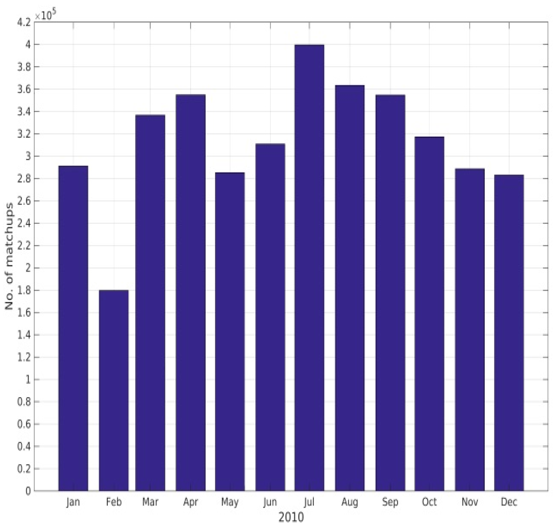
Figure 2.
(a) Geographical distribution of drifter matchups per square kilometer during 2010; (b) the latitudinal distribution of drifter matchups before and after the number of matchups have been evened out by latitude. The red line denotes the maximum allowed matchups per latitude.
Figure 2.
(a) Geographical distribution of drifter matchups per square kilometer during 2010; (b) the latitudinal distribution of drifter matchups before and after the number of matchups have been evened out by latitude. The red line denotes the maximum allowed matchups per latitude.
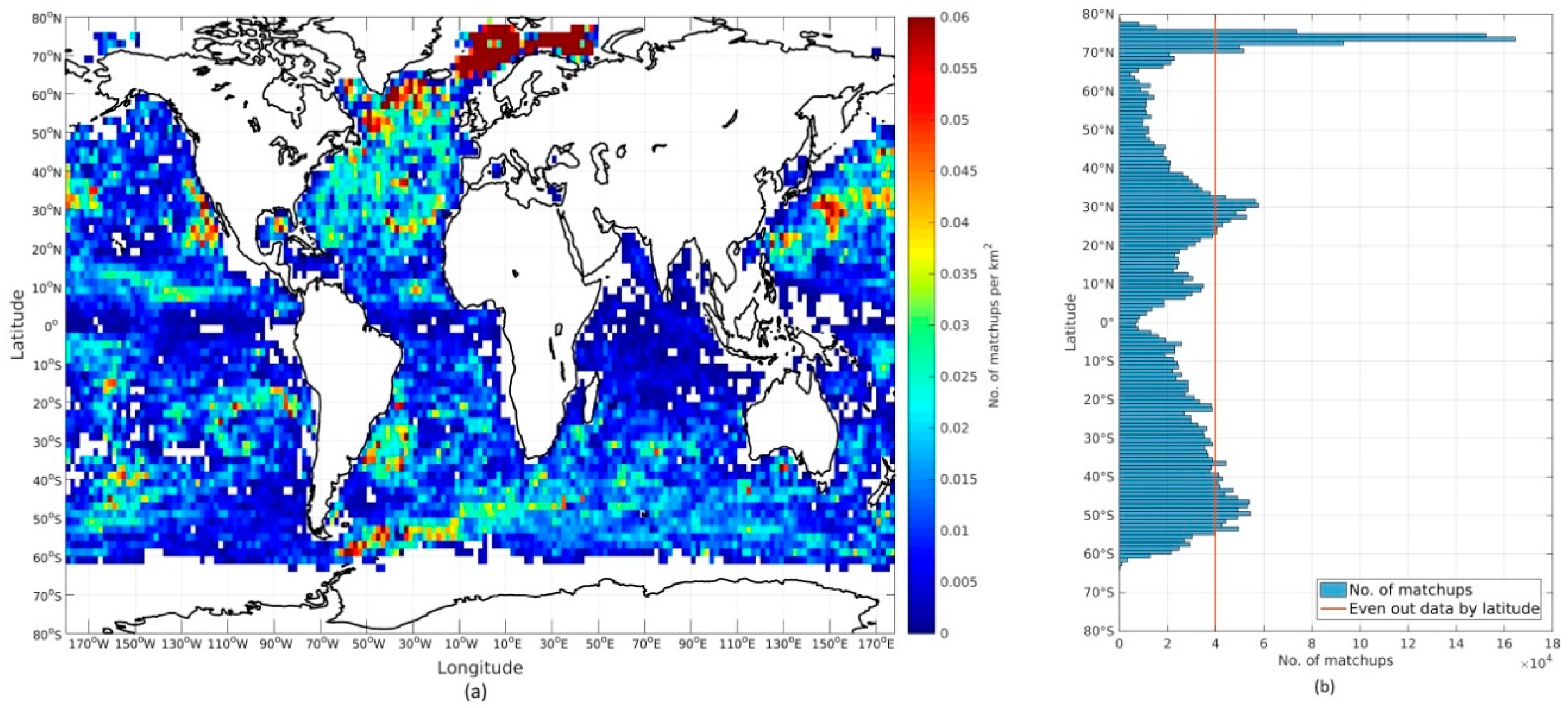
Figure 3.
(a) Geographical distribution of Argo matchups per square kilometer during 2009–2011; (b) the latitudinal distribution of Argo matchups.
Figure 3.
(a) Geographical distribution of Argo matchups per square kilometer during 2009–2011; (b) the latitudinal distribution of Argo matchups.
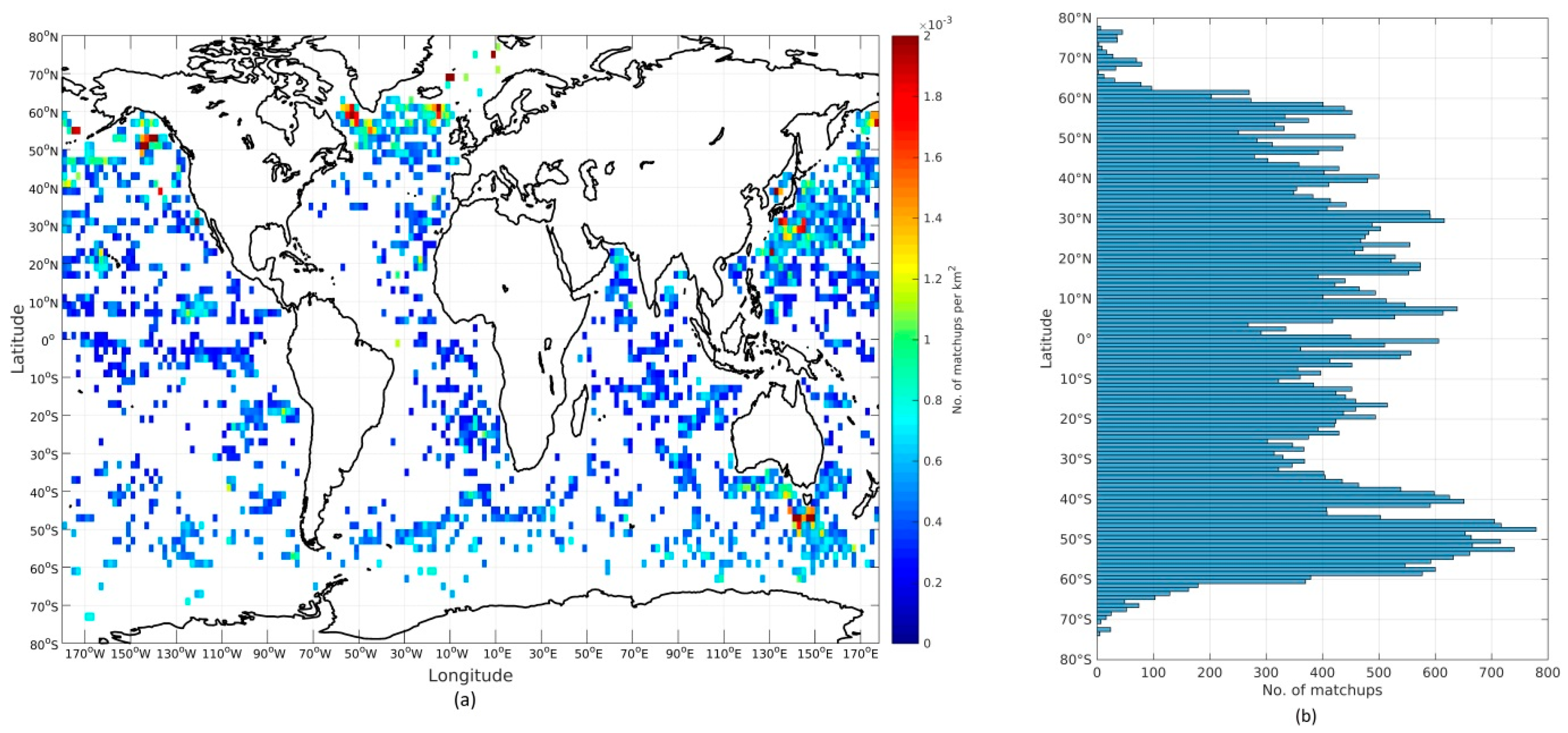
Figure 4.
(a) The mean RMSETB for all channels is plotted for each iteration number. Uncertainty bars show one standard deviation; (b) number of iterations performed for all drifter matchups during 2010.
Figure 4.
(a) The mean RMSETB for all channels is plotted for each iteration number. Uncertainty bars show one standard deviation; (b) number of iterations performed for all drifter matchups during 2010.

Figure 5.
Mean simulated minus observed brightness temperatures for all channels against (a) Latitude; (b) Drifter SST; (c) NWP WS; (d) NWP wind direction relative to azimuthal satellite look. Dashed lines are standard deviations and solid lines are biases. The black and blue colors denote differences before/after the empirical bias correction has been applied. The bottom plots show the number of matchups (blue) and the cumulative percentage of matchups (red) for each data bin.

Figure 6.
Flowchart of the DMI OE algorithm.

Figure 7.
OE SST minus drifter SST as a function of binned RMSETB. The dashed line is standard deviation while the solid line is bias in the upper figure. The surface plot in the middle figure shows the number of matchups in each bin, while the bottom plot shows the number of matchups (blue) and the cumulative percentage of matchups (red) in each RMSETB bin.
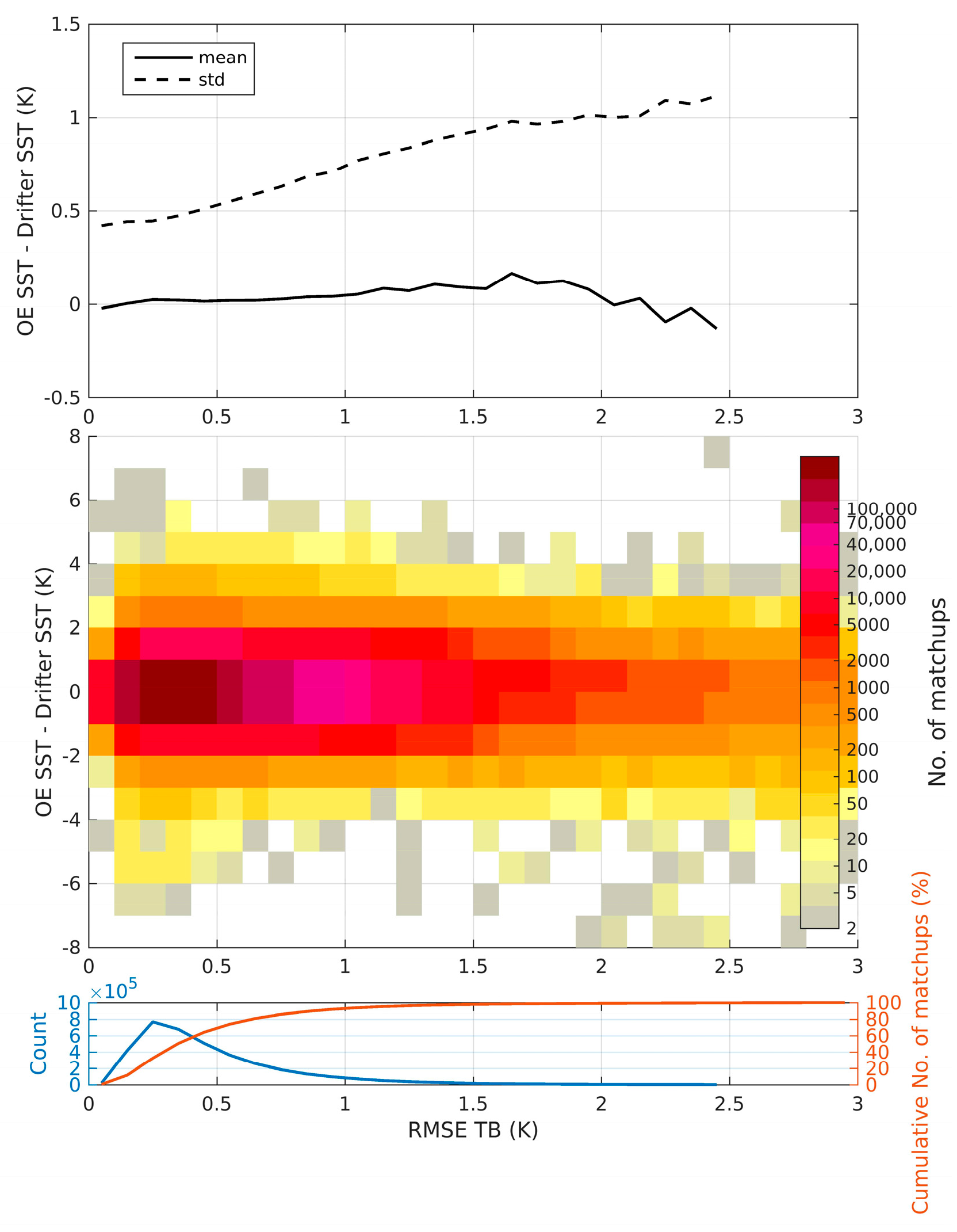
Figure 8.
(a) Mean OE SST minus drifter SST; (b) Mean standard deviation of the OE retrieved minus drifter SST difference. Only retrievals with a corresponding RMSETB < 0.5 K are plotted in the figures.
Figure 8.
(a) Mean OE SST minus drifter SST; (b) Mean standard deviation of the OE retrieved minus drifter SST difference. Only retrievals with a corresponding RMSETB < 0.5 K are plotted in the figures.

Figure 9.
OE SST minus drifter SST as a function of binned (a) Drifter SST; (b) NWP WS. Solid lines are bias and dashed lines are standard deviation in the upper figures. The surface plots in middle figures show the number of matchups in each bin, while the bottom plots show the total number of matchups (blue) and the cumulative percentage of matchups (red) in each drifter SST and NWP WS bin, respectively. Only retrievals with a corresponding RMSETB < 0.5 K are plotted in the figures.

Figure 10.
Gridded statistics of (a) mean sensitivity and (b) mean RMSETB. Only retrievals with a corresponding RMSETB < 0.5 K are plotted.
Figure 10.
Gridded statistics of (a) mean sensitivity and (b) mean RMSETB. Only retrievals with a corresponding RMSETB < 0.5 K are plotted.

Figure 11.
OE SST uncertainty validation with respect to drifter SST. Dashed lines show the ideal uncertainty model accounting for uncertainties in drifter SST and the sampling error. Solid black lines show one standard deviation of the retrieved minus drifter differences for each 0.1 K bin and the red symbols mark the mean bias. The bottom plot shows number of matchups (blue) and the cumulative percentage of matchups for each bin (red).
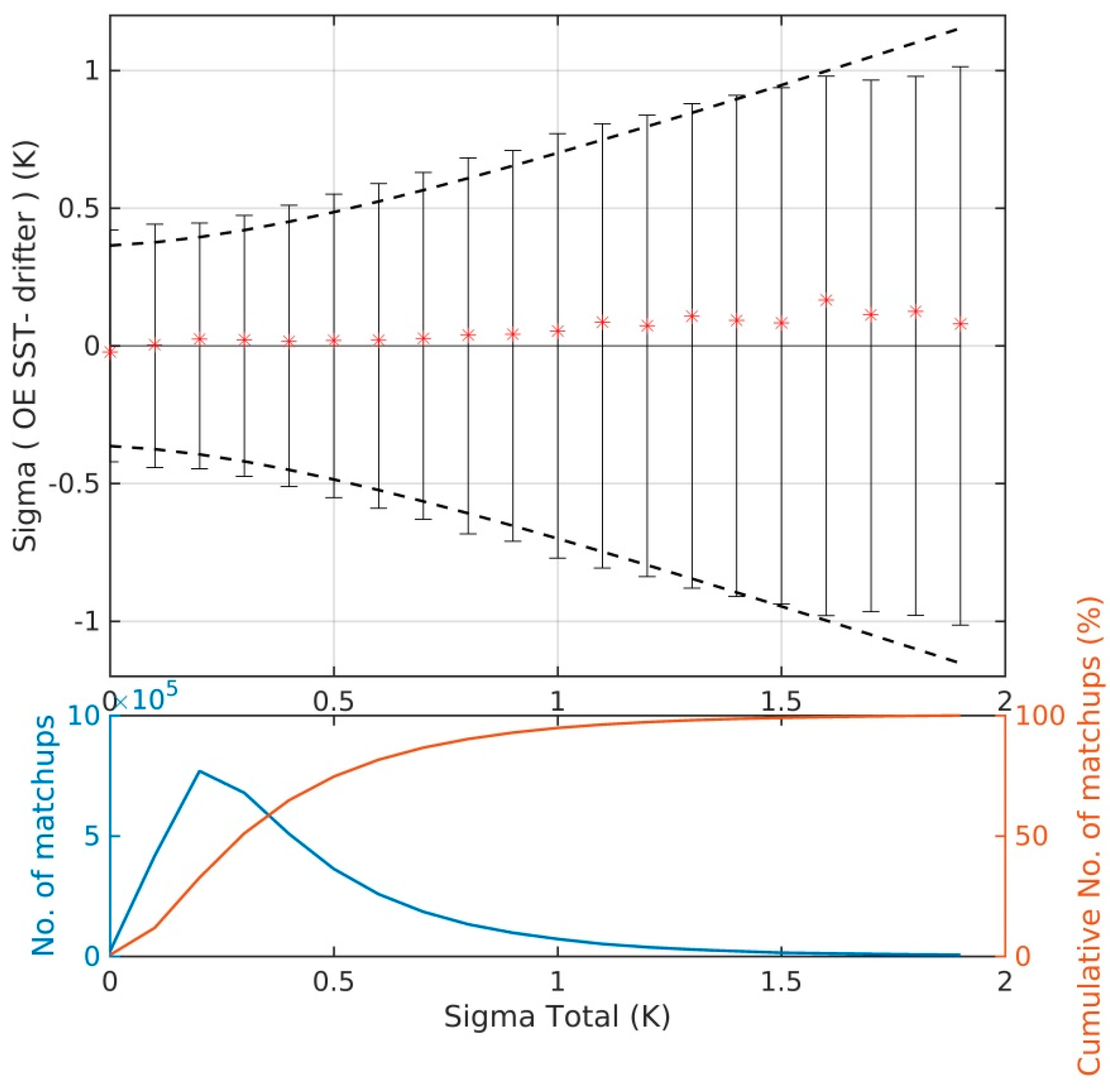
Figure 12.
OE SST uncertainty validation with respect to Argo SSTs. Dashed lines show the ideal uncertainty model accounting for uncertainties in Argo SST and the sampling error. Solid black lines show one standard deviation of the retrieved minus Argo differences for each 0.1 K bin and the red symbols mark the mean bias. The bottom plot shows number of matchups (blue) and the cumulative percentage of matchups (red) for each bin.

Figure 13.
The latitudinal difference in standard deviations of OE and NWP SST compared against in situ SST. The blue curve is the comparison against drifters, while the red curve shows the comparison against Argo floats.
Figure 13.
The latitudinal difference in standard deviations of OE and NWP SST compared against in situ SST. The blue curve is the comparison against drifters, while the red curve shows the comparison against Argo floats.


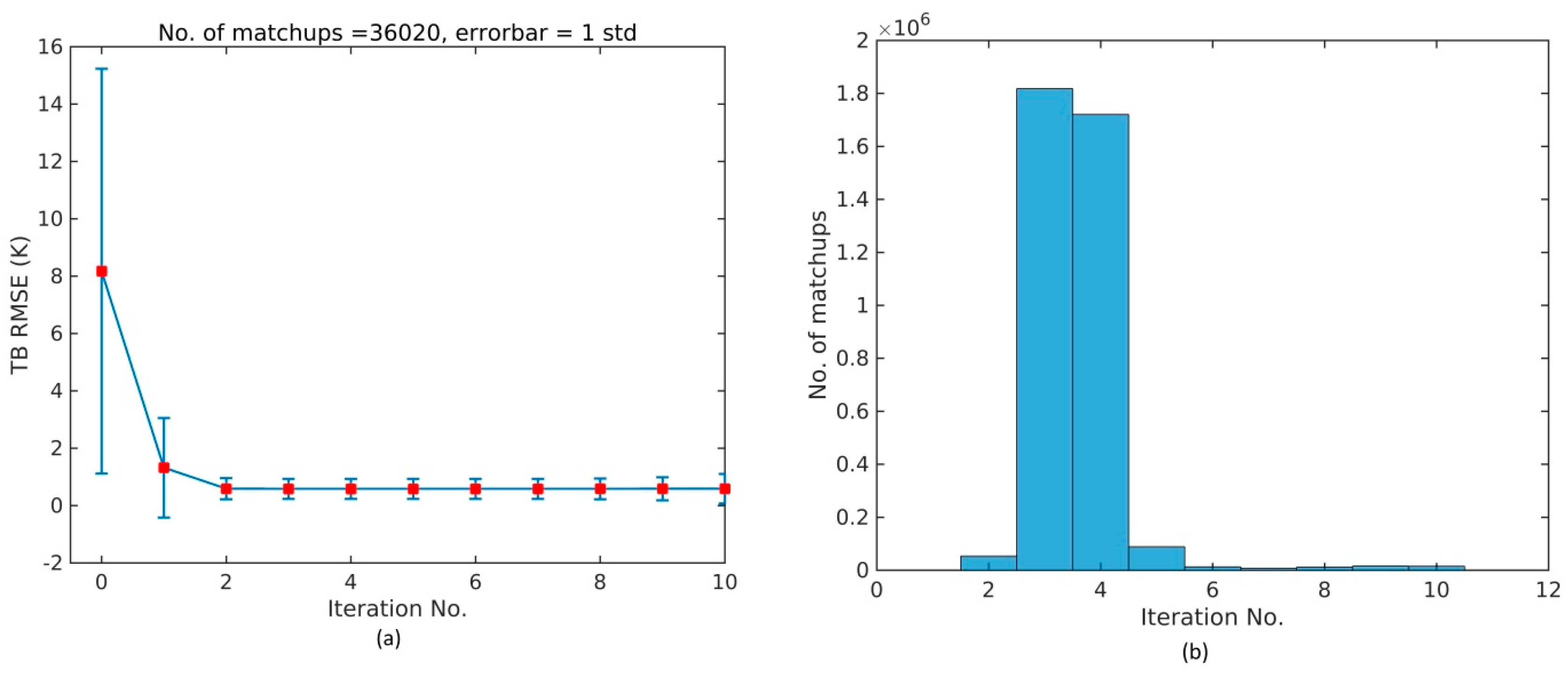
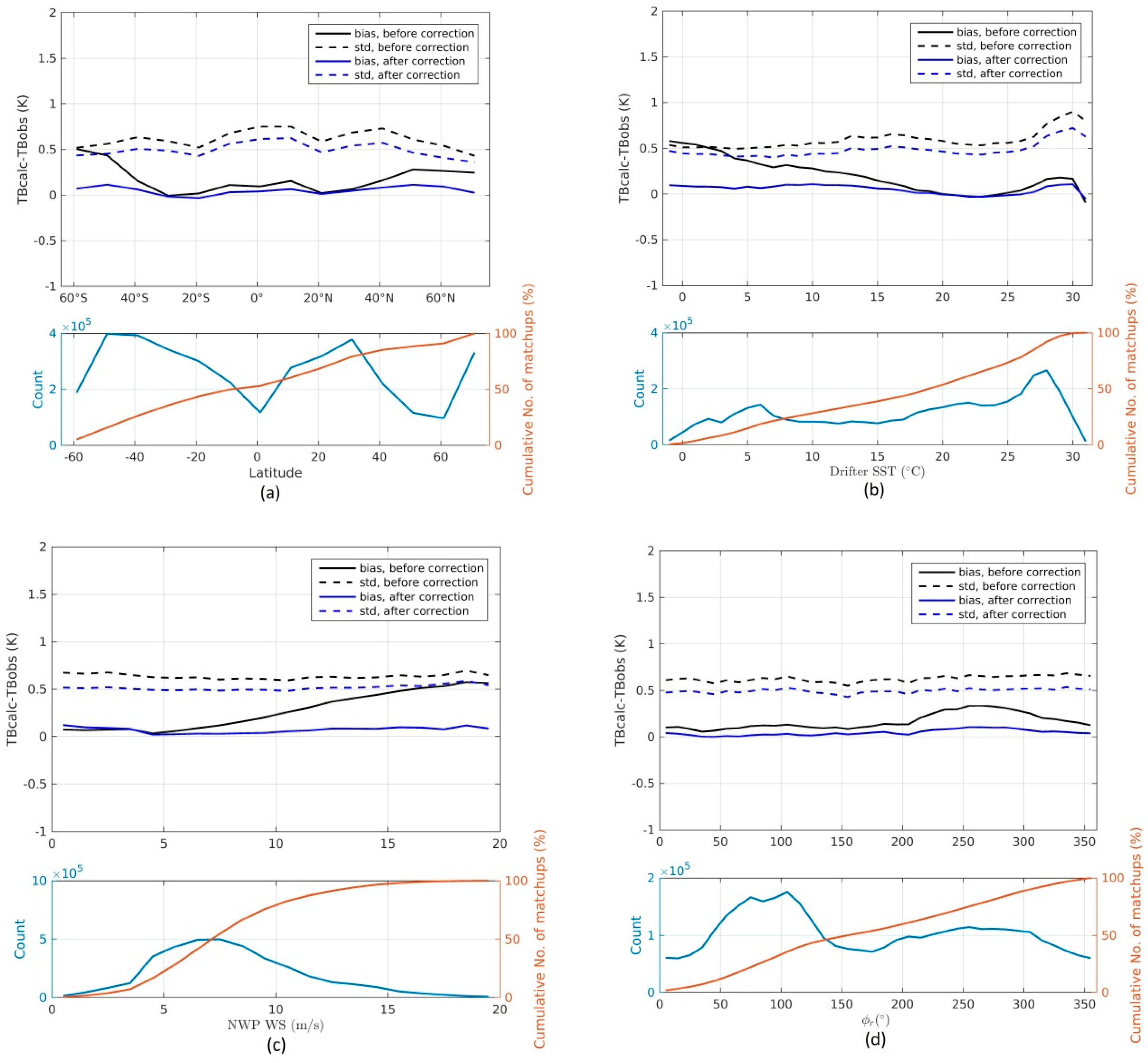
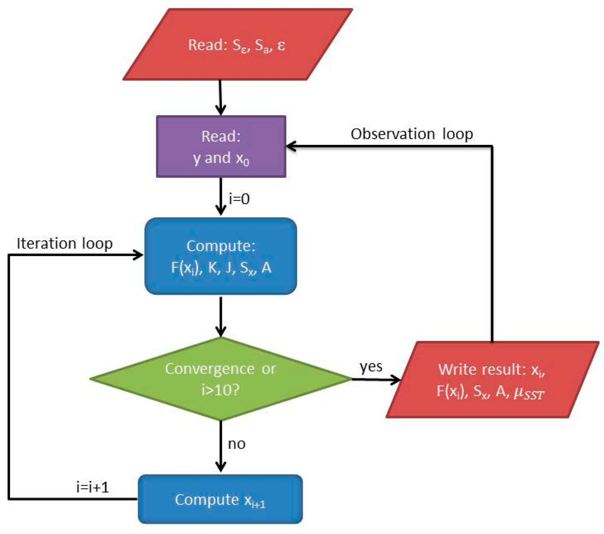
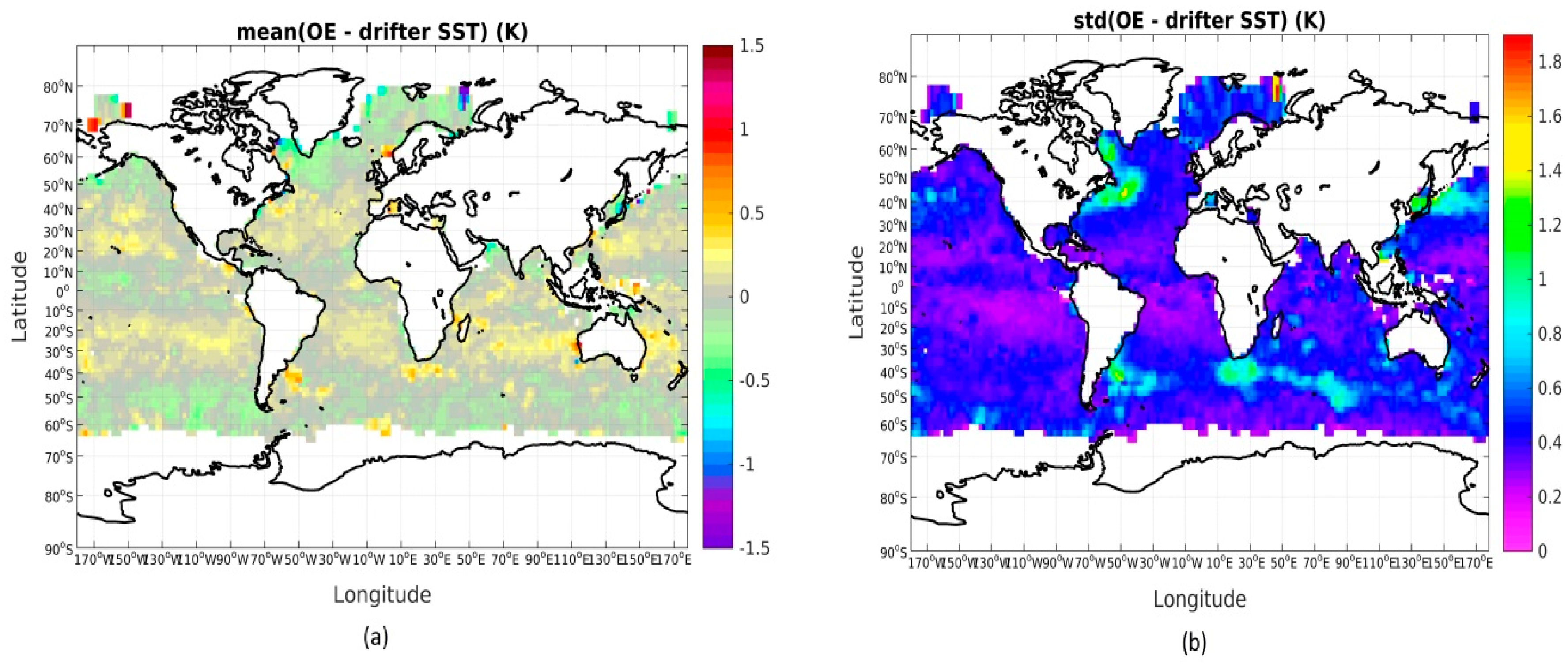
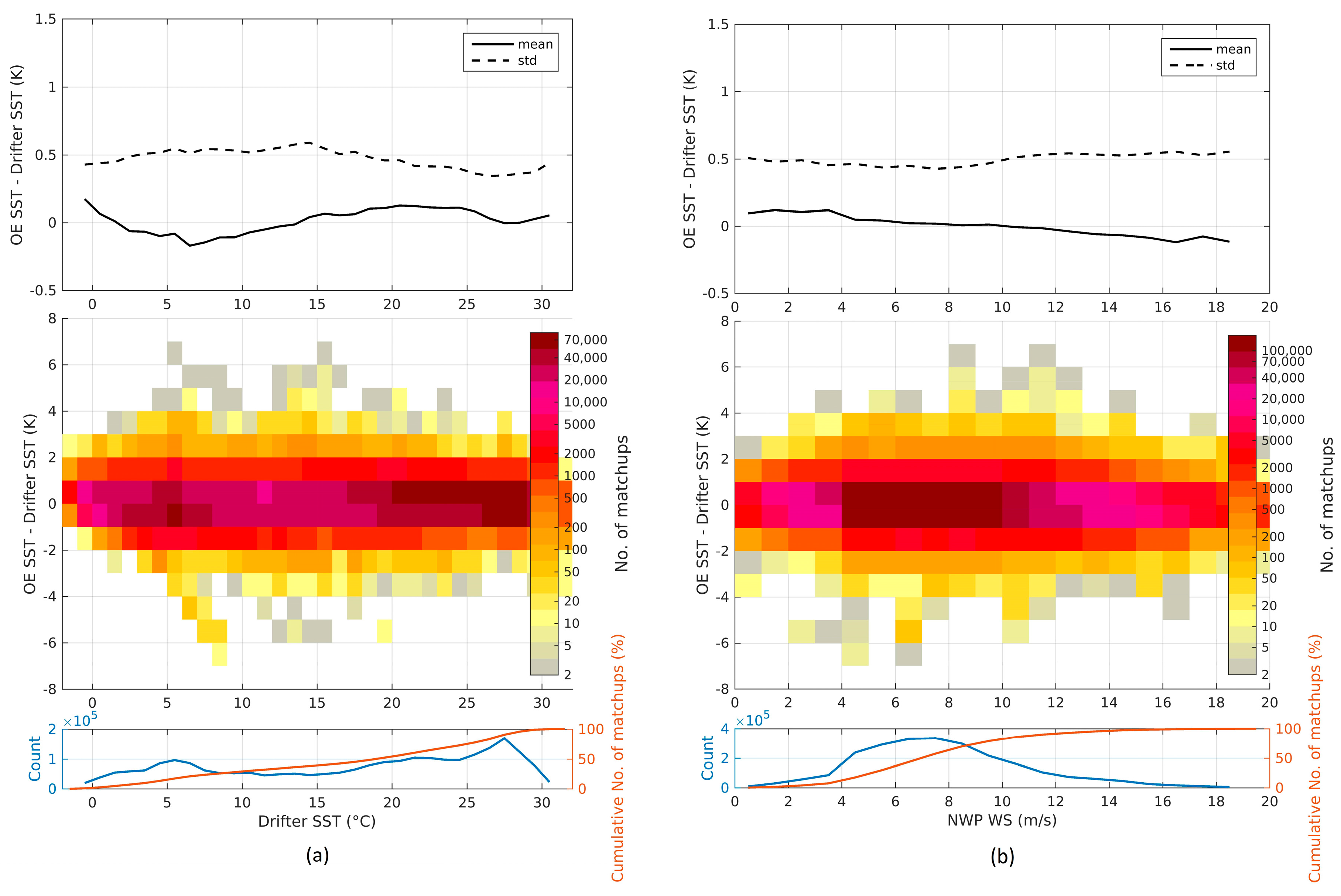
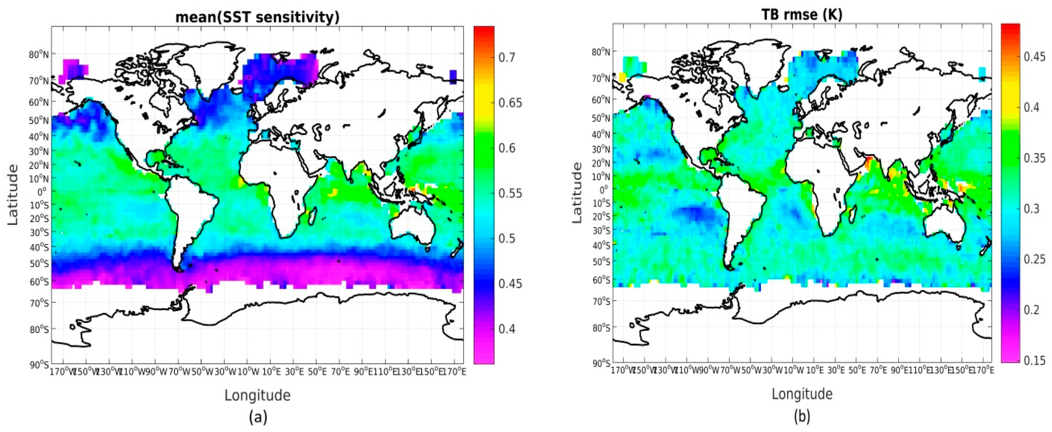
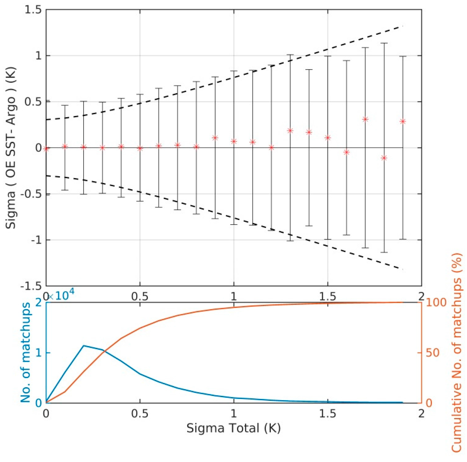
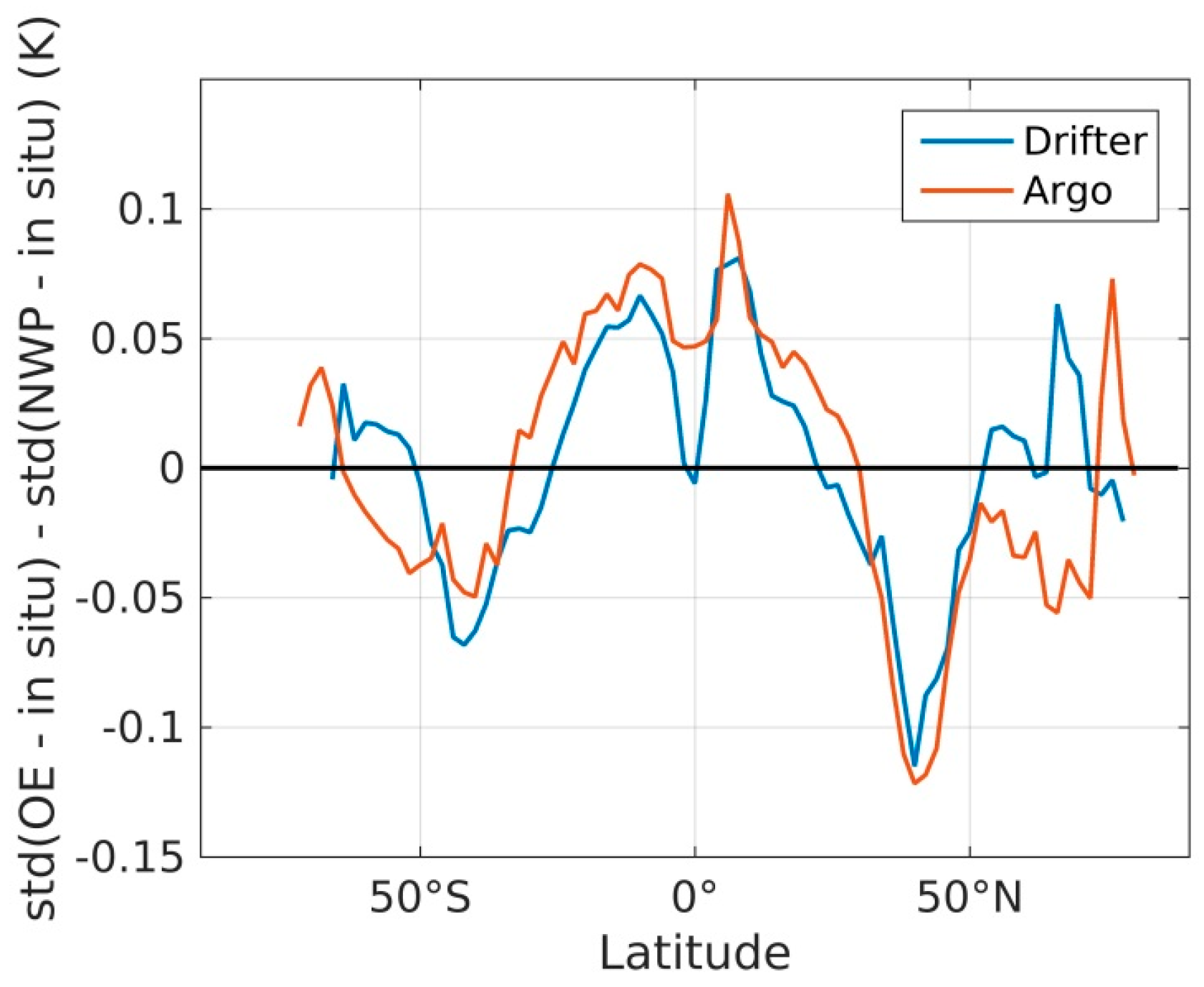
Table 1.
Summary of 2010 data discarded due to the different filters applied.
| Flagging | N | % Removed |
|---|---|---|
| All matchups | 7,278,035 | |
| Gross error flag | 6,323,288 | 13.1 |
| 13.1 | |
| 9.6 | |
| 6.5 | |
| 8.0 | |
| 0.4 | |
| All above checks | 4,286,354 | 41.1 |
| Even out by latitude | 3,764,798 | 12.2 |
| Total | 3,764,798 | 48.3 |
1 Percentage of gross error checked matchups removed by applying each filter individually.
Table 2.
Final optimal estimator configuration.
| Aspect of Optimal Estimator | Configuration |
|---|---|
| Initial forward model, iF(x) | Modified from Wentz et al. [54] (Section 2.3.1) |
| Channels used in retrieval | 6.9, 10.7, 18.7, 23.8, 36.5 GHz (V/H) |
| First guess fields, xa | NWP (Section 2.1.3) |
| Prior error covariance for SST, | 0.5 K |
| Error covariance of observations and model, Sϵ | Full matrix (Section 2.3.2) |
| Convergence criterion | . (Section 2.3.2) |
| IterationsImproved forward model, F(x) | Max iterations = 10iF(x) + corrections (Section 2.3.3) |
Table 3.
Comparison of retrieved SSTs and NWP SSTs against drifter SSTs for various subsets.
| Filter | Bias/K OE-Drifter | std/K OE-Drifter | Bias/K NWP-Drifter | std/K NWP-Drifter | N (106) | |
|---|---|---|---|---|---|---|
| Convergence test passed | 0.02 | 0.57 | −0.04 | 0.50 | 3.7429 | =100% |
| Gross error check | 0.04 | 0.54 | −0.04 | 0.50 | 3.4071 | =91% |
| RMSETB < 1 K | 0.02 | 0.51 | −0.04 | 0.50 | 3.4329 | =92% |
| RMSETB < 0.50 K | 0.02 | 0.47 | −0.04 | 0.48 | 2.3953 | =64% |
| RMSETB < 0.35 K | 0.02 | 0.45 | −0.04 | 0.47 | 1.5681 | =42% |
Table 4.
Comparison of OE SSTs and NWP SSTs against Argo SSTs for various subsets.
| Filter | Bias/K OE-Argo | std/K OE-Argo | Bias/K NWP-Argo | std/K NWP-Argo | N | |
|---|---|---|---|---|---|---|
| Convergence test passed | 0.01 | 0.61 | −0.05 | 0.55 | 57789 | =100% |
| Gross error check | 0.03 | 0.58 | −0.05 | 0.54 | 51846 | =90% |
| RMSETB < 1 K | 0.01 | 0.55 | −0.06 | 0.54 | 53150 | =92% |
| RMSETB < 0.50 K | 0.01 | 0.50 | −0.06 | 0.51 | 36639 | =63% |
| RMSETB < 0.35 K | 0.01 | 0.49 | −0.05 | 0.50 | 23410 | =41% |
© 2018 by the authors. Licensee MDPI, Basel, Switzerland. This article is an open access article distributed under the terms and conditions of the Creative Commons Attribution (CC BY) license (http://creativecommons.org/licenses/by/4.0/).
Share and Cite
MDPI and ACS Style
Nielsen-Englyst, P.; L. Høyer, J.; Toudal Pedersen, L.; L. Gentemann, C.; Alerskans, E.; Block, T.; Donlon, C. Optimal Estimation of Sea Surface Temperature from AMSR-E. Remote Sens. 2018, 10, 229. https://doi.org/10.3390/rs10020229
AMA Style
Nielsen-Englyst P, L. Høyer J, Toudal Pedersen L, L. Gentemann C, Alerskans E, Block T, Donlon C. Optimal Estimation of Sea Surface Temperature from AMSR-E. Remote Sensing. 2018; 10(2):229. https://doi.org/10.3390/rs10020229
Chicago/Turabian StyleNielsen-Englyst, Pia, Jacob L. Høyer, Leif Toudal Pedersen, Chelle L. Gentemann, Emy Alerskans, Tom Block, and Craig Donlon. 2018. "Optimal Estimation of Sea Surface Temperature from AMSR-E" Remote Sensing 10, no. 2: 229. https://doi.org/10.3390/rs10020229
Note that from the first issue of 2016, this journal uses article numbers instead of page numbers. See further details here.