Integration of Vessel-Based Hyperspectral Scanning and 3D-Photogrammetry for Mobile Mapping of Steep Coastal Cliffs in the Arctic

Abstract

Remote and extreme regions such as in the Arctic remain a challenging ground for geological mapping and mineral exploration. Coastal cliffs are often the only major well-exposed outcrops, but are mostly not observable by air/spaceborne nadir remote sensing sensors. Current outcrop mapping efforts rely on the interpretation of Terrestrial Laser Scanning and oblique photogrammetry, which have inadequate spectral resolution to allow for detection of subtle lithological differences. This study aims to integrate 3D-photogrammetry with vessel-based hyperspectral imaging to complement geological outcrop models with quantitative information regarding mineral variations and thus enables the differentiation of barren rocks from potential economic ore deposits. We propose an innovative workflow based on: (1) the correction of hyperspectral images by eliminating the distortion effects originating from the periodic movements of the vessel; (2) lithological mapping based on spectral information; and (3) accurate 3D integration of spectral products with photogrammetric terrain data. The method is tested using experimental data acquired from near-vertical cliff sections in two parts of Greenland, in Karrat (Central West) and Søndre Strømfjord (South West). Root-Mean-Square Error of (6.7, 8.4) pixels for Karrat and (3.9, 4.5) pixels for Søndre Strømfjord in X and Y directions demonstrate the geometric accuracy of final 3D products and allow a precise mapping of the targets identified using the hyperspectral data contents. This study highlights the potential of using other operational mobile platforms (e.g., unmanned systems) for regional mineral mapping based on horizontal viewing geometry and multi-source and multi-scale data fusion approaches.

1. Introduction

Near-vertical cliff sections in Arctic regions such as Greenland offer excellent rock exposures, for investigating and characterizing mineral deposits. However, the detailed mapping of lithologies, structures, and the spatial variation of mineral–chemical content is challenging due to the inaccessible nature of alpine, near-vertical topography. In addition, the spatial extent of these outcrops can range over kilometers, resulting in costly and time-consuming data acquisition, mapping, and interpretation [1,2]. To overcome the obstacles of working in inaccessible areas, aerial surveys could be flown deploying either oblique photogrammetric [1,3,4,5,6,7] or light detection and ranging (LiDAR) techniques [8]. LiDAR systems, however, use very specialized equipment compared to the simplicity of a digital camera, and they are generally much more expensive [8,9]. Oblique photogrammetry has been exploited in great details in west, east and eastern north Greenland, and the culmination of this has been the production of over 500 km vertical geological sections as well as several map sheets covering Disko, Nuussuaq and Kilen [2,7,10,11,12].

For capturing geological outcrop data from vertical walls on a more local scale, considerable research has been devoted to the deployment of Terrestrial Laser Scanners (TLS) linked to a high-resolution digital camera, which allows the scanned point cloud to be colored and textured using the acquired photos and further allows for the generation of so-called Digital Outcrop Models (DOMs) [13,14,15,16,17]. DOMs are used by geologists to map and interpret geological features and can facilitate the measurement of scale and orientation of geological surfaces (i.e., structures, lineaments, units and interfaces) [1,3,13]. Despite the accurate and detailed geometric and geomorphological information provided by these techniques (i.e., fusion of terrestrial laser-scanning and digital photogrammetry), the mapping of mineralogy and lithology is limited to the visual interpretation of the three broad visible spectral bands, which impedes a quantitative analysis of mineral abundances [17]. Extending the spectral range by combining visible spectral bands of digital images with hyperspectral data permits a detailed analysis of diagnostic absorption features of common minerals and ultimately enables the detection of subtle geochemical differences and actual quantitative analysis of outcrop composition [18,19,20,21,22,23,24,25].

Over the past few decades, hyperspectral imaging [24] has been successfully applied for regional mapping of rock types and mineral prospecting using airborne and spaceborne sensors [13,25,26,27,28,29,30,31,32,33,34]. These sensors commonly operate with a nadir or slightly off-nadir viewing geometry, offering inadequate viewing direction for steep cliffs. Terrestrial imaging spectrometry using a close-range instrument (<100 m scanning distance) with near-horizontal viewing direction has recently gained attention for mapping of minerals in near-vertical outcrops [35,36,37,38]. Different distances from sensor to target may comprise a continuum of spatial resolutions, and thus calculating the real distribution of minerals mapped from the hyperspectral imagery demands co-registering the data with geometric information, such as that derived from digital photogrammetry or LiDAR scanning [39,40,41,42,43]. The integration of geometrically accurate terrain/topography data and spectral information can significantly improve collection of geological data to distinguish between lithologies and barren rock from potential economic ore deposits. However, while close range terrestrial outcrop mapping has been shown to be effective [35,44], it is not a feasible approach where data are to be acquired on a routine, operational basis to provide information on mineralogy as part of large-scale mapping operations (i.e., areas of hundreds or thousands of square kilometers). Furthermore, when dealing with steep coastal cliff sections or where difficult terrain accessibility hinders instrumentation setup; such scanning might not be possible. In addition, various sensor and environmental effects make the calibration and analysis of horizontal hyperspectral scanning data more challenging than the data acquired with a nadir or off-nadir viewing geometry [35]. More specifically, the established workflows for correction of air/spaceborne derived data, which comprise the compensation of spectral distortions caused by atmospheric effects, illumination angle and topography, are not directly applicable due to inconsistent viewing angles and target distances. Additionally, surrounding topography can influence the measured at-sensor radiance by casting shadows, blocking diffuse sky irradiance or adding additional ground reflections [35]. Thus, the methods used to extract information from hyperspectral data must be adjusted to fit the local conditions and minimize these effects.

The aim of the study is to: (1) provide a cost-efficient method to allow for acquisitions directly from a moving vessel, i.e., without the need to have a station on-shore; (2) develop a robust processing chain, which will optimize performance and reduce the time and effort required to map large inaccessible areas of vertical outcrops; and (3) to complement Digital Outcrop Models with quantitative information about mineral variations by utilizing combined data from digital photogrammetry and vessel-based hyperspectral scanning.

2. Materials and Methods

For the method of integrating hyperspectral horizontal scanning with high-oblique to near-horizontal photogrammetry to be robust, it should be able to cope with data acquired at different angles and distances from different platforms. The method is therefore implemented and tested with terrain data (point cloud) generated from: (1) aerial high-oblique stereo-images collected from a helicopter; and (2) near-horizontal stereo-images collected from a vessel using hand-held digital cameras for Karrat and Søndre Strømfjord, respectively. To integrate the terrain and hyperspectral datasets, the generated 3D point cloud is projected and rasterized to identical perspective as the hyperspectral scans. A key process step in the workflow, after correction of the hyperspectral data for the periodic movements of the vessel, is to find corresponding points between the two image sets. To achieve this, the georeferencing step in the MEPHySTo toolbox [45] developed for drone-borne nadir viewing angle is modified and adapted for horizontal scanning. Once correspondences and 3D object space coordinates are found, hyperspectral derived products (mineral/lithological maps) can be used in conjunction with the generated models from conventional photogrammetry. A 3D interpretation and quantification of geology along the topography is then possible based on these products.

2.1. Study Area and Geological Setting

We selected two remote areas of Greenland that are currently under-explored due to poor accessibility but have a high mineral potential. The Karrat area in West Greenland (Figure 1a) is characterized by rugged alpine terrain that in many areas is difficult to access. The morphology here is dominated by E–W trending, deeply incised fjords with 1 to 1.5 km high, steep, often nearly vertical cliffs. Rocks exposed along these cliffs are made up of Archean basement and Early Paleoproterozoic siliciclastic and carbonate sequences of the Karrat Group [46,47]. The Archean basement comprises leucocratic orthogneiss, deformed during multiple orogenic events [48]. The Karrat Group was deposited in a shelf environment with turbiditic sequences and carbonate platforms. The Karrat Group sequence shows greenschist to amphibolite facies metamorphism [48]. The whole succession of Archean basement and Karrat Group meta-sediments was later overthrusted by Archean basement-cored nappes during the NW–SE directed compressional Rinkian event [46].

Our second test site, Søndre Strømfjord (Kangerlussuaq area) in South West Greenland, is situated in the Southern Nagssugtoqidian Orogen (SNO), approximately 500 km to the south of the Karrat area (Figure 1b). The SNO consists predominantly of Archaean gneisses that were reworked under amphibolite to granulite-facies conditions during orogeny [49]. The steep coastal cliffs, which have been scanned in this area (Figure 1b), are located south of the borderland between the late Nagssugtoqidian Orogen and the early Kangâmiut Complex [50]. The Kangâmiut Complex comprises undeformed mafic dyke swarms emplaced into the high-grade gneisses of the Archaean craton of southwest Greenland and is characterized by hornblende as the dominant primary ferromagnesian mineral [51,52,53,54]. The host rocks for the dyke swarm are mainly tonalitic and granodioritic gneisses. The construction of a tectonic structural model describing the geological development of the Kangerlussuaq area remains challenging and the use of virtual outcrops based on hyperspectral imaging systems (HSI) is fundamental. The rapidity of HSI acquisition on a vessel allows one to provide valuable information that delivers not only lithological constraints but also structural control. Engström and Klint [55] presented the results of a detailed structural investigation of lineament zones as revealed from remote sensing of geophysical and topographic data and aerial photo interpretation, together with detailed geological mapping at key locations. They proposed that the area has undergone several episodes of deformation. Two stages of folding (F1 and F2) were identified along with one major episode of intrusion of the Kangâmiut mafic dyke swarm at 2.05 Ga, and several pronounced faulting/shearing events post-dating the Kangâmiut dykes extending from ductile deformation shearing events to brittle deformation with extensive faulting, covering both the collisional and post-collisional tectonic history of the area. Prior research in the study area of interest has mainly been based on lineament mapping and the extension of limited field observations. Not only is this work tedious but also implies numerous assumptions due to the limited extent of in-situ data and the different scales of observation. Our approach provides an access to the third dimension to these studies mostly based on maps. The use of vertical cliffs allows a better constraint of the 3D geometry of those complex structures.

2.2. Data Acquisition

Several vessel-based hyperspectral scans were acquired along the coastline of Kirgasima peninsula while sailing from Kangerluarsuk to Inukassaat Fjord and in the Karrat region in August 2016 to complement existing Digital Outcrop Models with quantitative information about mineral variations [48] (Figure 1a). These areas were selected on the basis of preliminary photogeological interpretations derived from a large number of oblique stereo-images acquired from helicopter and vessel in 2015 covering vast parts of the region [56]. For the survey in the Søndre Strømfjord, both the hyperspectral scans and stereo-images were acquired from a vessel while sailing along the fjord towards Kangerlussuaq (Figure 1b).

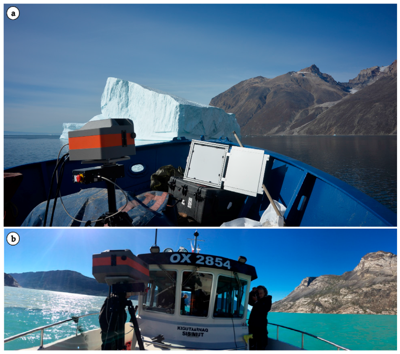
2.2.1. Instrumentation Setup

The SPECIM AisaFenix hyperspectral scanner was used to continuously scan the full wavelength range from 380 to 2500 nm using a pushbroom technology, featuring a spectral resolution of 3.5 nm and 12 nm and a sampling interval of 1.6 nm and 5 nm in VNIR and SWIR, respectively. The system was mounted on a tripod, facing the cliffs, on the foredeck of a 10 and 20 m long vessel, in Søndre Strømfjord and Karrat, respectively (Figure 2). Each datacube was constructed in the along-track direction by a uniform rotation of the sensor around the vertical axis of the tripod with a total coverage angle of about 120 degrees, and was characterized by a spatial height of 384 pixels and a spectral coverage of 624 discrete bands. To reduce the influence of the movement of the vessel, the acquisition parameters were set to a rapid scanning speed resulting in a fast frame rate of 30–40 Hz, and a short integration time of 23–28 milliseconds (ms) for VNIR and 15–20 ms for SWIR. The data were captured continuously and with sufficient overlap at a constant cruising speed of 6 knots and at a distance to the coast of 1.5 to 2.5 km, which translates into images with pixel sizes on the ground (ground sampling distance) of about 2–4 m. Each file is approximately 600 MB, and it takes approximately one minute to collect the spectral image (faster or slower scanning speed can be selected depending on the amplitude of waves and speed of the vessel).

The stereo-images were collected with a handheld camera (Nikon D800E) equipped with a 35 mm 1.4 L Zeiss Distagon T* ZE prime lens that was fixed at infinity during image acquisition. The camera was calibrated prior to field work using a test field consisting of a steel grid with around 100 marked targets, the same as that described by [57]. Images were automatically geotagged using a GPS attached to the camera allowing for an accuracy of ± 5–10 m. The images were later used to reconstruct the surface geometry. In the case of acquiring both stereo and hyperspectral images from a vessel, the positions of the camera and SPECIM AisaFenix instrument were chosen to be close to each other (a baseline of about 1.5 m) to minimize differences in viewing angles during data acquisition. To achieve a more accurate result for integration of two datasets, irrespectively of using identical or different platforms for data collection, the images are acquired with a (near-)perpendicular view to the outcrop surface.

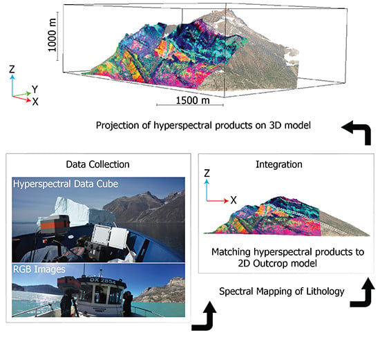
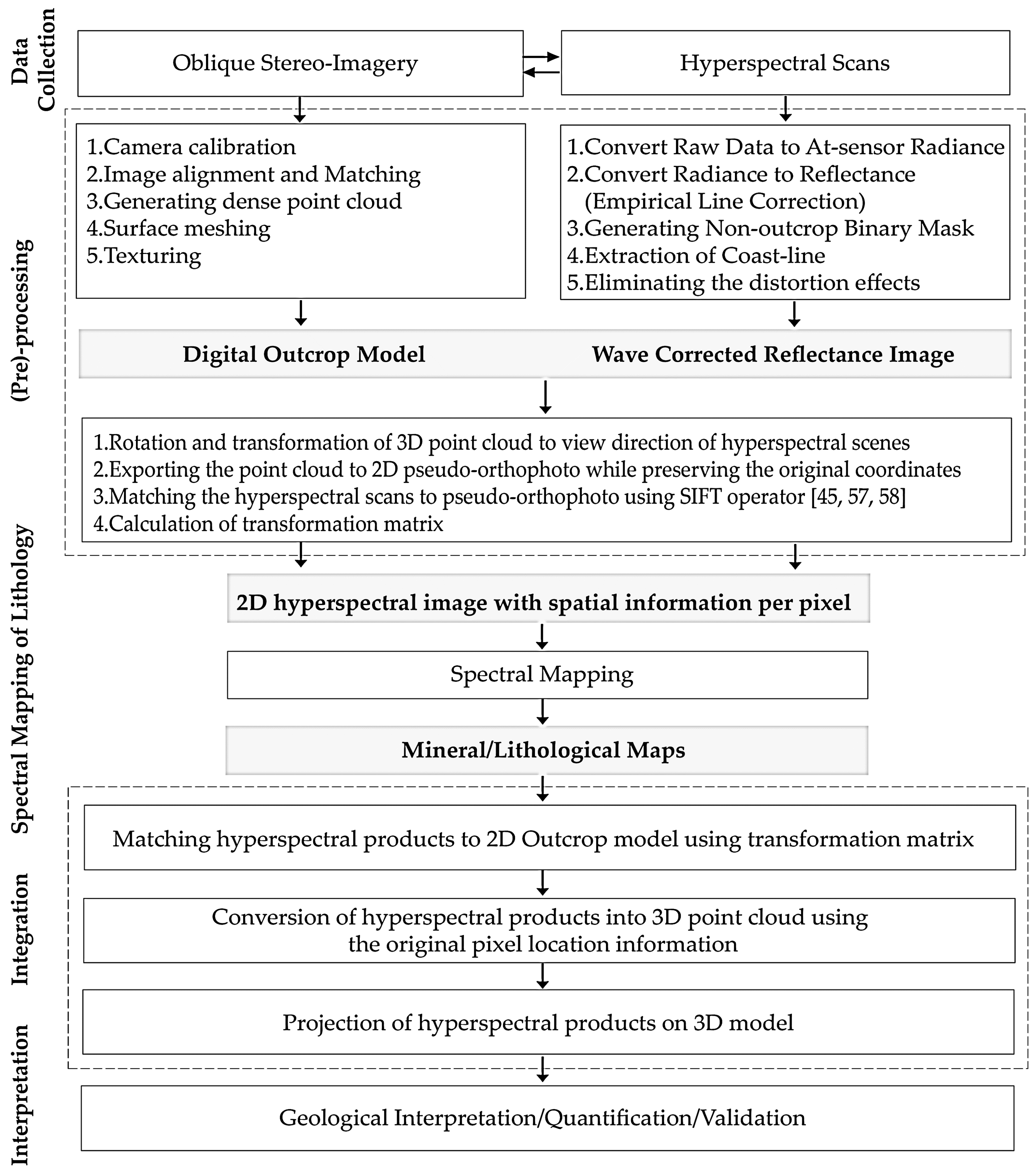
2.3. Processing Workflow

The processing workflow towards generating a 3D-surface model by fusion of high-oblique to near-horizontal stereo-images and hyperspectral horizontal scans consists of five steps (Figure 3): (1) pre-processing of hyperspectral data (i.e., retrieving surface reflectance information and eliminating the distortion effects from data); (2) reconstruction of the data acquisition geometry, referencing of the intrinsic coordinate system to available reference points (either GPS or known camera locations) and generating a dense point cloud (a digital surface model [DSM] can also be obtained from this step); (3) projection of the 3D point cloud onto a view-based pseudo-orthophoto to mimic the view direction of hyperspectral scans; (4) detection of characteristic data points (using the Scale Invariant Feature Transform (SIFT) method [58]) followed by automatic point matching using a homologous transformation (random sample consensus (RANSAC) method [59]) for matching the hyperspectral scans to the generated pseudo-orthophoto; and (5) conversion of hyperspectral products (i.e., mineral maps, etc.) into the 3D-surface model using the transformation matrix calculated in the previous step and the original pixel location information. Further details of how the workflow is accomplished are described in the following sections.

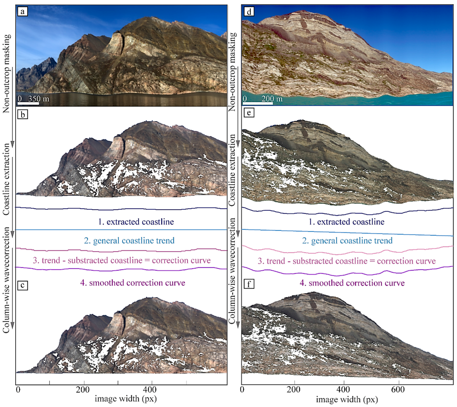
2.3.1. Pre-Processing of Hyperspectral Data

Pre-processing of hyperspectral data is an essential step for transferring the raw data into physically meaningful values and thus to implement quantitative analysis. The choice of procedure may largely depend on the spectral properties of the materials of interest. In other words, differentiating minerals with pronounced spectra differences requires less complex corrections as compared to minerals with similar spectral features. Very accurate radiometric corrections demand extensive information on the scene geometry and the atmospheric conditions at the time of acquisition. This information is usually not available during exploration in remote or inaccessible areas. As we aimed at developing a general workflow for integration of 3D-photogrammetry with vessel-based hyperspectral imaging, we focused on robust standard pre-processing steps. We balanced the needs for spectral accuracy with the costs extra steps would generate for a rapid and robust data acquisition. The aim is, therefore, not to provide the most accurate dataset but to allow the best data acquisition without penalizing the other exploration activities in a time and cost efficient manner. Detailed atmospheric/radiometric and topographic corrections are beyond the scope of this paper and will be discussed in a forthcoming paper [60].

In the first step, the raw spectral data recorded by the SPECIM AisaFenix scanner were converted into at-sensor radiances, using SPECIM’s CaligeoPRO software (version 2.2.16; Specim Spectral Imaging Ltd, Oulu, Finland) and spectral calibration files provided by the sensor manufacturer (Figure 3). The at-sensor radiance was then transferred into relative reflectance using the empirical line approach that removes the solar irradiance and the atmospheric path radiance in the image [61]. Reference spectra were provided by white panel (Spectralon, SRT-99-050) measurements with the panel positioned on the vessel during data acquisition. Using additional panels in different shades of grey could be a straightforward solution to avoid over-saturation of the white panel that was not available during the acquisition campaign. The panel is captured in every single scan to account for illumination changes between different scenes. Several factors posed challenges to the setup of hyperspectral data acquisition. First, positioning of the panel with the same distance and orientation as the outcrop was not feasible due to the inaccessibility of the observed outcrop, and the fact that the platform was in motion. As a result, several considerations needed to be taken into account to retrieve more accurate spectra as the atmosphere (water vapor) between the sensor and the outcrop influences the acquired spectra. Additionally, distances between the sensor and distant/nearby outcrop differed within one scene, which subsequently caused variations in the depths of atmospheric features. More specifically, larger distances lead to more prominent and sharper atmospheric features in the spectra. Therefore, an atmospheric reference spectrum is required to correct for these atmospheric effects. Since the positions and relations between the single atmospheric absorption features are highly dependent on the composition of the atmosphere and the concentration of the single elements, it is preferable to extract the reference spectrum from the image itself (e.g., dark objects) [62,63]. The image can then be corrected by adapting the depths of the reference atmospheric absorption spectrum, and multiplying each original pixel spectrum with the adjusted reference spectrum.

Next, water, sky and low albedo pixels were identified and masked from reflectance images using a binary mask (Figure 3). To generate the mask, representative spectra were collected and averaged from reflectance data for sky, water, vegetation, and the rock exposure (Figure 4a). Based on visual inspection, the profiles of the respective spectra indicated high contrast within the wavelength range of 2004–2453 nm and thus this range was considered appropriate to differentiate the (bright) outcrop and vegetation pixels from (dark) sky and water pixels (Figure 4a). Next, the mean reflectance value was calculated throughout the selected bands for all the pixels and a single band image (here referred to as mean reflectance image) was generated. Figure 4b displays the histogram plot of the calculated statistics for the generated image. Number of pixels and mean reflectance values are shown in y and x-axis, respectively. Water and sky spectra show lower reflectance values (mean < 0.26) within the aforementioned range as compared to vegetation and rock exposure end-members (Figure 4a,b). Based on the statistics of the mean reflectance at wavelengths 2004–2453 nm, a threshold of 0.26 (red dashed line in Figure 4b) was set to mask out pixels related to water, sky and deep topographic shading. This threshold varies slightly from acquisition to acquisition (usually most successful around 0.2) but is straightforward to identify as shown here. Masking vegetation was done by calculating the Normalized Difference Vegetation Index (NDVI) [64]. The masking threshold can be adjusted in the range between 0.35 and 0.6 for sparse to dense vegetation. Two morphological operations of erosion and dilation [65] were then applied on the generated mask to remove single isolated pixels outside the outcrop-area and fill in the gaps inside the outcrop-area.

In the next step, the distortion effects originating from the periodic movements of the vessel were eliminated from the hyperspectral scans. The coastline was extracted for this purpose, by finding the last non-zero pixel in each column of the aforementioned binary mask (from top to bottom; Figure 5b). Considering the large distance between the sensor and the coastline during data acquisition, the general coastline trend is assumed to be a flat line and was thus predicted with line-regression model (see general coastline trend in Figure 5b,e). The difference between the extracted coastline (from the binary mask, see extracted coastline in Figure 5b,e) and the reference coastline (the general coastline trend) defines the amount of shift to be applied for each column along the width of image (i.e., the correction curve) to automatically eliminate the effect of waves. Savitzky–Golay filtering was applied to smooth the calculated correction curve and remove outlier pixels remaining from the masking process [66] (see smoothed correction curve in Figure 5b,e). This is achieved in a convolution process, in which successive sub-sets (window size of 21 pixels) of adjacent data points are fitted with a second-order polynomial by the method of linear least squares. When the data points are equally spaced, an analytical solution to the least-squares equations can be found in the form of a single set of convolution coefficients. These coefficients were then applied to all data sub-sets to provide estimates of the smoothed coastline at the central point of each sub-set. Each column of the reflectance image (Figure 5a) was then shifted according to the calculated “shift values” (see smoothed correction curve in Figure 5b,e), thus correcting the image for the effect of the waves (Figure 5c).

2.3.2. Geolocation of the Stereo-Images and Point Cloud Generation

Different approaches and software packages (freeware as well as commercial) exist for the extraction of point cloud data from stereo-imagery. For the Karrat region, we used a Structure-from-Motion (SfM) approach in the Agisoft PhotoScan software for photogrammetric processing of digital images [67,68] to generate tie points (common points between the images). Depending on the quality of the camera location data available (for example, GPS data collected together with the images), it would be possible to use this information as input into the bundle adjustment solution in any SfM software and in the further processing chain. 3D Stereo Blend was used to triangulate the images using the raw-image matches from Agisoft together with a combination of pass points from monochrome aerotriangulated aerial photographs, GPS data and photogrammetrically measured sea-level points. The root mean square error on the triangulation, which is an estimate on how well the images fit the control source (aerotriangulated aerial photographs), is equal to around 3 m in x, y, and z dimensions. The resultant camera locations and orientations were then used in the next step to generate a dense point cloud using the multi-view stereo reconstruction algorithm residing within Agisoft Photoscan.

Due to the lack of aerial photographs in Søndre Strømfjord region, a dense point cloud was generated from the vessel-based stereo-images using multi-view stereo reconstruction algorithm. GPS data collected together with the images were used for absolute positioning of the point cloud. The generated point cloud has an average point density of 0.25 points·m⁻².

2.3.3. Projection of the 3D Point Cloud onto a 2D Pseudo-Orthophoto

The generated point cloud (Figure 6a) was projected onto a 2D-plane to mimic the viewing angle of the hyperspectral scenes in what we call a pseudo-orthophoto (Figure 6b). This was done by transforming, in a first step, the point cloud onto a sphere with the center point corresponding to the hyperspectral camera GPS position. Secondly, the transformed point cloud was projected cylindrically according to the camera viewing direction and rasterized into a RGB GeoTiff image (pseudo-orthophoto), preserving the original point locations as scalar values in additional image bands.

2.3.4. Matching the Hyperspectral Scans to the Pseudo-Orthophoto

To derive the spatial information per pixel for the hyperspectral imagery, these data were registered to the pseudo-orthophoto. The SIFT method was used for extracting distinctive features, invariant to image scale and rotation, that can be used to perform reliable matching between the two image sets acquired from different viewpoints and with different spatial resolutions and geometric projections [58]. This image-matching algorithm provides robust matching across a substantial range of affine distortion, for significant noise levels, complex geometric and difficult radiometric conditions and is able to handle the differences in visible appearance of features in different parts of the electromagnetic spectrum [69,70,71,72,73,74,75].

The SIFT detector operates on a single greyscale image band; therefore, the algorithm was applied on each of the three bands of the pseudo-orthophoto separately. On the other hand, hyperspectral images consist of hundreds of spectral bands and matching more than 600 hyperspectral bands with the covering pseudo-orthophoto is feasible but inefficient and time consuming. The observations suggest that the number of homologous points matched between a hyperspectral band and the covering pseudo-orthophoto varies with the wavelength, with an overall trend of fewer points to be found as a function of increasing wavelengths [42,76,77]. Furthermore, a unique point, representing a single object, is matched across multiple spectral bands if the full contiguous wavelength range (nominally 380–2500 nm) is used for the matching step. Therefore, a systematic sampling approach was used with equal intervals (i.e., 20 bands), across the entire spectral range of the SPECIM AisaFenix camera to uniformly represent the entire spectral range of the sensor, whilst limiting the information loss (maintaining the number of homologous points). Using an optimal band selection routine maximizes the number of unique points found while minimizing the input data for the SIFT algorithm [42]. Each band analyzed contributes with characteristic keypoints, which were compared with the extracted keypoints of the orthophoto using the FLANN matcher library [78] to find matching keypoints between both datasets. False matches were eliminated by fitting a fundamental matrix model with the RANSAC method [59], resulting in homologous points. Optionally, to optimize the matching conditions and shorten the processing time, the pseudo-orthophoto can be down-sampled using an area-based interpolation by a scale factor approximately equal to the ratio of the differences in pixel dimensions between the two images. As a result, the hyperspectral scans and pseudo-orthophoto will have nearly identical object sampling resolutions. It should be noted that increasing the number of matching points by changing the parameters does not necessarily increase the accuracy and can cause errors and uncertainties (wrong matches).

2.4. Spectral Mapping

Following surface reflectance calibration and elimination of distortion, the hyperspectral images can then be used for subsequent mapping and interpretation. In the present paper, three different mapping methods, namely Wavelength of Minimum [79,80], Minimum Noise Fraction (MNF) transformation [81,82] and Spectral Angle Mapper (SAM) classification [83] were applied to test the applicability of the data for mineral mapping. Non-geological material (such as vegetation) and areas strongly affected by shadows are masked (Section 2.3.1) and excluded from HIS data cubes before applying the mapping methods. The study was based on processing of the full wavelength range of 380–2500 nm for the SAM and MNF methods, whereas specific wavelength intervals in the SWIR region are selected for Minimum Wavelength Mapping. In addition to this, photogrammetric terrain data was used to extract structural information in the area, which was subsequently integrated with hyperspectral data to understand the impact of structure on spatial distribution of the minerals.

The Minimum Wavelength Mapping method is employed to explore mineral diversity and associations in the images [79]. This method is particularly useful in areas, where field validation is sparse and with imagery containing shallow spectral features. First, the deepest absorption features in a specified spectral range related to AlOH (~2160 to 2220 nm), FeOH (~2220 to 2300 nm), and MgOH (~2300 to 2360 nm) bonds are determined [84,85,86]. The absorption around (~2300 to 2350 nm) also characterizes carbonates (CO₃) [84,87]; however, based on available geological maps and our field observations, no carbonates are present in the study areas. Therefore, in this case, additional smaller absorptions around 2300 and 2350 nm are characteristic of the Fe/AlOH and Fe₂OH combination bands in phyllosilicates [88]. To highlight spectral absorptions, a continuum removal is performed over the wavelength interval. The continuum is removed for each pixel by calculation of a convex hull and its subsequent removal by division, which resulted in a normalization of the reflectance spectra to their continuum [89]. From the resulting image maps, an assessment of the dominant groups of minerals and their spatial distribution can be readily made and subtle spectral features can be analyzed.

A MNF transformation is performed on the georeferenced wave corrected hyperspectral imagery to determine the inherent dimensionality of image data and to reduce the computational requirements for subsequent processing [81,82]. For most images, the first 10–15 components of the MNF transformation show high eigenvalues (>4.5) and appear spatially coherent. Components with low and nearly equal eigenvalues were interpreted to contain mainly random noise. End-member (the spectrally most pure pixels) selection is carried out using the Pixel Purity Index (PPI) technique [90]. The PPI process exploits convex geometry concepts in the n-dimensional data space of the MNF-processed hyperspectral data. Spectra can be thought of as points in an n-dimensional scatter plot, where “n” is the number of MNF bands or dimensions. The n-D Visualizer is used to rotate the data cloud, and to find the end-members by locating and clustering the purest pixels in n-dimensional space. End-member spectra are defined by the interpretation of absorption features, and comparison with the United States Geological Survey (USGS) spectral library. This set of end-member signatures is then used in the SAM algorithm to determine locations of end-members [83]. This method is based on spectral curve analysis and is relatively insensitive to illumination and albedo effects. Since the topographic correction corrects for the relative spectral intensity between pixels without changing the spectral shape itself, and no topographic correction is conducted in this study, SAM is a well-suited technique to perform the classification. SAM compares the angle between the end-member spectrum and each pixel vector in n-dimensional space and produces a classified image based on the SAM Maximum Angle Threshold. Smaller angles represent closer (better) matches to the reference spectrum. Increasing this threshold may result in a more spatially coherent image; however, the overall pixel matches will not be as good as for the lower threshold. The output from SAM is a classified image and a set of rule images corresponding to the Spectral Angle calculated between each pixel and each end-member.

3. Results

3.1. Hyperspectral Classification

The wavelength mapping approach does not require prior definition of the end-members or any knowledge of the site conditions, as the absorption wavelength positions and depths of the major absorption features are extracted automatically. Figure 7 and Figure 8 show the resulting wavelength position maps highlighting lithological variations associated with differences in the abundance of AlOH, FeOH and MgOH bearing minerals for Karrat and Søndre Strømfjord regions, respectively. The resulting maps show images with different colors symbolizing various absorption feature wavelengths; each color shows degree of saturation at different absorption depth (Figure 7 and Figure 8). The absorption wavelength position can be correlated with minerals and their occurrences, whereas absorption depth is linked to relative abundance and grain size of certain minerals in a mixture.

Wavelength positions of deepest absorption features around 2200 nm are indicative of mica group minerals [87,91,92,93]. The amphibole group minerals have MgOH absorption features at approximately 2300 and 2380 nm and chlorite group minerals show diagnostic absorption feature around 2254 nm [91,94]. The broad red curved lines observed in the absorption feature depth maps in Søndre Strømfjord region are instrument related artifacts (Figure 8). These pixels have erroneous values between 2200 to 2300 nm. Since this wavelength range holds valuable mineralogical information and only a few lines of the image are affected, this wavelength range is not excluded from the dataset.

After compressing the main data variability of the dataset, using a MNF transformation, it is possible to assess the material spatial variability, define end-members (Figure 9) and employ an unsupervised classification (i.e., SAM). Defining and clustering the end-members is the only expert-dependent parts of the analysis. In this particular hyperspectral dataset (Figure 10b,e), the first 15 eigenvectors of the MNF transformation contain coherent information, which can be used for further processing. Visualization of the MNF bands as red-green-blue (RGB) images contributed to initial interpretation of the geology and simplified locating of the target materials for further spectral classification. Despite the low number of mineralogy related characteristic absorption features in the SWIR spectral range, a differentiation of lithological end-members is possible due to small differences in the slope, convexity and intensity of reflectance (Figure 10b,e). The shallow absorption features of surface minerals in the spectra make it difficult to separate mineralogical surface information from artifacts in the images (Figure 9). Spectra are thus normalized using the continuum removal technique to enable a detailed analysis of absorption features [89]. The main absorption related to muscovite is around 2200 nm, whereas absorption features around 2320 and 2380 nm are related to MgOH in amphiboles. The SWIR region from chlorite spectra often displays a FeOH absorption feature near 2254 nm and two MgOH features near 2320 nm and 2380 nm [94].

Hard classification, as obtained with SAM, brings the spectrum property back to a single mineral map. In reality, most pixels are mixtures; however, assignment to a hard class is based on the most pronounced absorption features representing the dominant mineral. The results from SAM approach show the variation in surface mineralogy in a variety of different colors (Figure 10c,f). The lower part of the mineral map in the Karrat region (Figure 10c) is dominated by sillimanite, sericite, pyroxene, biotite classified pixels. This part corresponds to the section that comprises Archean basement rocks. Chlorite and mica rich areas within the lower part corresponds to areas of accumulated loose material derived from the overlying Nûkavsak Formation. The overlying Nûkavsak Formation is dominated by chlorite/mica (muscovite), amphibole (actinolite), and biotite and jarosite classified pixels. This is in good correspondence with what is observed in the field and clearly reflects the generally lower metamorphic grade (greenschist to amphibolite facies) of the Nûkavsak Formation. Furthermore, the different mineralogy (pyroxene, biotite) of the overlying Archean basement nappe (Kigarsima Nappe) which has been overthrusted on top of the Nûkavsak Formation in the uppermost part of the cliff, is also detected in the mineral map. The analysis of hyperspectral imagery for Søndre Strømfjord region shows the Kangâmiut dykes intruding the intensely deformed Archean gneisses (Figure 10f). The foliation is clearly identifiable and several ductile and brittle structures can be observed in the dykes. Amphiboles represent the dominant minerals of these dykes, whereas mica as well as pyroxene are present at secondary abundances.

3.2. Integration

3.2.1. Matching Hyperspectral Products to the 2D Outcrop Model Using Transformation Matrix

Different methods can be applied to determine the transformation parameters for matching the hyperspectral data to the pseudo-orthophoto depending on the complexity of the scene. In this study, the matching points derived from the SIFT method are used as control points to establish correspondence between the hyperspectral imagery and the 2D pseudo-orthophoto using GDALWarp-polynomial fitting function [95]. Once the correspondence between the hyperspectral scans and the pseudo-orthophoto is found (pixel coordinates of homologous points), the transformation matrix is used to project the individual hyperspectral products on the 2D pseudo-orthophoto (Figure 10). The georeferencing and its success highly depends upon the accuracy of the viewing angle used for the resulting pseudo-orthophoto. Exploiting inaccurate viewing angle would complicate the matching process by finding no, less or wrong points and thus would increase the required processing time. Additionally, forced matching of the two image-sets induces distortions in the resulting georeferenced AisaFENIX hyperspectral scan by strong interpolation of pixels and therefore will have possible impacts on the final mapping results.

3.2.2. Transformation of Hyperspectral Products into a 3D Model

For each pixel in the hyperspectral products, 3D object space coordinates are derived by merging the original orthophoto pixel locations preserved from previous steps to the new hyperspectral color information (Figure 11). The 3D viewing allows the visualization and interpretation of hyperspectral image products in conjunction with the 3D outcrop models.

3.3. Evaluation

No ground truth is available for the direct validation of the dataset acquired. To allow for a quantitative evaluation of the accuracy of the method, the coordinates of 10 control points (CPs), which were manually extracted from the 2D pseudo-orthophoto, were compared to the ones from the warped hyperspectral images by measuring distances in pixels between these related points. Experiments show that the RMSE (Root-Mean-Square Error) in x and y directions is 6.7 and 8.4 pixels for Karrat and 3.9 and 4.5 pixels for Søndre Strømfjord, respectively (

Table 1. Quantitative evaluation of the registration accuracy using handpicked control points from the pseudo-orthophotos. Coordinates for the CPs are assessed against the corresponding coordinates in reconstructed hyperspectral data along X and Y axes.

Study	ID	X-Ortho (Pixels)	Y-Ortho	X-Fenix	Y-Fenix (Pixels)	Diff-X (Pixels)	Diff-Y (Pixels)
Karrat	CP 1	193.8593	193.8593	190.6042	517.9694	3.2552	2.9267
	CP 2	219.3461	219.3461	220.2049	300.3276	−0.8589	−11.1290
	CP 3	350.2552	350.2552	357.8391	481.0251	−7.5839	0.4825
	CP 4	211.2367	211.2367	201.6286	802.7344	9.6081	0.8329
	CP 5	21.24463	21.24463	35.28549	786.6907	−14.0409	12.2430
	CP 6	232.0895	232.0895	235.4142	214.2756	−3.3247	−13.1219
	CP 7	381.5344	381.5344	380.6374	864.7964	0.8970	−14.8896
	CP 8	188.0669	188.0669	183.0522	954.3008	5.0147	3.3454
	CP 9	98.86334	98.86334	94.81434	400.3867	4.0490	1.1852
	CP 10	122.0331	122.0331	128.1674	746.1608	−6.1343	−2.8350
						RSME-X	RSME-Y (pixels)
						6.7	8.4
Søndre Strømfjord	CP 1	140.3506	922.3118	134.8122	915.8555	5.5383	6.4563
	CP 2	105.2719	880.0375	106.2451	877.352	−0.9732	2.6855
	CP 3	29.7179	713.6388	30.48011	719.6117	−0.7622	−5.9730
	CP 4	265.3745	854.8528	266.0554	855.8231	−0.6810	−0.9703
	CP 5	212.3068	642.582	215.5454	650.471	−3.2387	−7.8890
	CP 6	343.6269	1202.941	350.5148	1204.425	−6.8879	−1.4839
	CP 7	216.8041	1007.76	217.6155	1009.423	−0.8115	−1.6634
	CP 8	161.9374	460.8926	162.9654	453.8132	−1.0279	7.0793
	CP 9	36.01406	415.9199	28.82405	415.7237	7.1900	0.1962
	CP 10	265.3745	1056.33	268.1255	1057.449	−2.7510	−1.1189
						RSME-X	RSME-Y (pixels)
						3.9	4.5

).

4. Discussion

Usually, the complex geology of Greenland is mapped using visual panoramas accessible either from helicopter or from boat with only few incursions of field mapping on-shore. Photogeology based on RGB acquisitions completes the limited in situ observations. Blind headwall and sidewall faults are located and extrapolated to depth using an iterative technique involving geological map interpretation and construction of cross-sections validated by restoration. Terrestrial imaging spectrometry for mapping of near vertical geological outcrops has been the topic of many studies in recent years [35,36,37,38]. This approach has been applied in the Arctic by scanning the vertical cliffs from an opposing location such as a neighboring mountain [48,60]. However, such approach is not always feasible where data are to be acquired on a routine operational basis to provide information on mineralogy as part of large-scale mapping operations. In addition, such scanning might not be possible when dealing with steep coastal cliff sections where terrain accessibility hinders instrumentation setup.

We introduce here a novel and flexible approach for mapping near-vertical cliff sections along fjords, coastlines and valleys in remote regions, which are difficult to map by means of classic geological field campaigns or space-airborne remote sensing surveys. The results stress the use of detailed spectral information from HSI and the geometric information from high-resolution photogrammetry data as valuable support for meaningful outcrop analysis. Using the association of 3D photogrammetry with spectral data has two main contributions to the existing tools available to the cartographers. First, as depicted in Figure 10c,f, the hyperspectral data allow one to determine mineral associations directly (e.g., minerals such as jarosite or chlorite) or indirectly (using proxies such as AlOH). Mapping is therefore not only based on stratigraphy but on mineralogical-petrological data. The known formations can easily be discriminated based on known geological structures such as the presence of lenses or boudins with characteristic mineralogies. This enables geologists to distinguish the spatial distribution of different rock types and minerals, in a non-contact manner, which is beneficial for exploration in the arctic environment. Secondly, the point cloud allows the determination of the real orientation of structures or lithologies. The knowledge of the spatial coordinates of points belonging to planar features, such as bedding or faults, allows the calculation of the planes they belong to. The resulting point cloud can be further analyzed with calculations of outcrop parameters such as surface roughness and curvature, or with more sophisticated calculations used in semi-automatic tracing of discontinuities, such as joints, fractures or beddings. A precise understanding of both geometry and nature of the geology is very relevant for mineral exploration. In other words, the HSI results can be joined with topographical and structural features and a combined 3D outcrop model can be created to visualize the mapping results, which is an important addition to the way 3D mapping is undertaken in the arctic. It has been postulated that the MVT Pb–Zn deposits at Maarmorilik (Black Angel Mine in central west Greenland) may have been emplaced during fluid migration in response to the Nunaarsussuaq thrust system advancing from the SE [48]. Better information on fault geometries and hydrothermal alterations are thus fundamental for the localization of potential ore deposits. This information is provided by the combination of HSI and SfM photogrammetry.

In the present study, scanning of the entire outcrop was achieved within one working day. The automated workflow enables an easy processing of scenes of a large campaign and a much faster provision of such data compared to manual approaches. Batch processing on multiple spectral data is conducted for most of the preprocessing steps, and takes a few minutes for each spectral scene. With respect to computational time, we observed that the most time-consuming part is generating the correct pseudo-orthophotos required for accurate matching of the two datasets. This is comparable in time to the setup of the stereo-images and subsequent extraction of terrain models. The matching procedure also takes one to two days depending on the actual outcrop, the size of the point cloud, and the accuracy of the camera position and orientation. The processing time can be greatly reduced if these parameters are set correctly. This study confirms the ease with which this method can be applied, but also shows that the various sensors used and the environmental effects encountered can make the calibration and analysis of these data types, a challenge. As a result, several theoretical assumptions and practical considerations should be taken into account before applying this approach:

• Accurate setup of white panel within the same distance and orientation as the outcrop, essential for a realistic conversion to reflectance values, is not possible due to the inaccessibility of the observed outcrop and the fact that the platform is in motion. Consequently, the atmosphere between the vessel and vertical cliffs affects the surface reflectance spectra. Further spectral processing is needed for eliminating these effects to ensure accurate and reliable image spectra, which is crucial for the discrimination of geological targets and detailed spectral mapping applications.
• Collecting ground reflectance measurements from homogenous targets can be a solution for calculating the calibration coefficients for each band and removing the effects of atmospheric scattering and absorption to retrieve reliable data. However, when collecting reflectance spectra of the targets on the ground, sufficient measurements should be made to adequately represent any heterogeneity in the target, which due to the nature of near-vertical cliff sections is not always an option. In addition, if there is to be any time-lag between the collection of ground and vessel based data, then the spectral stability of the surface over time should be considered. Thus, it is not a feasible approach, if data are to be acquired on a large spatial scale and within a short amount of time, typical for geological surveys in the Arctic. This can alternatively be achieved by selecting an atmospheric reference spectrum from the image and correcting the image spectra based on the actual depth of atmospheric features. This approach requires additional development and could be a scope for follow-up research.
• An additional sensor-based challenge stems from the differences in the acquisition technology of frame-based RGB cameras and hyperspectral push-broom scanners rotating on a tripod. The resulting differences in viewing angle and perspective distortion can make the integration of datasets difficult. As CloudCompare (version 2.9) only supports rasterizing using orthographic view to project the point cloud onto a 2D plane, a python script was developed as part of this study to generate the perspective view for reconstructing the accurate viewing angle.
• From the mapping perspective, rocks of different chemical or mineral composition are sometimes characterized by only subtle differences in reflectance spectra [84,96,97]. However, in the context of steeply dipping cliff faces, variability in incident light also occurs causing spectral noise, which may exceed the effect of the intrinsic composition of the rocks. In such cases, it is not possible to uniquely separate and map rock units on vertical cliffs. Thus, it is essential to correct for these effects to retrieve reliable data. Moreover, surrounding topography can have a high influence on the local illumination within an image and can influence the measured at-sensor radiance by casting shadows, blocking diffuse sky irradiance or adding additional ground reflections [35]. The radiance of the same material varies, if it is located on a slope oriented toward or away from the sunlight incidence and optimal results are therefore achieved, when the view of the sensor is perpendicular to the slope of the outcrop.
• Shadows and change of scale could lead to misidentification of elevation points within the stereo model. In the present study, the experiments were performed in cloudy weather and the outcrop had a uniform steep slope without major changes in scale. The experiments as such were therefore conducted under optimal conditions.
• Considering the specification of the hyperspectral camera used here and assuming a range of 1.5 to 2.5 km, the ground pixel size would be approximately 2–4 m. This will pose a problem for the matching of datasets if the photogrammetric point cloud is too high in spatial resolution (i.e., cm pixel size in this study). As a solution, the point cloud can be downscaled (resampled) for finding transformation matrix and later be used with the original scale to perform geological mapping.
• Overall, the advantages of the method clearly outweigh the limitations, if those are considered during data processing and taken into account for the interpretation of the results.

Although the experiment clearly shows the potential of using horizontal hyperspectral scanning and stereo-images for DOM generation for geological purposes, further testing in different settings, scales and conditions would be beneficial to determine how the hyperspectral sensor performs under different conditions. Generating detailed 3D outcrop models using platforms in motion and horizontal scanning needs further testing at longer ranges and for different conditions. Similar studies could be undertaken elsewhere and could be used to evaluate how well the conceptual understanding of an area fits with the “real” three-dimensional structure. Data made available within this study could form the backdrop of such detailed models. Furthermore, the method is not specifically designed for AisaFenix hyperspectral data, and can easily be adapted to any available hyperspectral sensor. Considering the fast development in various sensors (higher spectral and spatial resolution, better performance, smaller sizes and lower weight) this method can be deployed from other platforms such as helicopters, small airplanes or drones. Therefore, central to the presented workflow is the flexibility and mobility of the method to provide information on mineralogy as part of large-scale mapping operations (i.e., areas of hundreds or thousands of square kilometers). This makes the method highly efficient in logistically challenging field areas like Greenland. Additionally, the proposed workflow is not limited to lithological mineral mapping in the Arctic as the same concept can be used for other applications. An interesting aspect, e.g., would be to integrate and compare the models with geophysical properties or to constrain geophysical inversion models along the surface.

5. Conclusions

To the authors’ best knowledge, this is the first time a vessel is used for acquisition of spectral data from vertical cliffs. Deployment of a platform in motion as opposed to terrestrial scanning has the advantage that it is highly flexible and well suited for difficult and remote terrains, where a logistic platform would provide a cheaper and time efficient solution as compared to the use of terrestrial scanning. This simplifies the expansion of mapping in remote places (e.g., in Greenland), where a large proportion of the area is still under-explored and the lack of infrastructure reduces the capabilities to economically explore and locate mineral resources using traditional techniques. The proposed automatic approach for combining spectral and point cloud data is a timesaving alternative to manual approaches and has high potential for field geologists, who wish to establish accurate outcrop models that can be brought to life and visualized in 3D surface models. These models can be freely rotated in three dimensions and are well suited for visualization as well as for quantitative purposes in geological mapping or in the preparation for field operations. The algorithms implemented work reliably even for complex geometries and with high accuracy. Slightly distorted data, such as images over a low-relief landscape, can be treated quickly using homographic or polynomial transformations and even the data with high local distortions caused by the underlying topography can be processed. The key findings of this study are as following:

• The SIFT image-matching algorithm performs reliable matching between the two image sets acquired from different viewpoints and with different spatial resolution and geometric projections (i.e., spectral data with aerial high-oblique stereo-images collected from a helicopter or near-horizontal stereo-images collected from a vessel using hand-held digital cameras).
• Larger vessels provide a more stable platform for data acquisition (i.e., less pronounced pitch and heave result in less distortion in the HSI data). Nevertheless, the presented method can cope with the data captured from both small and large vessels.
• The spectral mapping of hyperspectral imagery of vertical cliffs is not straightforward because of: (a) the relatively shallow absorption features of surface minerals in the spectra; (b) the instrument artifacts present in the data; and (c) the lack of ground samples of surface materials.
• Despite the low number of mineralogy related characteristic absorption features in the SWIR spectral range, a differentiation of lithological end-members is possible due to small differences in the slope, convexity and intensity of the reflectance spectra.
• Three methods are deployed to make an assessment of the information content of the hyperspectral images and the group of minerals present in the images: Mapping the wavelength position of the deepest absorption features between 2100 and 2400 nm provides a useful method for exploratory analysis of the surface mineralogy of vertical cliffs. By using a MNF transformation, it is possible to assess the material spatial variability, define end-members and employ a supervised classification. The SAM method provides information on the diversity and composition of minerals and their occurrences on the surface. However, assigning pixels to mineral classes could cause a loss of information.
• The empirical line correction method assumes that there are no differences in illumination across the image; therefore, changes in radiance due to cloud shadowing or topography are not corrected. In addition to sensor and platform/specific geometric distortion corrections, a subsequent topographic correction is highly recommended for sites with high relief or sub/optimal illumination conditions during data acquisition. Using continuum removal in a wavelength mapping technique reduces shadow effects and differences in scene illumination, which enables the production of seamless map products. However, by doing so, the spectral albedo, which links to the brightness of an object, is discarded. More importantly, the overall reflectance is also a key to handle mapping of spectrally featureless minerals.
• The method also assumes that the effect of the atmosphere is uniform across the image, but it has been observed that atmospheric constituents, especially water vapor, can vary greatly over short distances.
• The method assumes that the earth’s surface consists of Lambertian reflectors, when in fact the surfaces possess bi-directional reflectance properties [98,99], which will cause viewing geometry to be an important control over the accuracy of the prediction equations. Non-Lambertian reflectance is largely due to the presence of shadows caused by surface micro-relief. Further development of the methodology will require consideration of the bi-directional reflectance properties of the targets, and measurement of the spatial variability of the atmospheric path radiance throughout the image.
• The choice of the reference spectrum for removing the effect of atmosphere between the vessel and the outcrop has a high influence on the quality of the spectral data and needs to be investigated carefully, as it can otherwise create non-atmospheric absorption features. The reference spectra should be selected: (a) from homogeneous extensive bare areas (at least several times the size of the sensor ground instantaneous field-of-view) that are preferably located vertically; (b) devoid of vegetation or other temporally variant features; and (c) ideally spectrally featureless.
• Finally, we experienced that more accurate results can be achieved, if a perpendicular view to the surface of outcrop is set for data acquisition and a view-based projection of 3D point cloud onto 2D pseudo-orthophotos is used to project the individual hyperspectral products on the 2D pseudo-orthophoto. Exploiting inaccurate viewing angle would complicate the matching process of the two image-sets, thereby inducing distortions in the resulting georeferenced hyperspectral scan, and therefore will have possible impacts on the final mapping results.

References

1. Sørensen, E.V. Implementation of Digital Multi-Model Photogrammetry for Building of 3D-Models and Interpretation of the Geological and Tectonic Evolution of the Nuussuaq Basin. Ph.D. Thesis, University of Copenhagen, Copenhagen, Denmark, 2011. [Google Scholar]
2. Svennevig, K.; Guarnieri, P.; Stemmerik, L. From oblique photogrammetry to a 3d model–structural modeling of Kilen, eastern north Greenland. Comput. Geosci. 2015, 83, 120–126. [Google Scholar] [CrossRef]
3. Sørensen, E.V.; Bjerager, M.; Citterio, M. Digital models based on images taken with handheld cameras–examples on land, from the sea and on ice. Geol. Surv. Den. Greenl. Bull. 2015, 73–76. [Google Scholar]
4. Sørensen, E.V.; Pedersen, A.K.; García-Sellés, D.; Strunck, M.N. Point clouds from oblique stereo-imagery: Two outcrop case studies across scales and accessibility. Eur. J. Remote Sens. 2015, 48, 593–614. [Google Scholar] [CrossRef]
5. Vosgerau, H.; Guarnieri, P.; Weibel, R.; Larsen, M.; Dennehy, C.; Sørensen, E.V.; Knudsen, C. Study of a palaeogene intrabasaltic sedimentary unit in southern east Greenland: From 3-d photogeology to micropetrography. Geol. Surv. Den. Greenl. Bull. 2010, 20, 75–78. [Google Scholar]
6. Óskarsson, B.V.; Andersen, C.B.; Riishuus, M.S.; Sørensen, E.V.; Tegner, C. The mode of emplacement of neogene flood basalts in eastern Iceland: The plagioclase ultraphyric basalts in the grænavatn group. J. Volcanol. Geother. Res. 2017, 332, 26–50. [Google Scholar] [CrossRef]
7. Vosgerau, H.; Passey, S.R.; Svennevig, K.; Strunck, M.N.; Jolley, D.W. Reservoir architectures of interlava systems: A 3d photogrammetrical study of eocene cliff sections, Faroe Islands. Geol. Soc. Lond. Spec. Publ. 2016, 436, 55–73. [Google Scholar] [CrossRef]
8. Buckley, S.; Vallet, J.; Braathen, A.; Wheeler, W. Oblique helicopter-based laser scanning for digital terrain modelling and visualisation of geological outcrops. In Proceedings of the International Archives of Photogrammetry, Remote Sensing and Spatial Information Sciences, Beijing, China, 3–11 July 2008; Volume 37, pp. 493–498. [Google Scholar]
9. Vallet, J.; Skaloud, J. Development and experiences with a fully-digital handheld mapping system operated from a helicopter. In Proceedings of the XX ISPRS Congress, Istanbul, Turkey, 12–23 July 2004; Volume XXXV. [Google Scholar]
10. Pedersen, A.K.; Larsen, L.M.; Pedersen, G.K.; Dueholm, K.S. Five slices through the Nuussuaq basin, west Greenland. Geol. Surv. Den. Greenl. Bull. 2006, 10, 53–56. [Google Scholar]
11. Svennevig, K.; Guarnieri, P. From 3d mapping to 3d modelling: A case study from the skaergaard intrusion, southern east Greenland. Geol. Surv. Den. Greenl. Bull. 2012, 26, 57–60. [Google Scholar]
12. Pedersen, A.; Watt, M.; Watt, W.; Larsen, L. Structure and stratigraphy of the early tertiary basalts of the Blosseville Kyst, east Greenland. J. Geol. Soc. 1997, 154, 565–570. [Google Scholar] [CrossRef]
13. Bellian, J.A.; Kerans, C.; Jennette, D.C. Digital outcrop models: Applications of terrestrial scanning lidar technology in stratigraphic modeling. J. Sediment. Res. 2005, 75, 166–176. [Google Scholar] [CrossRef]
14. Buckley, S.J.; Howell, J.A.; Enge, H.D.; Kurz, T.H. Terrestrial laser scanning in geology: Data acquisition, processing and accuracy considerations. J. Geol. Soc. 2008, 165, 625–638. [Google Scholar] [CrossRef]
15. Buckley, S.J.; Enge, H.D.; Carlsson, C.; Howell, J.A. Terrestrial laser scanning for use in virtual outcrop geology. Photogramm. Rec. 2010, 25, 225–239. [Google Scholar] [CrossRef]
16. Buckley, S.J.; Howell, J.A.; Enge, H.D.; Leren, B.L.S.; Kurz, T.H. Integration of terrestrial laser scanning, digital photogrammetry and geostatistical methods for high-resolution modelling of geological outcrops. Remote Sens. Spat. Inf. Sci. 2006, 36, 6. [Google Scholar]
17. Enge, H.D.; Buckley, S.J.; Rotevatn, A.; Howell, J.A. From outcrop to reservoir simulation model: Workflow and procedures. Geosphere 2007, 3, 469–490. [Google Scholar] [CrossRef]
18. Crowley, J.K. Visible and near-infrared spectra of carbonate rocks: Reflectance variations related to petrographic texture and impurities. J. Geophys. Res. Solid Earth 1986, 91, 5001–5012. [Google Scholar] [CrossRef]
19. Gaffey, S.J. Spectral reflectance of carbonate minerals in the visible and near infrared (O.35-2.55 microns); calcite, aragonite, and dolomite. Am. Mineral. 1986, 71, 151–162. [Google Scholar]
20. Hunt, G.R.; Salisbury, J.W. Visible and near infrared spectra of minerals and rocks. II. Carbonates. Mod. Geol. 1971, 2, 23–30. [Google Scholar]
21. Van der Meer, F. Spectral reflectance of carbonate mineral mixtures and bidirectional reflectance theory: Quantitative analysis techniques for application in remote sensing. Remote Sens. Rev. 1995, 13, 67–94. [Google Scholar] [CrossRef]
22. Van der Meer, F. Spectral mixture modelling and spectral stratigraphy in carbonate lithofacies mapping. ISPRS J. Photogramm. Remote Sens. 1996, 51, 150–162. [Google Scholar] [CrossRef]
23. Van der Meer, F.D.; De Jong, S.M. Imaging Spectrometry: Basic Principles and Prospective Applications; Springer Science & Business Media: Berlin/Heidelberg, Germany, 2011; Volume 4. [Google Scholar]
24. Solomon, J.; Rock, B. Imaging spectrometry for earth remote sensing. Science 1985, 228, 1147–1152. [Google Scholar]
25. Bellian, J.A.; Beck, R.; Kerans, C. Analysis of hyperspectral and lidar data: Remote optical mineralogy and fracture identification. Geosphere 2007, 3, 491–500. [Google Scholar] [CrossRef]
26. Bowen, B.B.; Martini, B.A.; Chan, M.A.; Parry, W.T. Reflectance spectroscopic mapping of diagenetic heterogeneities and fluid-flow pathways in the Jurassic Navajo sandstone. AAPG Bull. 2007, 91, 173–190. [Google Scholar] [CrossRef]
27. Harris, J.R.; Rogge, D.; Hitchcock, R.; Ijewliw, O.; Wright, D. Mapping lithology in canada’s arctic: Application of hyperspectral data using the minimum noise fraction transformation and matched filtering. Can. J. Earth Sci. 2005, 42, 2173–2193. [Google Scholar] [CrossRef]
28. Windeler, D.; Lyon, R. Discrimination dolomitization of marble in the Ludwig skarn near yerington, Nevada using high-resolution airborne infrared imagery. Photogramm. Eng. Remote Sens. 1991, 57, 1171–1177. [Google Scholar]
29. Bedini, E. Mapping lithology of the sarfartoq carbonatite complex, southern west Greenland, using hymap imaging spectrometer data. Remote Sens. Environ. 2009, 113, 1208–1219. [Google Scholar] [CrossRef]
30. Bedini, E. Mineral mapping in the Kap Simpson complex, central east Greenland, using hymap and aster remote sensing data. Adv. Space Res. 2011, 47, 60–73. [Google Scholar] [CrossRef]
31. Bedini, E. Mapping alteration minerals at malmbjerg molybdenum deposit, central east Greenland, by kohonen self-organizing maps and matched filter analysis of hymap data. Int. J. Remote Sens. 2012, 33, 939–961. [Google Scholar] [CrossRef]
32. Tukiainen, T.; Thomassen, B. Application of airborne hyperspectral data to mineral exploration in north-east Greenland. Geol. Surv. Den. Greenl. Bull. 2010, 20, 71–74. [Google Scholar]
33. Bedini, E.; Tukiainen, T. Using spectral mixture analysis of hyperspectral remote sensing data to map lithology of the sarfartoq carbonatite complex, southern west Greenland. Geol. Surv. Den. Greenl. Bull 2009, 17, 69–72. [Google Scholar]
34. Salehi, S.; Jakob, S.; Gloaguen, R.; Fensholt, R. Multiscale hyperspectral analysis of lithologies in presence of abundant lichens and mapping of ultramafic rocks in western Greenland (innarsuaq). In Proceedings of the 10th EARSeL SIG Imaging Spectroscopy Workshop, Zurich, Switzerland, 19–21 April 2017. [Google Scholar]
35. Kurz, T.H.; Buckley, S.J.; Howell, J.A. Close-range hyperspectral imaging for geological field studies: Workflow and methods. Int. J. Remote Sens. 2013, 34, 1798–1822. [Google Scholar] [CrossRef]
36. Kurz, T.H.; Dewit, J.; Buckley, S.J.; Thurmond, J.B.; Hunt, D.W.; Swennen, R. Hyperspectral image analysis of different carbonate lithologies (limestone, karst and hydrothermal dolomites): The pozalagua quarry case study (Cantabria, north-west Spain). Sedimentology 2012, 59, 623–645. [Google Scholar] [CrossRef]
37. Murphy, R.J.; Monteiro, S.T. Mapping the distribution of ferric iron minerals on a vertical mine face using derivative analysis of hyperspectral imagery (430–970 nm). ISPRS J. Photogramm. Remote Sens. 2013, 75, 29–39. [Google Scholar] [CrossRef]
38. Murphy, R.J.; Monteiro, S.T.; Schneider, S. Evaluating classification techniques for mapping vertical geology using field-based hyperspectral sensors. IEEE Trans. Geosci. Remote Sens. 2012, 50, 3066–3080. [Google Scholar] [CrossRef]
39. Buckley, S.J.; Kurz, T.H.; Howell, J.A.; Schneider, D. Terrestrial lidar and hyperspectral data fusion products for geological outcrop analysis. Comput. Geosci. 2013, 54, 249–258. [Google Scholar] [CrossRef]
40. Zhang, Q.; Pless, R. Extrinsic calibration of a camera and laser range finder (improves camera calibration). In Proceedings of the IEEE/RSJ International Conference on Intelligent Robots and Systems (IROS 2004), Sendai, Japan, 28 September–2 October 2004; pp. 2301–2306. [Google Scholar]
41. Kurz, T.H.; Buckley, S.J.; Howell, J.A.; Schneider, D. Integration of panoramic hyperspectral imaging with terrestrial lidar data. Photogramm. Rec. 2011, 26, 212–228. [Google Scholar] [CrossRef]
42. Sima, A.A.; Buckley, S.J.; Kurz, T.H.; Schneider, D. Semi-automated registration of close-range hyperspectral scans using oriented digital camera imagery and a 3d model. Photogramm. Rec. 2014, 29, 10–29. [Google Scholar] [CrossRef]
43. Monteiro, S.T.; Nieto, J.; Murphy, R.; Ramakrishnan, R.; Taylor, Z. Combining strong features for registration of hyperspectral and lidar data from field-based platforms. In Proceedings of the 2013 IEEE International Conference on Geoscience and Remote Sensing Symposium (IGARSS), Melbourne, Australia, 21–26 July 2013; pp. 1210–1213. [Google Scholar]
44. Kurz, T.; Buckley, S.; Howell, J.; Schneider, D. Geological outcrop modelling and interpretation using ground based hyperspectral and laser scanning data fusion. In Proceedings of the International archives of Photogrammetry, Remote Sensing and Spatial Information Sciences, Beijing, China, 3–11 July 2008; Volume 37, pp. 1229–1234. [Google Scholar]
45. Jakob, S.; Zimmermann, R.; Gloaguen, R. The need for accurate geometric and radiometric corrections of drone-borne hyperspectral data for mineral exploration: Mephysto—A toolbox for pre-processing drone-borne hyperspectral data. Remote Sens. 2017, 9, 88. [Google Scholar] [CrossRef]
46. Grocott, J.; McCaffrey, K.J. Basin evolution and destruction in an early Proterozoic continental margin: The rinkian fold–thrust belt of central west Greenland. J. Geol. Soc. 2017, 174, 453–467. [Google Scholar] [CrossRef]
47. Henderson, G.; Pulvertaft, T. Geological Map of Greenland, 1: 100000, Mârmorilik 71 v. 2 syd, Nûgâtsiaq 71 v. 2 Nord, Pangnertôq 72 v. 2 syd; Descriptive Text; Grønlands Geologiske Undersøgelse: Copenhagen, Denmark, 1987; Volume 8. [Google Scholar]
48. Rosa, D.; Dewolfe, M.; Guarnieri, P.; Kolb, J.; LaFlamme, C.; Partin, C.; Salehi, S.; Vest Sørensen, E.; Thaarup, S.; Thrane, K.; et al. Architecture and Mineral Potential of the Paleoproterozoic Karrat Group, West Greenland. Results of the 2016 Season, 5; Geological Survey of Denmark and Greenland: Copenhagen, Denmark, 2017; p. 114. Available online: https://data.geus.dk/greenlanddb/webresources/dodex-report-file/released-report/32501 (accessed on 9 September 2017).
49. Cadman, A.; Tarney, J.; Bridgwater, D.; Mengel, F.; Whitehouse, M.; Windley, B. The petrogenesis of the kangâmiut dyke swarm, W. Greenland. Precambrian Res. 2001, 105, 183–203. [Google Scholar] [CrossRef]
50. Ramberg, H. Titanic iron ore formed by dissociation of silicates in granulite facies [Greenland]. Econ. Geol. 1948, 43, 553–570. [Google Scholar] [CrossRef]
51. Bridgwater, D.; Mengel, F.; Fryer, B.; Wagner, P.; Hansen, S.C. Early Proterozoic mafic dykes in the north atlantic and baltic cratons: Field setting and chemistry of distinctive dyke swarms. Geol. Soc. Lond. Spec. Publ. 1995, 95, 193–210. [Google Scholar] [CrossRef]
52. Ramberg, H. On the Petrogenesis of the Gneiss Complexes between Sukkertoppen and Christianshaab, West Greenland. Available online: http://2dgf.dk/xpdf/bull-1948-11-3-312-327.pdf (accessed on 9 September 2017).
53. Escher, A.; Escher, J.; Watterson, J. The reorientation of the kangâmiut dike swarm, west Greenland. Can. J. Earth Sci. 1975, 12, 158–173. [Google Scholar] [CrossRef]
54. Connelly, J.N.; Mengel, F.C. Evolution of Archean components in the paleoproterozoic Nagssugtoqidian orogen, west Greenland. Geol. Soc. Am. Bull. 2000, 112, 747–763. [Google Scholar] [CrossRef]
55. Engström, J.; Klint, K.E.S. Continental collision structures and post-orogenic geological history of the kangerlussuaq area in the southern part of the nagssugtoqidian orogen, central west Greenland. Geosciences 2014, 4, 316–334. [Google Scholar] [CrossRef]
56. Rosa, D.; Guarnieri, P.; Hollis, J.; Kolb, J.; Partin, C.; Petersen, J.; Vest Sørensen, E.; Thomassen, B.; Thomsen, L.; Thrane, K. Architecture and Mineral Potential of the Paleoproterozoic Karrat Group, West Greenland; Results of the 2015 Season; Geological Survey of Denmark and Greenland: Copenhagen, Denmark, 2016; p. 98. [Google Scholar]
57. Dueholm, K.S. Geologic photogrammetry using standard small-frame cameras. Grønl. Geol. Unders. 1992, 156, 7–17. [Google Scholar]
58. Lowe, D.G. Object recognition from local scale-invariant features. In Proceedings of the seventh IEEE International Conference on Computer Vision, Kerkyra, Greece, 20–27 September 1999; pp. 1150–1157. [Google Scholar]
59. Fischler, M.A.; Bolles, R.C. Random sample consensus: A paradigm for model fitting with applications to image analysis and automated cartography. Commun. ACM 1981, 24, 381–395. [Google Scholar] [CrossRef]
60. Lorenz, S.; Salehi, S.; Kirsch, M.; Zimmermann, R.; Unger, G.; Gloaguen, R. Radiometric correction and 3d integration of long-range ground-based hyperspectral imagery for mineral exploration of vertical outcrops. submitted.
61. Smith, G.M.; Milton, E.J. The use of the empirical line method to calibrate remotely sensed data to reflectance. Int. J. Remote Sens. 1999, 20, 2653–2662. [Google Scholar] [CrossRef]
62. Chavez, P.S. Image-based atmospheric corrections-revisited and improved. Photogramm. Eng. Remote Sens. 1996, 62, 1025–1035. [Google Scholar]
63. Vicente-Serrano, S.M.; Pérez-Cabello, F.; Lasanta, T. Assessment of radiometric correction techniques in analyzing vegetation variability and change using time series of landsat images. Remote Sens. Environ. 2008, 112, 3916–3934. [Google Scholar] [CrossRef]
64. Wessman, C.A.; Bateson, C.; Curtiss, B.; Benning, T.L. A comparison of spectral mixture analysis an ndvi for ascertaining ecological variables. In Proceedings of the 4th Annual JPL Airborne Geoscience Workshop, Washington, DC, USA, 25–29 October 1993. [Google Scholar]
65. Haralick, R.M.; Sternberg, S.R.; Zhuang, X. Image analysis using mathematical morphology. IEEE Trans. Pattern Anal. Mach. Intell. 1987, 532–550. [Google Scholar] [CrossRef]
66. Savitzky, A.; Golay, M.J. Smoothing and differentiation of data by simplified least squares procedures. Anal. Chem. 1964, 36, 1627–1639. [Google Scholar] [CrossRef]
67. Pollefeys, M.; Van Gool, L.; Vergauwen, M.; Verbiest, F.; Cornelis, K.; Tops, J.; Koch, R. Visual modeling with a hand-held camera. Int. J. Comput. Vis. 2004, 59, 207–232. [Google Scholar] [CrossRef]
68. Saaidi, A.; Karam, A.; Satori, K. Incremental multi-view 3d reconstruction starting from two images taken by a stereo pair of cameras. 3D Res. 2015, 6, 1–18. [Google Scholar]
69. Böhm, J.; Becker, S. Automatic marker-free registration of terrestrial laser scans using reflectance. In Proceedings of the 8th Conference on Optical 3D Measurement Techniques, Zurich, Switzerland, 9–12 July 2007; pp. 338–344. [Google Scholar]
70. Delponte, E.; Isgrò, F.; Odone, F.; Verri, A. Svd-matching using sift features. Graph. Models 2006, 68, 415–431. [Google Scholar] [CrossRef]
71. Khan, N.Y.; McCane, B.; Wyvill, G. Sift and surf performance evaluation against various image deformations on benchmark dataset. In Proceedings of the 2011 International Conference on Digital Image Computing Techniques and Applications (DICTA), Noosa, Australia, 6–8 December 2011; pp. 501–506. [Google Scholar]
72. Lingua, A.; Marenchino, D.; Nex, F. Performance analysis of the sift operator for automatic feature extraction and matching in photogrammetric applications. Sensors 2009, 9, 3745–3766. [Google Scholar] [CrossRef] [PubMed]
73. Meierhold, N.; Spehr, M.; Schilling, A.; Gumhold, S.; Maas, H. Automatic feature matching between digital images and 2d representations of a 3d laser scanner point cloud. In Proceedings of the International Archives of the Photogrammetry, Remote Sensing and Spatial Information Sciences, Newcastle upon Tyne, UK, 21–24 June 2010; Volume 38, pp. 446–451. [Google Scholar]
74. Wessel, B.; Huber, M.; Roth, A. Registration of near real-time SAR images by image-to-image matching. Photogramm. Image Anal. 2007, 3, 179–184. [Google Scholar]
75. Yun, S.; Min, D.; Sohn, K. 3D scene reconstruction system with hand-held stereo cameras. In Proceedings of the 3DTV Conference, Kos Island, Greece, 7–9 May 2007; pp. 1–4. [Google Scholar]
76. Sima, A.; Buckley, S.J.; Kurz, T.H.; Schneider, D. Semi-automatic integration of panoramic hyperspectral imagery with photorealistic lidar models. Photogramm. Fernerkund. Geoinf. 2012, 2012, 443–454. [Google Scholar] [CrossRef]
77. Sima, A.A.; Buckley, S.J. Optimizing sift for matching of short wave infrared and visible wavelength images. Remote Sens. 2013, 5, 2037–2056. [Google Scholar] [CrossRef]
78. Muja, M.; Lowe, D.G. Fast approximate nearest neighbors with automatic algorithm configuration. In Proceedings of the International Joint Conference on Computer Vision, Imaging and Computer Graphics Theory and Applications, Lisbon, Portugal, 5–8 February 2009; Volume 2, p. 2. [Google Scholar]
79. Van der Meer, F.; Kopačková, V.; Koucká, L.; van der Werff, H.M.; van Ruitenbeek, F.J.; Bakker, W.H. Wavelength feature mapping as a proxy to mineral chemistry for investigating geologic systems: An example from the rodalquilar epithermal system. Int. J. Appl. Earth Obs. Geoinf. 2018, 64, 237–248. [Google Scholar] [CrossRef]
80. Joseph, W. Automated spectral analysis: A geologic example using aviris data, north grapevine mountains, nevada. In Proceedings of the Tenth Thematic Conference on Geologic Remote Sensing, Environmental Research Institute of Michigan, San Antonio, TX, USA, 9–12 May 1994; pp. 1407–1418. [Google Scholar]
81. Green, A.A.; Berman, M.; Switzer, P.; Craig, M.D. A transformation for ordering multispectral data in terms of image quality with implications for noise removal. IEEE Trans. Geosci. Remote Sens. 1988, 26, 65–74. [Google Scholar] [CrossRef]
82. Boardman, J. Automated spectral unmixing of aviris data using convex geometry concepts. In Proceedings of the Annual JPL Airborne Geosciences Workshop, Washington, DC, USA, 25–29 October 1993; JPL Publication: Pasadena, CA, USA, 1993. [Google Scholar]
83. Kruse, F.A.; Lefkoff, A.; Boardman, J.; Heidebrecht, K.; Shapiro, A.; Barloon, P.; Goetz, A. The spectral image processing system (sips)-interactive visualization and analysis of imaging spectrometer data. Remote Sens. Environ. 1993, 44, 145–163. [Google Scholar] [CrossRef]
84. Pontual, S.; Merry, N.; Gamson, P. G-mex. In Spectral Interpretation Field Manual; Ausspec International Pty. Ltd.: Kew, Australia, 1997; Volume 1, p. 3101. [Google Scholar]
85. Thompson, A.J.; Hauff, P.L.; Robitaille, A.J. Alteration mapping in exploration: Application of short wave infrared (swir) spectroscopy. SEG Newsl. 1999, 39, 1–27. [Google Scholar]
86. Clark, R.N. Spectroscopy of rocks and minerals, and principles of spectroscopy. In Manual of Remote Sensing, Volume 3, Remote Sensing for the Earth Sciences; John Wiley and Sons: New York, NY, USA, 1999; pp. 3–58. Available online: https://speclab.cr.usgs.gov/PAPERS.refl-mrs/ (accessed on 5 January 2018).
87. Clark, R.N.; King, T.V.; Klejwa, M.; Swayze, G.A.; Vergo, N. High spectral resolution reflectance spectroscopy of minerals. J. Geophys. Res. Solid Earth 1990, 95, 12653–12680. [Google Scholar] [CrossRef]
88. Bishop, J.; Lane, M.; Dyar, M.; Brown, A. Reflectance and emission spectroscopy study of four groups of phyllosilicates: Smectites, kaolinite-serpentines, chlorites and micas. Clay Miner. 2008, 43, 35–54. [Google Scholar] [CrossRef]
89. Clark, R.N.; Roush, T.L. Reflectance spectroscopy: Quantitative analysis techniques for remote sensing applications. J. Geophys. Res. Solid Earth 1984, 89, 6329–6340. [Google Scholar] [CrossRef]
90. Ahmad, F. Pixel purity index algorithm and n-dimensional visualization for ETM+ image analysis: A case of district vehari. Glob. J. Hum. Soc. Sci. Arts Humanit. 2012, 12, 76–82. [Google Scholar]
91. Salehi, S.; Rogge, D.; Rivard, B.; Heincke, B.H.; Fensholt, R. Modeling and assessment of wavelength displacements of characteristic absorption features of common rock forming minerals encrusted by lichens. Remote Sens. Environ. 2017, 199, 78–92. [Google Scholar] [CrossRef]
92. Hunt, G.R.; Ashley, R.P. Spectra of altered rocks in the visible and near infrared. Econ. Geol. 1979, 74, 1613–1629. [Google Scholar] [CrossRef]
93. Hunt, G.R.; Salisbury, J.W.; Lenhoff, C.J. Visible and near infrared spectra of minerals and rocks. VI. Additional silicates. Mod. Geol. 1973, 4, 85–106. [Google Scholar]
94. King, T.V.; Clark, R.N. Spectral characteristics of chlorites and mg-serpentines using high-resolution reflectance spectroscopy. J. Geophys. Res. Solid Earth 1989, 94, 13997–14008. [Google Scholar] [CrossRef]
95. McInerney, D.; Kempeneers, P. Image (re-) projections and merging. In Open Source Geospatial Tools; Springer: Berlin, Germnay, 2015; pp. 99–127. [Google Scholar]
96. Sgavetti, M.; Pompilio, L.; Carli, C. Rock mineralogy and chemistry implications for spectral reflectance analysis. Mem. Soc. Astron. Ital. Suppl. 2007, 11, 155–158. [Google Scholar]
97. Zaini, N.; van der Meer, F.; van der Werff, H. Determination of carbonate rock chemistry using laboratory-based hyperspectral imagery. Remote Sens. 2014, 6, 4149–4172. [Google Scholar] [CrossRef]
98. Silva, L.F. Radiation and Instrumentation in Remote Sensing. Remote Sens. Quant. Approach 1978, 35–36. [Google Scholar]
99. Jackson, R.; Teillet, P.; Slater, P.; Fedosejevs, G.; Jasinski, M.F.; Aase, J.; Moran, M. Bidirectional measurements of surface reflectance for view angle corrections of oblique imagery. Remote Sens. Environ. 1990, 32, 189–202. [Google Scholar] [CrossRef]
Figure 1. Landsat-8 OLI images of the study areas of: (a) Karrat; and (b) Søndre Strømfjord, which are marked by red boxes in the Greenland map. The hyperspectral sailing routes along the coastlines (on 13, 18 and 8 August 2016) are shown as green, red and yellow colors, respectively.
Remotesensing 10 00175 g001
Figure 2. Setup used to collect hyperspectral data in the: (a) Karrat area; and (b) Søndre Strømfjord region.
Remotesensing 10 00175 g002
Figure 3. Flowchart of the analysis design and methods applied for integration of hyperspectral products and 3D-photogrammetric terrain data.
Remotesensing 10 00175 g003
Figure 4. (a) Representative spectra of end-members collected from the reflectance hyperspectral image for the rock exposure, sky, vegetation, and water. The red box indicates the wavelength range of the highest spectral contrast (i.e., 2004–2453 nm) between the selected end-members. Water and sky spectra show lower reflectance values (<0.1) as compared to vegetation and rock exposure end-members (>0.2). (b) Histogram plot of the mean reflectance values over the wavelength range selected in a) for all the pixels. The dotted red line indicates the selected masking threshold to differentiate the rock exposure and vegetation from sky and water pixels.
Remotesensing 10 00175 g004
Figure 5. Schematic workflow to correct for wave-related image distortions for: Karrat (ac) and Søndre Strømfjord (df). (a,d) Original reflectance images are displayed using spectral true color representative bands (R: 640 nm; G: 550 nm; and B: 470 nm), featuring distortion effects originating from the periodic movements of the vessel; (b,e) reflectance image after masking water, sky, vegetation and low albedo pixels (indicated by white pixels); and (c,f) resulting wave-corrected reflectance image. The amount of shift (4) to be applied for each image column is calculated by first subtracting the values of the general coastline trend (2) from the values of the extracted coastline (1) and afterwards applying a Savitzky–Golay filter for smoothing and removing outlier pixels.
Remotesensing 10 00175 g005
Figure 6. (a) Orthographic view of the interpolated point cloud for Karrat, where x, y and z axes are indicated by red, green and blue colors, respectively; and (b) generated pseudo-orthophoto from view-based projection of 3D point cloud.
Remotesensing 10 00175 g006
Figure 7. Wavelength position maps of the Karrat area, highlighting lithological variations associated with differences in the abundance of: (a) AlOH; (b) FeOH; and (c) MgOH bearing minerals draped on a grayscale pseudo-orthophoto. Non-geological material (such as vegetation) and areas strongly affected by shadows were masked and excluded from HIS data cubes before applying the wavelength mapping method and are indicated by white pixels. (d) Spatial context is provided by the true color pseudo-orthophoto. See Section 3.2.1 for a detailed description of matching hyperspectral products to the pseudo-orthophoto.
Remotesensing 10 00175 g007
Figure 8. Wavelength position maps of the Søndre Strømfjord area, highlighting lithological variations associated with differences in the abundance of: (a) AlOH; (b) FeOH; and (c) MgOH bearing minerals draped on a grayscale pseudo-orthophoto. Non-geological material (such as vegetation) and areas strongly affected by shadows were masked and excluded from HIS data cubes before applying the wavelength mapping method and are indicated by white pixels. (d) Spatial context is provided by the true color pseudo-orthophoto. See Section 3.2.1 for a detailed description of matching hyperspectral products to the pseudo-orthophoto.
Remotesensing 10 00175 g008
Figure 9. Spectral end-members from the: (a) Karrat region; and (b) Søndre Strømfjord region. Some differences between the end-member spectra are only visible at continuum-removed spectra (not shown here).
Remotesensing 10 00175 g009
Figure 10. 2D RGB pseudo-orthophotos with the resulting classification images from the: (ac) Karrat; and (df) Søndre Strømfjord regions draped on top. Pseudo-orthophoto textured with MNF image, where bands 2, 5, and 7 are visualized in RGB (b,e); and pseudo-orthophoto textured with SAM classification results (c,f). See Section 3.2.1 for a detailed description of matching hyperspectral products to the pseudo-orthophoto.
Remotesensing 10 00175 g010
Figure 11. (a) 3D point cloud of the Karrat region textured with MNF image; Eigenvectors 2, 7 and 5 of MNF Transform Data are visualized in RGB. x, y and z axes are indicated by red, green and blue colors, respectively. (b) A zoomed area (indicated by white frame in (a)) is used to visualize the accuracy of matching between the two datasets.
Remotesensing 10 00175 g011