Soil Organic Carbon Estimation in Croplands by Hyperspectral Remote APEX Data Using the LUCAS Topsoil Database

 ,
,
Abstract
:
1. Introduction
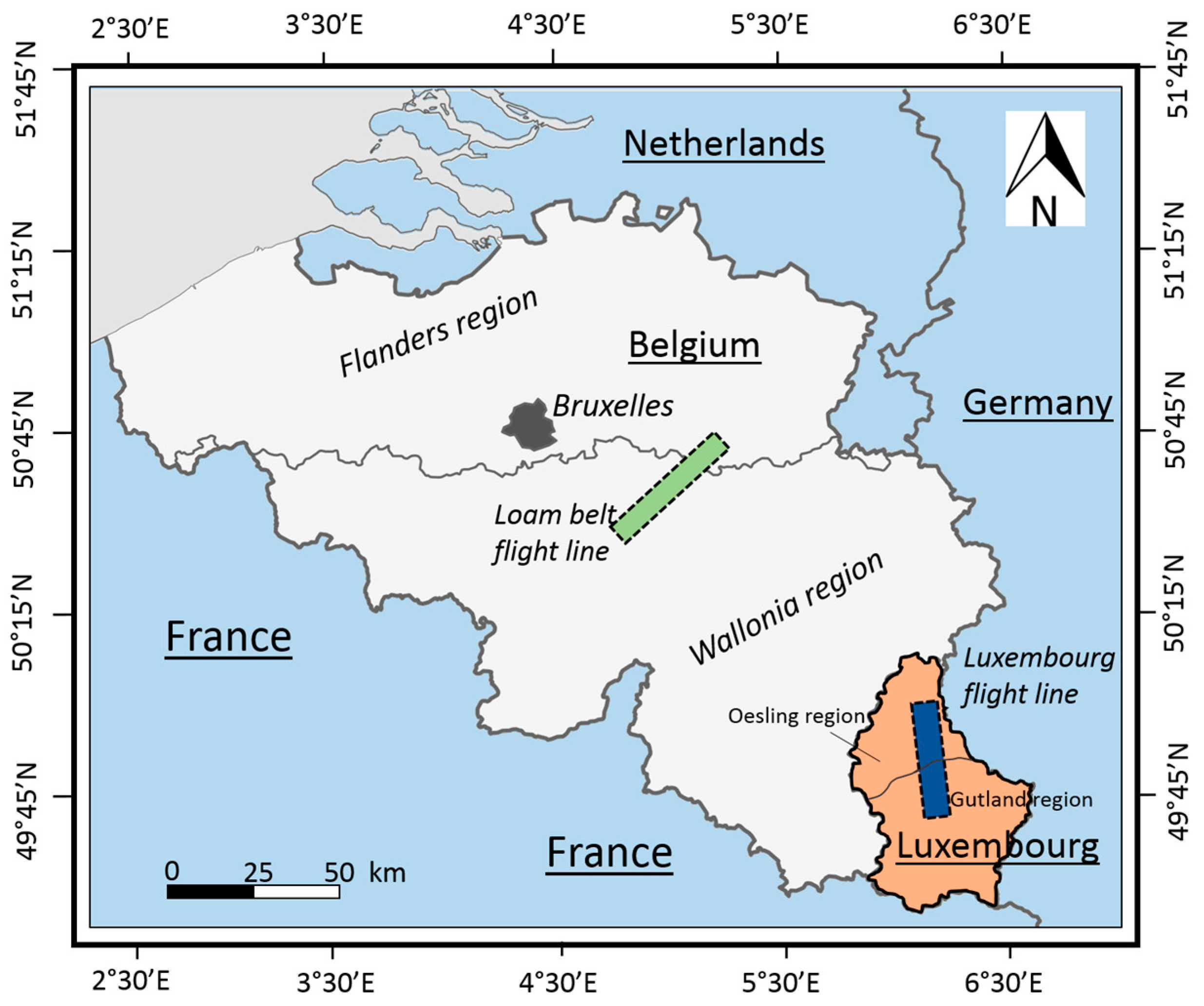
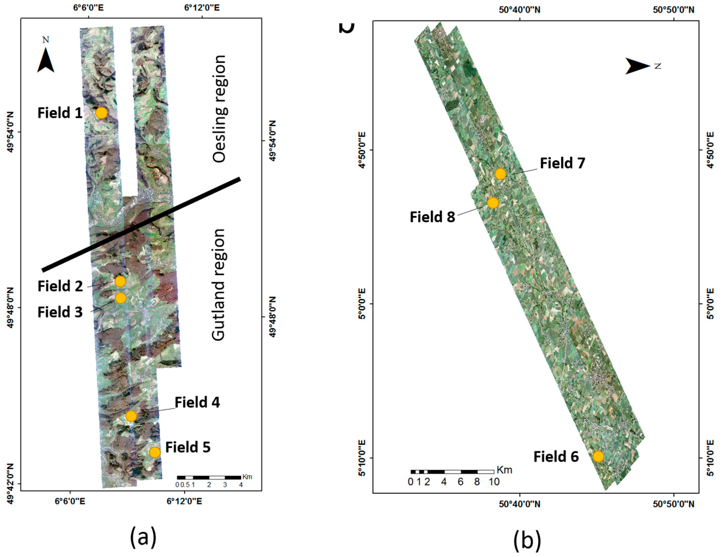
2. Study Area
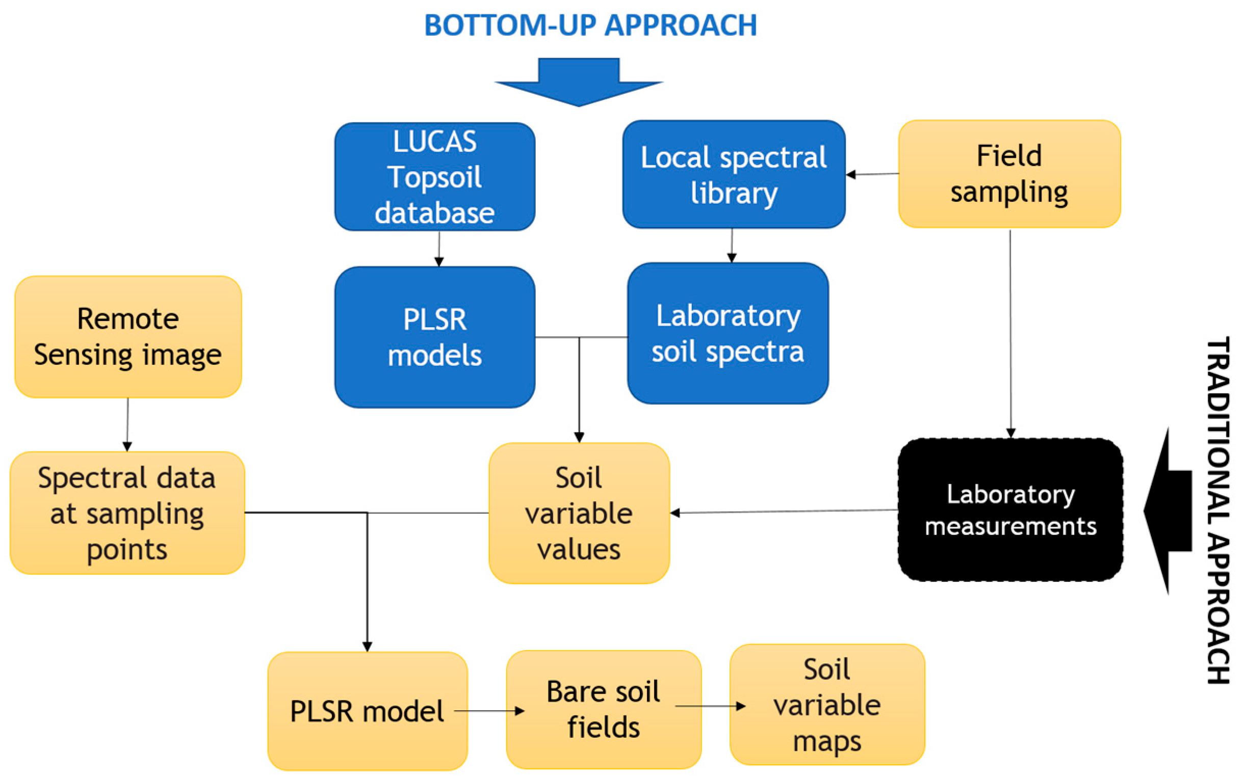
3. Materials and Methods
3.1. Lucas Topsoil Database
3.2. Airborne Images
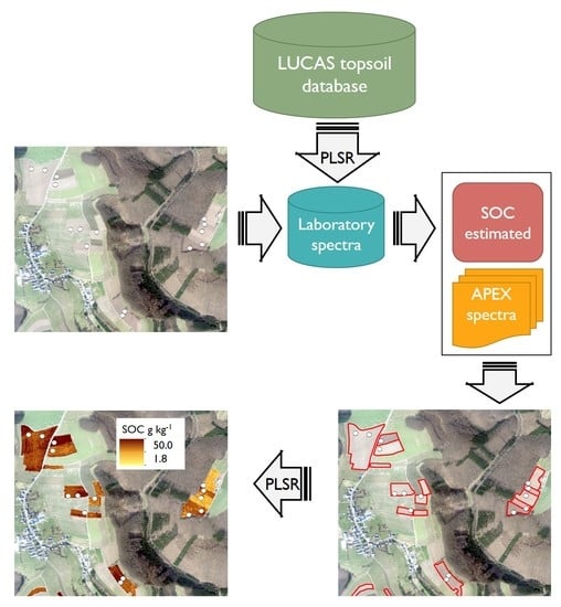
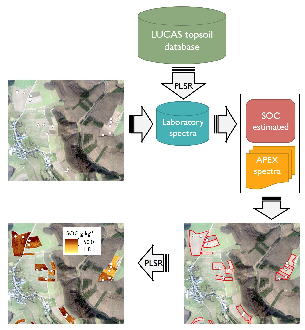
3.3. Soil Organic Carbon (SOC) Estimation
3.4. The Calibration and the Independent Validation Datasets
4. Results
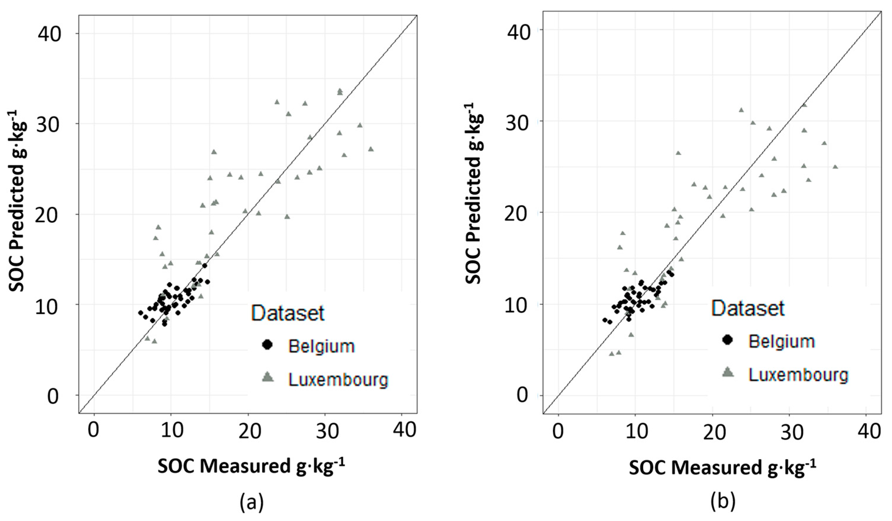
4.1. Calibration and Validation Datasets
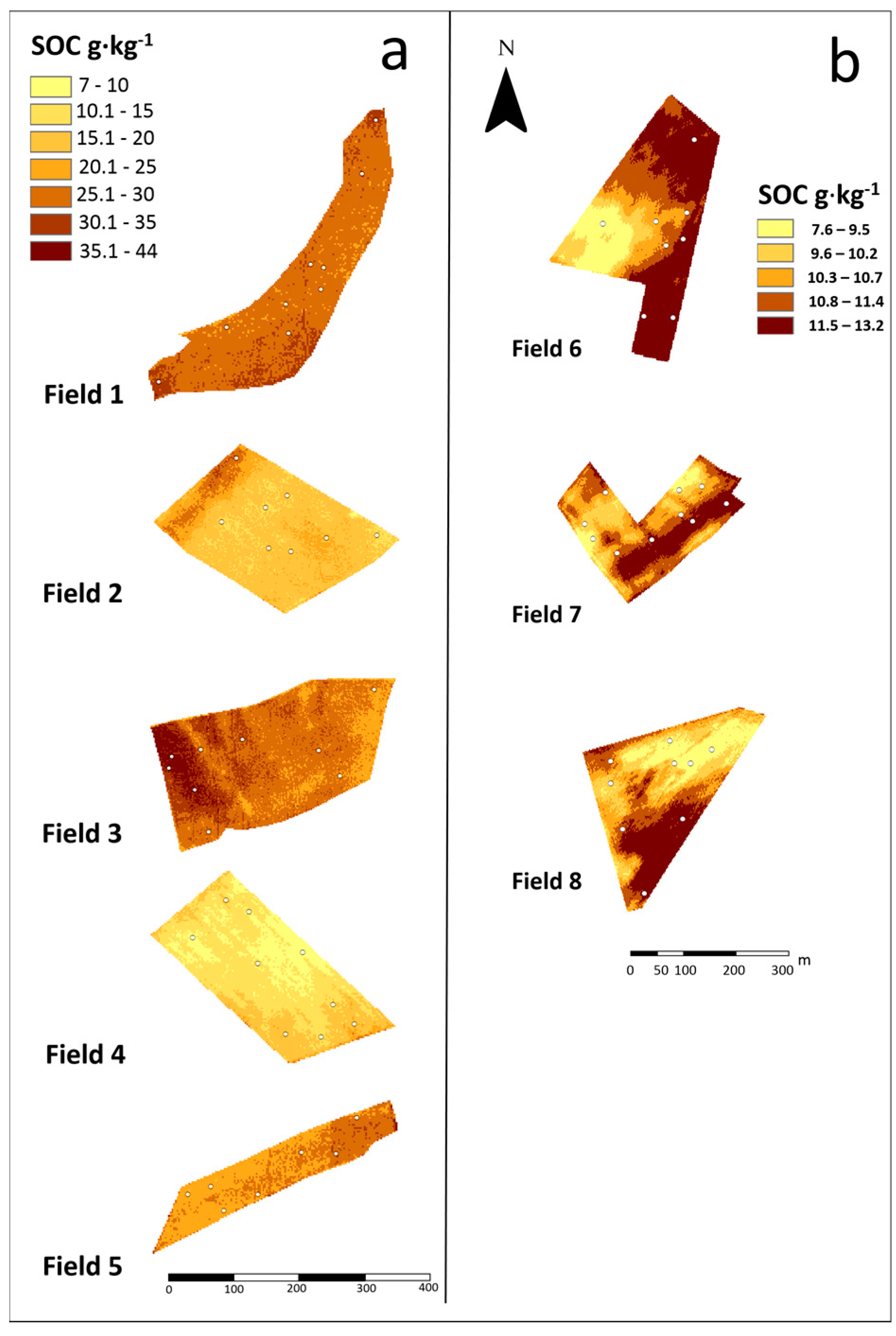
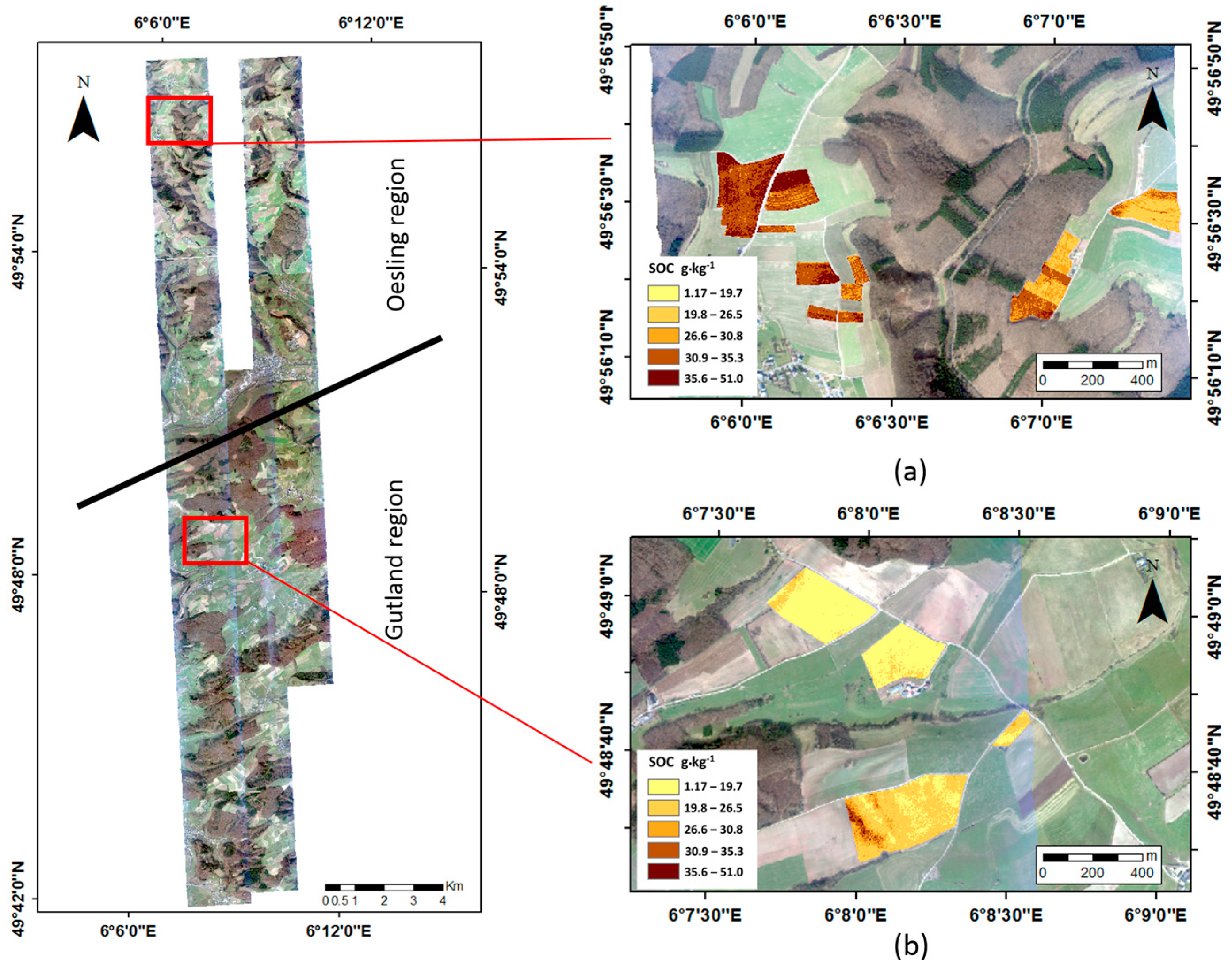
4.2. SOC Estimation
5. Discussion
6. Conclusions
Acknowledgments
Author Contributions
Conflicts of Interest
References
- Chabrillat, S.; Goetz, A.F.; Krosley, L.; Olsen, H.W. Use of hyperspectral images in the identification and mapping of expansive clay soils and the role of spatial resolution. Remote Sens. Environ. 2002, 82, 431–445. [Google Scholar] [CrossRef]
- Castaldi, F.; Palombo, A.; Pascucci, S.; Pignatti, S.; Santini, F.; Casa, R. Reducing the Influence of Soil Moisture on the Estimation of Clay from Hyperspectral Data: A Case Study Using Simulated PRISMA Data. Remote Sens. 2015, 7, 15561–15582. [Google Scholar] [CrossRef]
- Ben-Dor, E.; Inbar, Y.; Chen, Y. The Reflectance Spectra of Organic Matter in the Visible Near-Infrared and Short Wave Infrared Region (400–2500 nm) during a Controlled Decomposition Process. Remote Sens. Environ. 1997, 61, 1–15. [Google Scholar] [CrossRef]
- He, T.; Wang, J.; Lin, Z.; Cheng, Y. Spectral features of soil organic matter. Geo-Spat. Inf. Sci. 2009, 12, 33–40. [Google Scholar] [CrossRef]
- Mouazen, A.M.; Maleki, M.R.; De Baerdemaeker, J.; Ramon, H. On-line measurement of some selected soil properties using a VIS–NIR sensor. Soil Tillage Res. 2007, 93, 13–27. [Google Scholar] [CrossRef]
- Rossel, R.A.V.; Behrens, T. Using data mining to model and interpret soil diffuse reflectance spectra. Geoderma 2010, 158, 46–54. [Google Scholar] [CrossRef]
- Ben-Dor, E.; Chabrillat, S.; Dematte, J.A.M.; Taylor, G.R.; Hill, J.; Whiting, M.L.; Sommer, S. Using Imaging Spectroscopy to study soil properties. Remote Sens. Environ. 2009, 113, S38–S55. [Google Scholar] [CrossRef]
- Wold, S.; Sjöström, M.; Eriksson, L. PLS-regression: A basic tool of chemometrics. Chemom. Intell. Lab. Syst. 2001, 58, 109–130. [Google Scholar] [CrossRef]
- Castaldi, F.; Palombo, A.; Santini, F.; Pascucci, S.; Pignatti, S.; Casa, R. Evaluation of the potential of the current and forthcoming multispectral and hyperspectral imagers to estimate soil texture and organic carbon. Remote Sens. Environ. 2016, 179, 54–65. [Google Scholar] [CrossRef]
- Selige, T.; Böhner, J.; Schmidhalter, U. High resolution topsoil mapping using hyperspectral image and field data in multivariate regression modeling procedures. Geoderma 2006, 136, 235–244. [Google Scholar] [CrossRef]
- Stevens, A.; van Wesemael, B.; Bartholomeus, H.; Rosillon, D.; Tychon, B.; Ben-Dor, E. Laboratory, field and airborne spectroscopy for monitoring organic carbon content in agricultural soils. Geoderma 2008, 144, 395–404. [Google Scholar] [CrossRef]
- Gomez, C.; Lagacherie, P.; Coulouma, G. Regional predictions of eight common soil properties and their spatial structures from hyperspectral Vis–NIR data. Geoderma 2012, 189, 176–185. [Google Scholar] [CrossRef]
- Hbirkou, C.; Pätzold, S.; Mahlein, A.-K.; Welp, G. Airborne hyperspectral imaging of spatial soil organic carbon heterogeneity at the field-scale. Geoderma 2012, 175, 21–28. [Google Scholar] [CrossRef]
- Stevens, A.; Miralles, I.; van Wesemael, B. Soil Organic Carbon Predictions by Airborne Imaging Spectroscopy: Comparing Cross-Validation and Validation. Soil Sci. Soc. Am. J. 2012, 76, 2174–2183. [Google Scholar] [CrossRef]
- Pascucci, S.; Casa, R.; Belviso, C.; Palombo, A.; Pignatti, S.; Castaldi, F. Estimation of soil organic carbon from airborne hyperspectral thermal infrared data: A case study. Eur. J. Soil Sci. 2014, 65, 865–875. [Google Scholar] [CrossRef]
- Steinberg, A.; Chabrillat, S.; Stevens, A.; Segl, K.; Foerster, S. Prediction of Common Surface Soil Properties Based on Vis-NIR Airborne and Simulated EnMAP Imaging Spectroscopy Data: Prediction Accuracy and Influence of Spatial Resolution. Remote Sens. 2016, 8, 613. [Google Scholar] [CrossRef]
- Liu, H.; Shi, T.; Chen, Y.; Wang, J.; Fei, T.; Wu, G. Improving Spectral Estimation of Soil Organic Carbon Content through Semi-Supervised Regression. Remote Sens. 2017, 9, 29. [Google Scholar] [CrossRef]
- Kruse, F.A.; Boardman, J.W.; Huntington, J.F. Comparison of airborne hyperspectral data and eo-1 hyperion for mineral mapping. IEEE Trans. Geosci. Remote Sens. 2003, 41, 1388–1400. [Google Scholar] [CrossRef]
- Castaldi, F.; Casa, R.; Castrignanò, A.; Pascucci, S.; Palombo, A.; Pignatti, S. Estimation of soil properties at the field scale from satellite data: A comparison between spatial and non-spatial techniques. Eur. J. Soil Sci. 2014, 65, 842–851. [Google Scholar] [CrossRef]
- Villafranca, A.G.; Corbera, J.; Martín, F.; Marchán, J.F. Limitations of Hyperspectral Earth Observation on Small Satellites. J. Small Satell. 2012, 1, 19–29. [Google Scholar]
- Casa, R.; Castaldi, F.; Pascucci, S.; Basso, B.; Pignatti, S. Geophysical and Hyperspectral Data Fusion Techniques for In-Field Estimation of Soil Properties. Vadose Zone J. 2013, 12. [Google Scholar] [CrossRef]
- Casa, R.; Castaldi, F.; Pascucci, S.; Palombo, A.; Pignatti, S. A comparison of sensor resolution and calibration strategies for soil texture estimation from hyperspectral remote sensing. Geoderma 2013, 197, 17–26. [Google Scholar] [CrossRef]
- Zhang, T.; Li, L.; Zheng, B. Estimation of agricultural soil properties with imaging and laboratory spectroscopy. J. Appl. Remote Sens. 2013, 7, 073587. [Google Scholar] [CrossRef]
- Guanter, L.; Kaufmann, H.; Segl, K.; Foerster, S.; Rogass, C.; Chabrillat, S.; Kuester, T.; Hollstein, A.; Rossner, G.; Chlebek, C.; et al. The EnMAP Spaceborne Imaging Spectroscopy Mission for Earth Observation. Remote Sens. 2015, 7, 8830–8857. [Google Scholar] [CrossRef] [Green Version]
- Pignatti, S.; Acito, N.; Amato, U.; Casa, R.; Castaldi, F.; Coluzzi, R.; De Bonis, R.; Diani, M.; Imbrenda, V.; Laneve, G.; et al. Environmental products overview of the Italian hyperspectral prisma mission: The SAP4PRISMA project. In Proceedings of the 2015 IEEE International Geoscience and Remote Sensing Symposium (IGARSS), Milan, Italy, 26–31 July 2015; pp. 3997–4000. [Google Scholar]
- Houborg, R.; Anderson, M.; Gao, F.; Schull, M.; Cammalleri, C. Monitoring water and carbon fluxes at fine spatial scales using HyspIRI-like measurements. In Proceedings of the 2012 IEEE International Geoscience and Remote Sensing Symposium, Munich, Germany, 22–27 July 2012; pp. 7302–7305. [Google Scholar]
- Tanii, J.; Iwasaki, A.; Kawashima, T.; Inada, H. Results of evaluation model of Hyperspectral Imager Suite (HISUI). In Proceedings of the 2012 IEEE International Geoscience and Remote Sensing Symposium, Munich, Germany, 22–27 July 2012; pp. 131–134. [Google Scholar]
- Staenz, K.; Mueller, A.; Heiden, U. Overview of terrestrial imaging spectroscopy missions. In Proceedings of the 2013 IEEE International Geoscience and Remote Sensing Symposium—IGARSS, Melbourne, Australia, 21–26 July 2013; pp. 3502–3505. [Google Scholar]
- Gomez, C.; Viscarra Rossel, R.A.; McBratney, A.B. Soil organic carbon prediction by hyperspectral remote sensing and field vis-NIR spectroscopy: An Australian case study. Geoderma 2008, 146, 403–411. [Google Scholar] [CrossRef]
- Shepherd, K.D.; Walsh, M.G. Development of Reflectance Spectral Libraries for Characterization of Soil Properties. Soil Sci. Soc. Am. J. 2002, 66, 988–998. [Google Scholar] [CrossRef]
- Knadel, M.; Deng, F.; Thomsen, A.; Greve, M. Development of a Danish national Vis-NIR soil spectral library for soil organic carbon determination. In Digital Soil Assessments and Beyond; CRC Press: Boca Raton, FL, USA, 2012; pp. 403–408. [Google Scholar]
- Peng, Y.; Knadel, M.; Gislum, R.; Deng, F.; Norgaard, T.; Wollesen de Jonge, L.; Moldrup, P.; Humlekrog Greve, M. Predicting soil organic carbon at field scale using a national soil spectral library. J. Near Infrared Spectrosc. 2013, 21, 213–222. [Google Scholar] [CrossRef]
- Guerrero, C.; Wetterlind, J.; Stenberg, B.; Mouazen, A.M.; Gabarrón-Galeote, M.A.; Ruiz-Sinoga, J.D.; Zornoza, R.; Viscarra Rossel, R.A. Do we really need large spectral libraries for local scale SOC assessment with NIR spectroscopy? Soil Tillage Res. 2016, 155, 501–509. [Google Scholar] [CrossRef]
- Garrity, D.; Bindraban, P. ICRAF A Globally Distributed Soil Spectral Library Visible Near Infrared Diffuse Reflectance Spectra; ICRAF (World Agroforestry Centre)/ISRIC (World Soil Information) Spectral Library: Nairobi, Kenya, 2015. [Google Scholar]
- Tóth, G.; Jones, A.; Montanarella, L. The LUCAS topsoil database and derived information on the regional variability of cropland topsoil properties in the European Union. Environ. Monit. Assess. 2013, 185, 7409–7425. [Google Scholar] [CrossRef] [PubMed]
- Viscarra Rossel, R.A.; Behrens, T.; Ben-Dor, E.; Brown, D.J.; Demattê, J.A.M.; Shepherd, K.D.; Shi, Z.; Stenberg, B.; Stevens, A.; Adamchuk, V.; et al. A global spectral library to characterize the world’s soil. Earth-Sci. Rev. 2016, 155, 198–230. [Google Scholar] [CrossRef] [Green Version]
- Castaldi, F.; Chabrillat, S.; Chartin, C.; Genot, V.; Jones, A.R.; van Wesemael, B. Using LUCAS topsoil database to estimate soil organic carbon content in croplands sampled in Belgium and Luxembourg. Eur. J. Soil Sci. 2017, 19, 6383. [Google Scholar]
- Shenk, J.S.; Westerhaus, M.O. New Standardization and Calibration Procedures for Nirs Analytical Systems. Crop Sci. 1991, 31, 1694–1696. [Google Scholar] [CrossRef]
- Bouveresse, E.; Massart, D.L. Standardisation of near-infrared spectrometric instruments: A review. Vib. Spectrosc. 1996, 11, 3–15. [Google Scholar] [CrossRef]
- Fearn, T. Standardisation and calibration transfer for near infrared instruments: A review. J. Near Infrared Spec. 2001, 9, 229–244. [Google Scholar] [CrossRef]
- Brown, D.J. Using a global VNIR soil-spectral library for local soil characterization and landscape modeling in a 2nd-order Uganda watershed. Geoderma 2007, 140, 444–453. [Google Scholar] [CrossRef]
- Minasny, B.; McBratney, A.B.; Bellon-Maurel, V.; Roger, J.-M.; Gobrecht, A.; Ferrand, L.; Joalland, S. Removing the effect of soil moisture from NIR diffuse reflectance spectra for the prediction of soil organic carbon. Geoderma 2011, 167, 118–124. [Google Scholar] [CrossRef]
- Kopačková, V.; Ben-Dor, E. Normalizing reflectance from different spectrometers and protocols with an internal soil standard. Int. J. Remote Sens. 2016, 37, 1276–1290. [Google Scholar] [CrossRef]
- Schwanghart, W.; Jarmer, T. Linking spatial patterns of soil organic carbon to topography—A case study from south-eastern Spain. Geomorphology 2011, 126, 252–263. [Google Scholar] [CrossRef]
- Nouri, M.; Gomez, C.; Gorretta, N.; Roger, J.-M. Clay content mapping from airborne hyperspectral Vis-NIR data by transferring a laboratory regression model. Geoderma 2017, 298, 54–66. [Google Scholar] [CrossRef]
- Stevens, A.; Udelhoven, T.; Denis, A.; Tychon, B.; Lioy, R.; Hoffmann, L.; van Wesemael, B. Measuring soil organic carbon in croplands at regional scale using airborne imaging spectroscopy. Geoderma 2010, 158, 32–45. [Google Scholar] [CrossRef]
- Goidts, E.; van Wesemael, B. Regional assessment of soil organic carbon changes under agriculture in Southern Belgium (1955–2005). Geoderma 2007, 141, 341–354. [Google Scholar] [CrossRef]
- Sherrod, L.A.; Dunn, G.; Peterson, G.A.; Kolberg, R.L. Inorganic Carbon Analysis by Modified Pressure-Calcimeter Method. Soil Sci. Soc. Am. J. 2002, 66, 299–305. [Google Scholar] [CrossRef]
- Hartigan, J.A.; Wong, M.A. Algorithm AS 136: A K-Means Clustering Algorithm. Appl. Stat. 1979, 28, 100–108. [Google Scholar] [CrossRef]
- Vreys, K.; Iordache, M.-D.; Bomans, B.; Meuleman, K. Data acquisition with the APEX hyperspectral sensor. Misc. Geogr. 2016, 20, 5–10. [Google Scholar] [CrossRef]
- Biesemans, J.; Sterckx, S.; Knaeps, E.; Vreys, K.; Adriaensen, S.; Hooy-berghs, J.; Meuleman, K.; Kempeneers, P.; Deronde, B.; Everaerts, J.; et al. Image processing workflows for airborne remote sensing. In Proceedings of the 5th EARSeL Workshop on Imaging Spectroscopy, Bruges, Belgium, 23–25 April 2007. [Google Scholar]
- Gege, P.; Fries, J.; Haschberger, P.; Schötz, P.; Schwarzer, H.; Strobl, P.; Suhr, B.; Ulbrich, G.; Jan Vreeling, W. Calibration facility for airborne imaging spectrometers. ISPRS J. Photogramm. Remote Sens. 2009, 64, 387–397. [Google Scholar] [CrossRef]
- Vreys, K.; Iordache, M.-D.; Biesemans, J.; Meuleman, K. Geometric correction of APEX hyperspectral data. Misc. Geogr. 2016, 20, 11–15. [Google Scholar] [CrossRef]
- De Haan, J.F.; Hovenier, J.W.; Kokke, J.M.M.; van Stokkom, H.T.C. Removal of atmospheric influences on satellite-borne imagery: A radiative transfer approach. Remote Sens. Environ. 1991, 37, 1–21. [Google Scholar] [CrossRef]
- Haan, J.F.; Kokke, J.M.M. Remote sensing algorithm development. In Operationalization of Atmospheric Correction Methods for Tidal and Inland Waters; Toolkit, I., Ed.; Netherlands Remote Sensing Board (BCRS): Delft, The Netherlands, 1996; ISBN 9789054112044. [Google Scholar]
- Mulder, V.L.; de Bruin, S.; Schaepman, M.E.; Mayr, T.R. The use of remote sensing in soil and terrain mapping—A review. Geoderma 2011, 162, 1–19. [Google Scholar] [CrossRef]
- Savitzky, A.; Golay, M.J.E. Smoothing and differentiation of data by simplified least squares procedures. Anal. Chem. 1964, 36, 1627–1639. [Google Scholar] [CrossRef]
- Nocita, M.; Stevens, A.; Toth, G.; Panagos, P.; van Wesemael, B.; Montanarella, L. Prediction of soil organic carbon content by diffuse reflectance spectroscopy using a local partial least square regression approach. Soil Biol. Biochem. 2014, 68, 337–347. [Google Scholar] [CrossRef]
- Clairotte, M.; Grinand, C.; Kouakoua, E.; Thébault, A.; Saby, N.P.A.; Bernoux, M.; Barthès, B.G. National calibration of soil organic carbon concentration using diffuse infrared reflectance spectroscopy. Geoderma 2016, 276, 41–52. [Google Scholar] [CrossRef]
- Nocita, M.; Stevens, A.; van Wesemael, B.; Aitkenhead, M.; Bachmann, M.; Barthès, B.; Ben Dor, E.; Brown, D.J.; Clairotte, M.; Csorba, A.; et al. Soil Spectroscopy: An Alternative to Wet Chemistry for Soil Monitoring; Academic Press Inc.: Cambridge, MA, USA, 2015; Volume 132, pp. 139–159. ISBN 9780128021354. [Google Scholar]
- Woodcock, C.E. Uncertainty in Remote Sensing. In Uncertainty in Remote Sensing and GIS; John Wiley & Sons, Ltd.: Chichester, UK, 2006; pp. 19–24. ISBN 9780470035269. [Google Scholar]
- Bradley, K.C.; Bowen, S.; Gross, K.C.; Marciniak, M.A.; Perram, G.P. Imaging Fourier transform spectrometry of jet engine exhaust with the telops FIRST-MWE. In Proceedings of the 2009 IEEE Aerospace Conference, Big Sky, MT, USA, 7–14 March 2009; pp. 1–8. [Google Scholar]
- Kanning, M.; Siegmann, B.; Jarmer, T. Regionalization of Uncovered Agricultural Soils Based on Organic Carbon and Soil Texture Estimations. Remote Sens. 2016, 8, 927. [Google Scholar] [CrossRef]


| LUCAS_Crop Class | Textural Class | pH | SOC g·kg−1 | N g·kg−1 | P mg·kg−1 | K g·kg−1 | CaCO3 g·kg−1 |
|---|---|---|---|---|---|---|---|
| A | Loam | 7.2 | 29.7 | 2.8 | 106.5 | 764.2 | 54.5 |
| B | Sandy loam | 5.6 | 21.5 | 1.8 | 43.8 | 111.9 | 0.4 |
| C | Silt loam | 6 | 25.7 | 2.3 | 33 | 168.1 | 1.2 |
| D | Organic soil | 6 | 318.6 | 18 | 34.4 | 193.5 | 11.3 |
| E | Clay loam | 8 | 16.9 | 1.5 | 21.5 | 283.4 | 391.8 |
| F | Sandy loam | 7.4 | 15.8 | 1.5 | 27.9 | 165.8 | 30.9 |
| G | Silty clay loam | 7.5 | 25.1 | 2.4 | 25.8 | 326.4 | 60.8 |
| Dataset | N° | Minimum | Maximum | Mean | Std |
|---|---|---|---|---|---|
| /g·kg−1 | /g·kg−1 | /g·kg−1 | /g·kg−1 | ||
| Calibration | |||||
| Luxembourg | 84 | 6.6 | 49.9 | 23.4 | 11.1 |
| Loam belt | 54 | 7.1 | 15.5 | 10.2 | 1.7 |
| Validation | |||||
| Luxembourg | 43 | 6.9 | 36.0 | 18.9 | 8.6 |
| Loam belt | 45 | 6.1 | 14.7 | 10.2 | 2.1 |
| Traditional Approach | Bottom-Up Approach | |||||
|---|---|---|---|---|---|---|
| Validation Dataset | Calibration Dataset | Validation Dataset | ||||
| RMSE g·kg−1 | RPD | RMSE g·kg−1 | RPD | RMSE g·kg−1 | RPD | |
| Luxembourg | 4.9 | 1.7 | 5.4 | 2.1 | 4.9 | 1.7 |
| Loam belt | 1.5 | 1.4 | 1.2 | 1.4 | 1.5 | 1.4 |
| Total | 3.6 | 2.1 | 4.3 | 2.5 | 3.6 | 2.1 |
© 2018 by the authors. Licensee MDPI, Basel, Switzerland. This article is an open access article distributed under the terms and conditions of the Creative Commons Attribution (CC BY) license (http://creativecommons.org/licenses/by/4.0/).
Share and Cite
Castaldi, F.; Chabrillat, S.; Jones, A.; Vreys, K.; Bomans, B.; Van Wesemael, B. Soil Organic Carbon Estimation in Croplands by Hyperspectral Remote APEX Data Using the LUCAS Topsoil Database. Remote Sens. 2018, 10, 153. https://doi.org/10.3390/rs10020153
Castaldi F, Chabrillat S, Jones A, Vreys K, Bomans B, Van Wesemael B. Soil Organic Carbon Estimation in Croplands by Hyperspectral Remote APEX Data Using the LUCAS Topsoil Database. Remote Sensing. 2018; 10(2):153. https://doi.org/10.3390/rs10020153
Chicago/Turabian StyleCastaldi, Fabio, Sabine Chabrillat, Arwyn Jones, Kristin Vreys, Bart Bomans, and Bas Van Wesemael. 2018. "Soil Organic Carbon Estimation in Croplands by Hyperspectral Remote APEX Data Using the LUCAS Topsoil Database" Remote Sensing 10, no. 2: 153. https://doi.org/10.3390/rs10020153