1. Introduction
Assessment and monitoring of forests’ growing stock is important for sustainable use of forest resources, planning investments in forest sector and mitigating effects of climate change. Forests’ growing stock is systematically monitored with different kinds of forest inventory methods. For model based forest inventory using remotely sensed data, there are different sources of data that could be applied, such as satellite imagery, aerial photography, airborne laser scanning (ALS) or a combination of these. The choice of the data source used is application-dependent. It depends on the required accuracy and the level of detail in the resulting data and outcomes. The methods based on airborne data are rather complex in terms of practical arrangements, since they require a mission-specific data acquisition campaign. Due to their relatively high accuracy and detailed data deliverables, airborne data are convenient for the purpose of operational, detailed forest management planning. A forest inventory based on satellite imagery is economical for large area mapping, as in the general case, medium-resolution satellite imagery such as Landsat 8 Operational Land Imager (OLI) is freely available. However, a forest inventory based on medium resolution satellite images has lower accuracy than one that is based on airborne measurements [
1], but its accuracy can still be adequate for general forest growing stock assessment at a low spatial resolution. For a concise but comprehensive overview of the relative merits of different remote sensing modalities and estimation methods, please see the review [
2] and references therein.
According to the National Forest inventory guidelines of Russia [
3], the period of repetitive forest data observations is set to 10–15 years. For some of Russia’s forested areas, this recommendation is not always followed, due to remoteness, lack of transport infrastructure, high field work costs, and the low economic value of the forests, considering the overall forest industry development level in such regions. In practice, this means that some of the existing official forest data are extremely outdated, being acquired, e.g., in the 1980s–90s of the 20th century, and they do not consider, for example, recent forest fire events and growth increments. At the very same time, there are a number of forest industry development initiatives that currently require information about the state of the forests, in order to provide efficient investment decisions both on the level of private investors and the government. In most cases, forest industry projects in Russia consider large-size forest concessions, ranging from hundreds of thousands to millions of hectares of forestland. Due to the financial structuring of such projects, it is often required that forest assessment results for an entire area under consideration are delivered in a short time frame, with accurate and objective results. From that point of view, one possible approach is the use of satellite imagery-based forest inventory.
Satellite imagery-based forest inventory is indeed already a rather old technique; the fundamentals of the approach were introduced already in the 90s; see, e.g., [
4,
5]. However, despite the fact that satellite imagery-based forest inventory techniques have been well elaborated, one of the most critical phases of the estimation process, field data acquisition, has not been changing much over time. Field data measurements, on the one hand, influence the quality of the forest inventory results, but on the other hand, a field campaign carries a large portion of the forest inventory campaign’s costs. Typically, employing conventional tools such as calipers and a hypsometer/clinometer in field data acquisition has been rather labor intensive. Furthermore, the approach using conventional tools, in some specific cases, suffers from low objectivity and demands field data cross-validation by revisiting a certain number of sample plots, in order to independently confirm field data quality. Modern-type calipers and hypsometers/clinometers are indeed rather sophisticated tools nowadays; see e.g., [
6], possessing Global Positioning System (GPS) readings that improve the objectivity of the measurements. Also, the accuracy and precision of measurements is expected to be high when trained mensurationists are using the tools [
7]. Even though such tools are advanced equipment, and even though they can provide high accuracy and precision, it is known from their practical application that they remain complex and time consuming, as well as requiring well-trained and experienced field crews. In that specific context, there is a need to employ a field sampling tools that enable faster field campaigns, maintaining a good level of acquired data accuracy, and providing a high level of data objectivity in harsh conditions. Objectivity requirement of the data acquisition can be achieved by automated non-contact field data collection methods. These include terrestrial laser scanning (TLS) [
8,
9,
10] and close-range photogrammetry [
11,
12]. These methods, however, require purpose-built equipment and computationally heavy post-processing, and their performance is related to the complexity of the forest structure, and their measurement accuracy in field tests has not always been convincing. Mobile phone technology offers an alternative to automated field data collection, with a more generally available platform. Mobile devices and applications have been successfully tested in participatory projects for collecting data for forest fuel estimation [
13], in forest monitoring [
14], and in creating forest cover maps [
15]. Besides their use as a data collection device designed for professional and non-professional users, mobile phones can be used as measuring devices. The camera relascope [
16] is an alternative method to automate and streamline field data collection, and to allow non-professionals to participate in data acquisition campaigns.
The idea of using data collected using mobile applications as training data in satellite-based mapping of forest related variables has been introduced in [
13,
15,
16]. In this study, we push the idea forward by testing a commercially available camera relascope tool, Trestima (
www.trestima.com/w/en/) [
17], in collecting field sample data at arbitrary sized sample plots, and we use the collected field data as training data in Landsat 8 OLI based forest inventory in a large area in central Siberia (Russia). Trestima differs from another camera relascope tool, Relasphone, described in [
16] in its level of automatization. While in Relasphone, the user must count the measured trees and define the species for each tree, Trestima detects the species and delivers the basic metrics of a forest stand as basal area, number of stems, and diameter distribution, based on automatic image interpretation.
The way in which this article uses Landsat 8 OLI data is relatively simple. We apply satellite images from two seasons, leaf-on (summer) and leaf-off (spring/autumn) seasons. By this, we aim at a better separation of tree species. However, we would expect further improvements of the results to be obtainable from modern methods that use a time series of satellite images (see e.g., [
18]), or even the difference of heights derived from different space-born instruments, such as the method proposed in [
19].
This study considers the forest inventory for mean volume, basal area, and coniferous/deciduous mapping of a large area in central Siberia, approaching 2.6 million hectares (ha), employing modern camera relascope-based field measurements at arbitrary sized sample plots and medium-resolution freely sourced satellite imagery from Landsat 8 OLI. The applied camera relascope tool was Trestima, which is a commercial and operationally used forest inventory system used mainly in stand-level assessments. The assessment accuracy is evaluated earlier in Finnish conditions for stand-level mapping [
20]. However, the data collected with the tool has not been used for training data in satellite-based inventory.
The objective of the study was to validate the applicability of camera relascope measurements in field plots in the environment of the large-scale forest inventory, and to test the suitability of these field data in medium-resolution satellite-based forest inventory. Also, the study validates the use of Landsat 8 OLI images from different seasons, with the aim to improve estimation accuracy.
2. Materials and Methods
This section and its subsections describe the materials used, and the methods divided in the characterization of the study area, acquisition and processing of input data, data analysis and modeling, and finally the description of the validation methods.
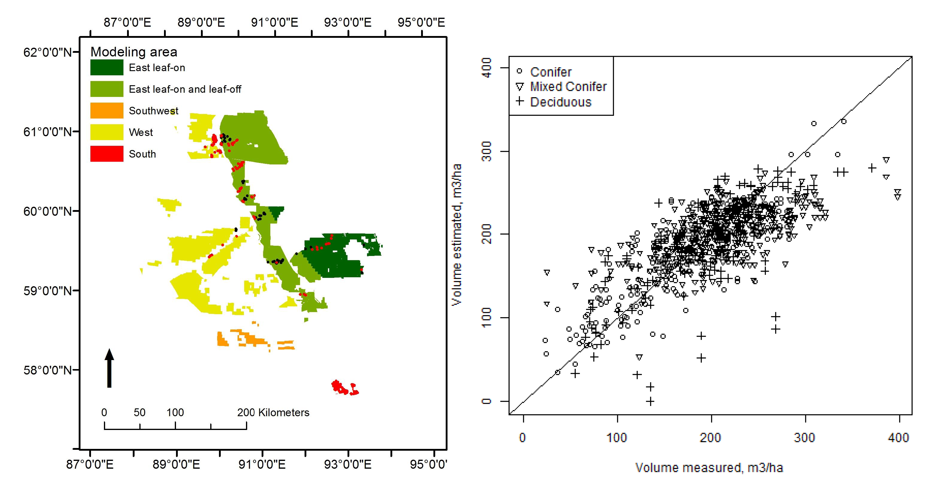
Figure 1 presents a workflow diagram of the whole process.
2.1. Study Area
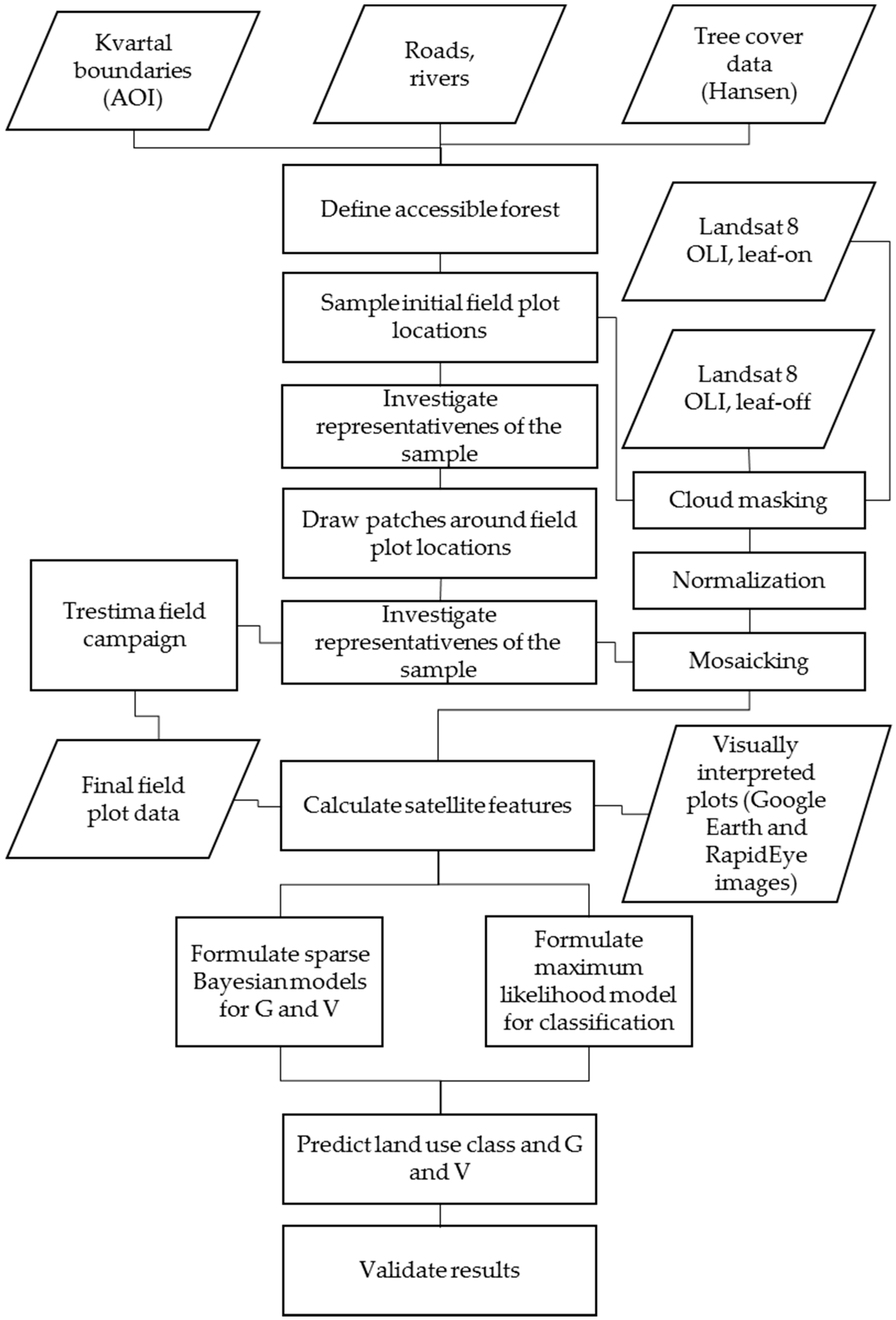
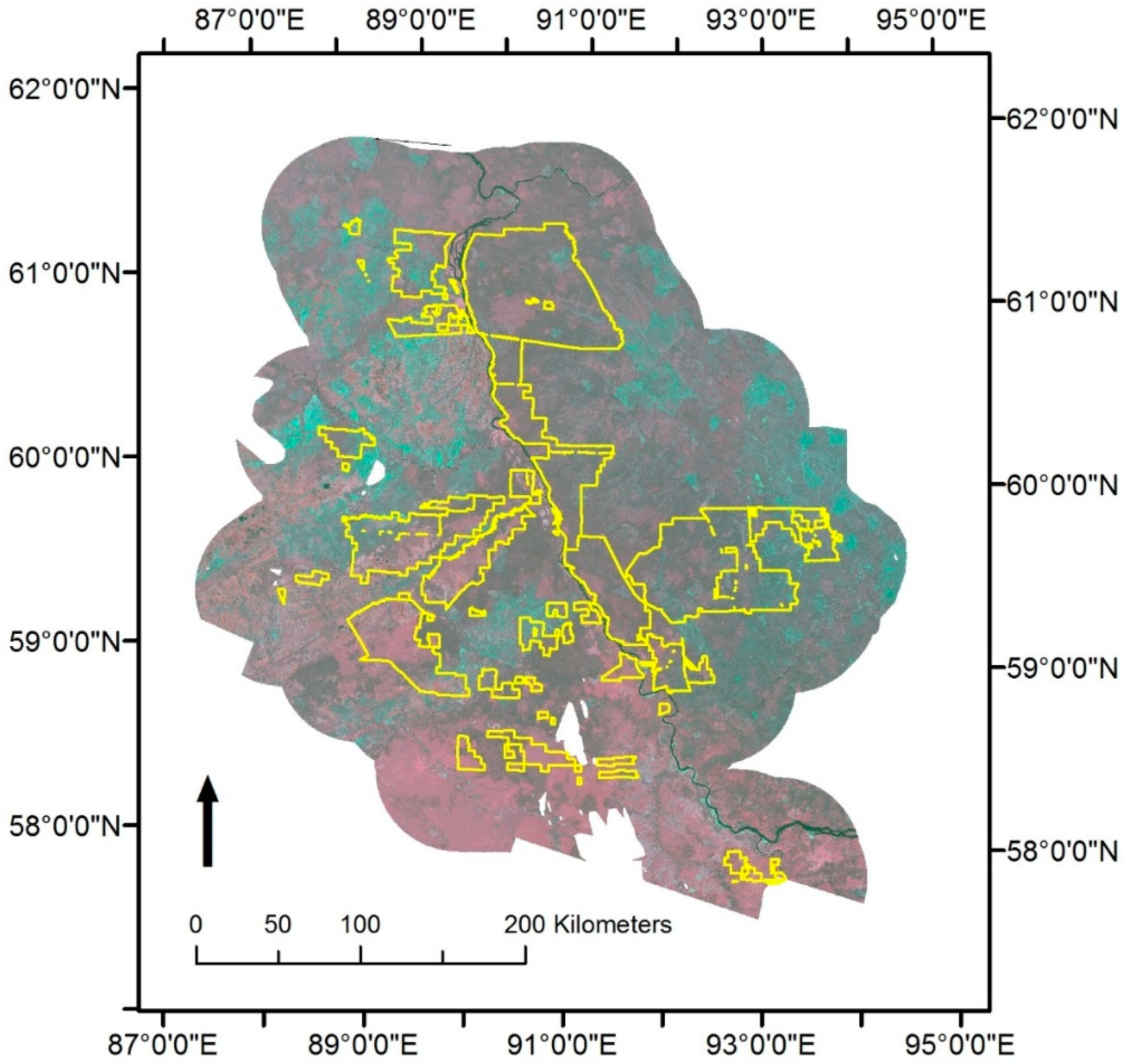
The forest inventory took place in the summer–fall season of 2015. The study area, later the area of interest (AOI), is located in central Siberia (Krasnoyarsk region, Russia); see
Figure 2.
The dimensions of the AOI are approximately 450 km along and 350 km across. In total, the AOI comprises 2,691,316 ha. The AOI is featured by lack of road infrastructure, and mainly represents intact forests (taiga). The AOI consists of forest units, the majority of which has a rectangular form of so-called forest kvartals scattered in either large or small groups and/or lying all along over the territory (see [
21] for the definition of a kvartal). Geographically, the AOI is located in the proximity of the Yenisei river on its west and east banks.
Forests on both banks of the river were represented by the coniferous species of Scots pine (Pinus sylvestris L.), Norway spruce (Picea abies L.), Fir (Abies Mill.), Larch (Larix sibirica Lebed.), Siberian pine (Pinus sibirica Du Tour), and by the deciduous species of Birch (Betula L.) and Aspen (Populus tremula L.), all being of different ages at the different parts of the AOI. The most southern part of the AOI differs from the rest of the area. It has been under exploitative forest use, and deciduous species are more dominant. At the time of the study, actual dominance and distribution of species over the area were not well known. Some parts of the AOI have undergone recent severe forest fires. The environment on the west bank is characterized by a flat terrain of lowlands and widespread swamps. The environment on the east bank of the river is rather mountainous, with elevations of up to 700–900 m above sea level, and characterized by frequent large tributaries of the Yenisei river that penetrate deep into the territory over many kilometers.
2.2. Remote Sensing Data
The remote sensing data employed in the study were cloud-free Landsat 8 OLI imagery of both leaf-on (summer) and leaf-off (autumn) seasons for the entire AOI. Processing level-1 images were obtained from the U.S. Geological Survey, Earth explorer service [
22]. The image search was first conducted for images from 2015 with less than 10% cloud cover; however, the search criteria were later adjusted to include images with higher cloud cover percentages, and the search was expanded to also include the years 2013 and 2014. Leaf-off images were searched from both autumn and spring seasons. Mountainous areas was problematic because of snow cover: suitable leaf-off images were not detected for that area. The downloaded imagery was first analyzed visually using LandsatLook images as aids. This was done to identify the most suitable images, possible mosaicking the order of images, and checking that the images covered the entire area, and also after masking out the clouds. The total number of images used was 18 and 9 for leaf-on and leaf-off mosaics, respectively. Acquisition dates for leaf-on images were 1 July 2014, 12 July 2014, 4 August 2014, 13 August 2014, 6 June 2015, 15 June 2015, 22 June 2015, 25 August 2015, and 1 September 2015. Acquisition dates for leaf-off images were 29 September 2013, 28 September 2014, and 30 September 2014. For further processing, the original 12 bit images were resampled to 32 bit images, because the ArboliDAR tools [
23] used for feature calculation required 32 bit raster data as an input.
The mosaicking of images was done in ArcGIS 10.0 software. Due to variation in satellite image acquisition conditions, the same ground object on two overlapping images can result in different spectral values [
24]. Because of this, radiometrically uniform mosaics using multi-temporal scenes should be created prior to employing the satellite imagery into image analysis. To overcome radiometric differences between the multi-temporal scenes, relative normalization by pre-processing of the input images was performed. Relative radiometric normalization is based on the assumption that the difference between two satellite images from different dates but from the same area can be explained by a linear relationship [
25]. To resolve this problem, we used the variance-preserving mosaic (VPM) algorithm that minimizes the overall error of the normalization, and aims to preserve the average variance of input scenes [
26]. Normalization was done using the VPM algorithm implemented into the ArboLIDAR toolbox, developed by Arbonaut Ltd., Finland [
23]. The normalization procedure utilizes overlapping portions of the images, and prior to normalization, clouded and shadowed areas as well as image edges with black or clearly abnormal pixel values were delineated. Portions of the image that do not contain relevant information and that might affect the normalization negatively, need to be masked out; i.e., pixel values need to be set as No Data. Polygon shapefiles were used as masks. The AOI was buffered by 50 km. Areas further than 50 km from AOI were set as No Data. The black edges of each image needed to be set to No Data. In addition to the black edges, some pixels on the edge of the scenes had abnormal values. Worldwide Reference System (WRS-2) scene boundaries downloaded from U.S. Geological Survey Earth explorer service [
22] were used to remove areas on the edges of composite images. Other masks were created mostly with manual editing. Images were analyzed visually to detect clouds and shadows, or other areas with inferior quality, and then these areas were delineated by hand. For some of the Landsat scenes, LandsatLook quality images were further processed to mask out very scattered small clouds and their shadows. If there were clouds outside the AOI, they needed to be masked out as well, so that they would not affect the normalization result negatively. Several images adjacent to each other had no visible image borders. This was the case, for example, for when the images were from the same date. Based on visual analysis, it was decided that several of the masked composite images could be mosaicked without normalization. These mosaics and other individual composite images were then normalized and mosaicked into one image mosaic covering the entire AOI (
Figure 3).
2.3. Sample Design Plan
Initially, the sample plot design was an L-shaped cluster format with four plots in each cluster. The distance between center coordinates of plots was 200 m. The AOI defined by the rectangular planning compartment, kvartal boundaries, which were preliminarily digitized in GIS shape file format, was divided into two areas—on the west bank and on the east bank of Yenisei, respectively. The forested area was defined by delineating out non-forest areas based on Hansen tree cover data [
27], as well as rivers and roads, with a 100 m buffer. The accessible forest was defined by using roads and rivers (at the field campaign the rivers were also used as transport lines) that were preliminarily evaluated in terms of their usability. The maximum distance from a usable road to a plot was 2000 m, and no rivers could be crossed on the way to the plot. Cluster locations were randomly sampled in accessible forest area. Each initial sample plot was of Landsat 8 OLI -pixel size of 30 × 30 m.
Next, the initial sample plots were compared over the forest area of AOI variation. The aim was to have field data representing the variation of the whole AOI, in order to obtain good estimation accuracy and precision with a low number of field plots; see e.g., [
28,
29,
30]. The representativeness of the initial sample was analyzed by comparing and plotting green, red and NIR (near infrared) band values and NDVI (normalized difference vegetation index) image values from the initial sample plots, and from the whole forested area of the AOI. The values for the whole forest area of AOI were from a large random sample (n = 15,355). The materials used for the analysis were cloud-free image mosaics produced from the best available summer season Landsat 8 OLI images that were obtained before August 2015. Image parts with cloud or cloud shadow were removed and supplemented with data from other images.
Arbitrary sized forest patches around the plot center coordinates were then drawn manually. A patch was not allowed to be in a road or a river and the land use/land cover class, tree species composition and volume were to be visually assessed as being homogeneous inside the patch. When it comes to the volume, the assessment was done in the sense that, provided the land use/land cover class, tree species composition is the same, and then if the patch of forest seemed visually homogeneous, it was assumed that the forest is also similar in volume. Thus, in manual segmentation, a plot could be moved to a more homogeneous location, or removed if it could not be moved. The manual segmentation was performed based on the visual interpretation of Landsat 8 OLI imagery, with the support of satellite imagery available on Google Earth. On average, an arbitrary-sized plot area was set to be approximately 0.5–1 ha (6–12 Landsat 8 OLI pixels), which could vary depending on the homogeneity.
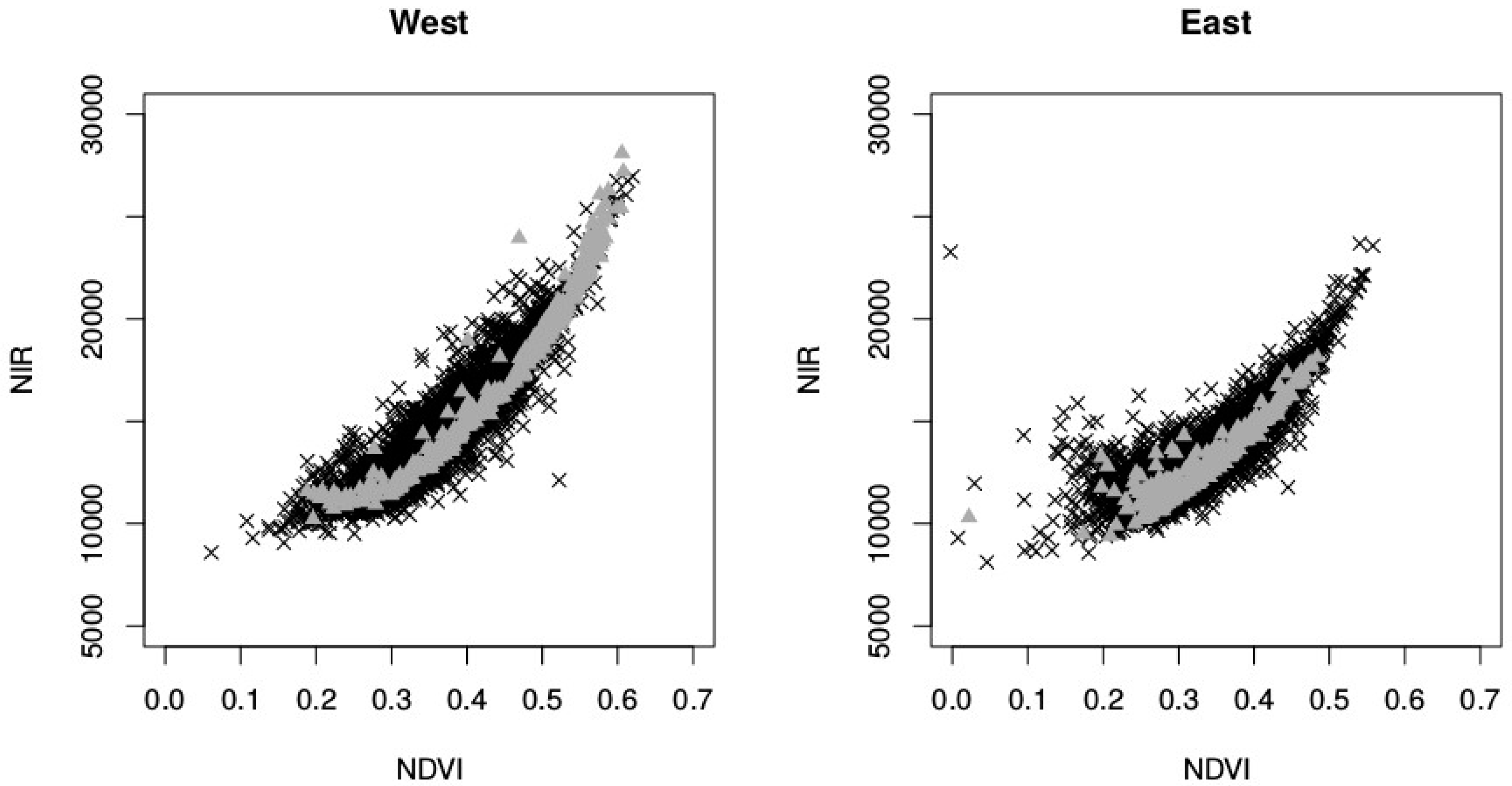
The size of the initial sample was 848 plots, with 424 plots on each side of the river Yenisei. Some of the plots from the initial sample were removed because they were not accessible after reviewing them, based on the information from the field team. After the removal of the inaccessible plots, the revised sample consisted of a total of 792 plots. All in all, 392 and 400 plots were left at the east and west banks of the river Yenisei, respectively. The representativeness of the revised sample against Landsat 8 OLI satellite image spectral values is presented in in
Table 1.
The analysis showed that on the east bank of the river, the revised sample well represented the variation of the whole inventory area. There were some extreme values (e.g., in green and red bands) that were not covered in the sample. It was assumed that these extremes did not represent the forests, but some other land use classes. On the west bank of the river, the sample covered the variation well; however, the means were shifted towards high NIR and NDVI values. Also, the variation of the inventory area differed significantly, compared to the areas on the east bank of the river. The most southern planning compartments (kvartals) were well-represented in the sample, and the rest of the kvartals on the west bank of the river Yenisei were underrepresented. The reason for this was that the accessible area on the west bank was quite limited.
Finally, during manual segmentation, the number of sample plots was reduced to 385 and 399 at the west and east banks of the river Yenisei, respectively, due to some inaccessible plots found in visual interpretation. An average area of a forest patch was 0.8 ha, with a minimum area of 0.4 ha and a maximum area of 1.8 ha. The representativeness of the final sample was investigated by calculating NIR and NDVI values as the mean of pixel values in the patch. This slightly averaged the values compared to the pixel-based method used in analyzing the revised sample. However, the averaging effect was minor, since the patches were segmented in homogeneous areas. The representativeness of the final sample was checked again against the random sample. Scatter plots in
Figure 4 show how NIR and NDVI values of the final sample compared with the random sample presenting the variation in AOI.
2.4. Field Plot Data Acquisition
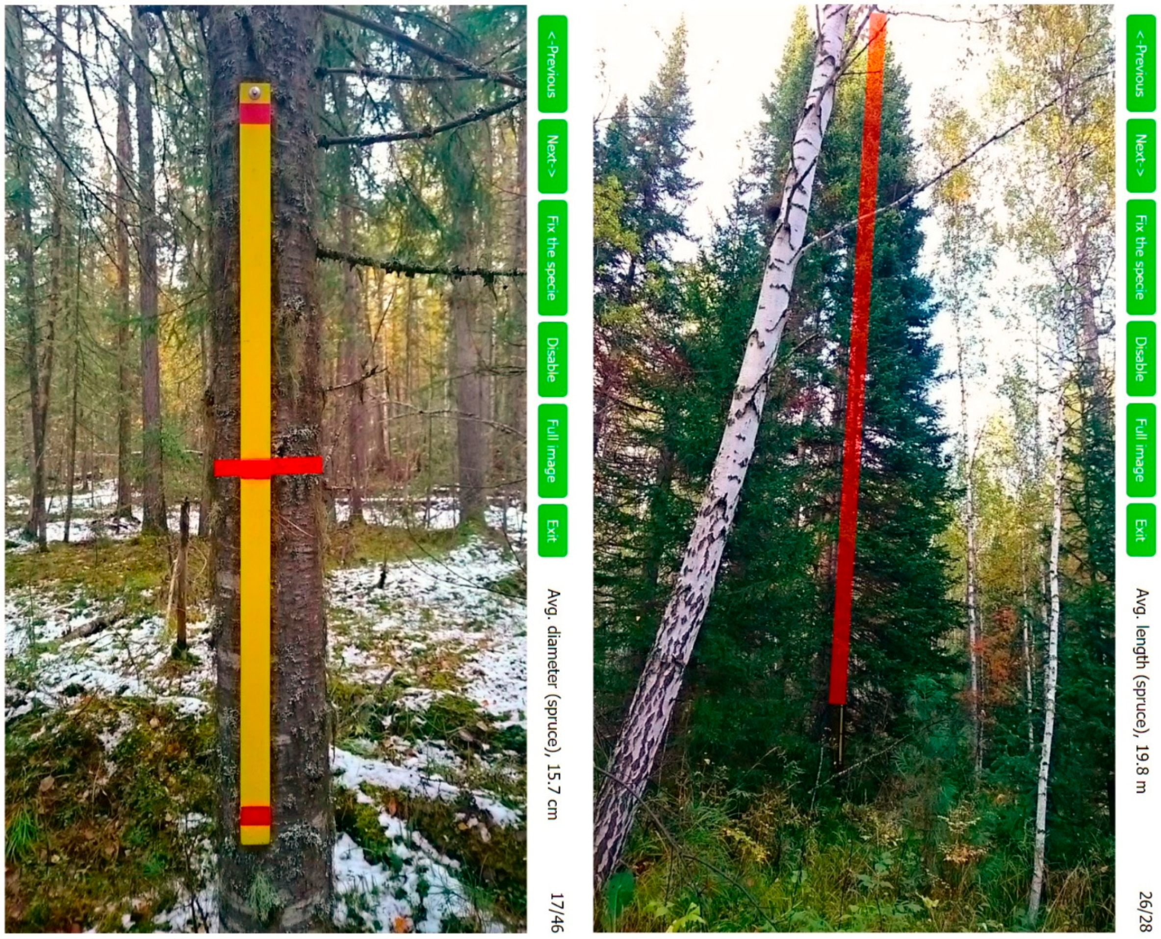
The fieldwork took place in the period between late August and early October 2015. The Trestima camera relascope system was used to measure the field plots. The Trestima camera relascope is a new generation of terrestrial forest inventory tools, which is based on using a mobile application. As input data, Trestima uses terrestrial imagery of two types: basal area images and individual tree images, captured with the mobile application. Trestima automatically detects species and delivers such basic metrics of a forest stand such as basal area, the number of stems, and diameter distribution, which is defined as the number of trees in each diameter class, as well as detecting diameter and height, when trees are measured individually [
31,
32]. Because there was no assured information available on the accuracy of the automatic species detection in the study area, each image at each sample plot was reviewed manually, and if the tree species was wrong, it was changed.
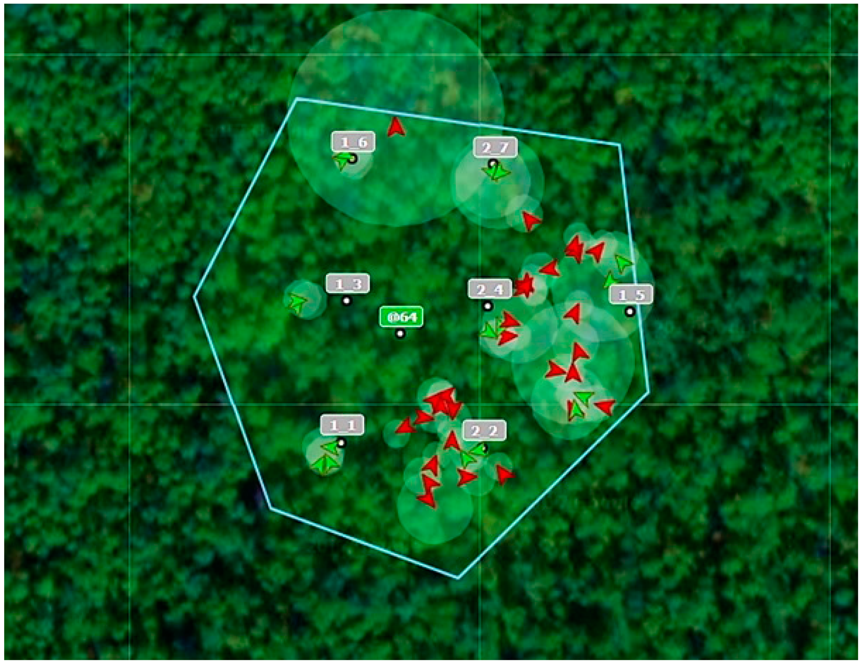
The field work was performed using the mobile phones Sony Xperia Z3 (Android) and Nokia Lumia 720 (Microsoft). Prior to field measurements, each sample plot was covered with a systematic net of points (30 × 30 m). The net was visible on each mobile device. The points in the mobile devices served as navigation orienteers for the field crew. The assignment was to approach to as near as possible at each such point, taking into consideration the local environment and the mobile device’s GPS accuracy, and to capture two sample images of basal area in approximately perpendicular directions inward a sample plot (
Figure 5). On a typical plot, there were seven points, which resulted in 14 basal area images (7 × 2 images). Simultaneously, at each sample plot, the field crew selected a minimum of two model trees per each tree species, and measured the individual trees’ diameter and height (see
Figure 6). This means that the number of model tree images was dependent on how many tree species were present on the plot. The average value of basal area from basal area images was used as the field measured basal area of the plot. Model trees were used for estimating the height–diameter curve. All in all, 16,516 sample images of either type, i.e., the basal area image or the model tree image, were taken from a total of 599 field plots.
By default, Trestima calculates the sample plot volume automatically, based on the basal area sample images from the plot, as well as the height and diameter measurements of subjectively selected trees per tree species. The volumes are calculated using volume models per tree species, configured in Trestima [
31]. However, as the default Trestima volume models were not tailored to this project, the estimation of the forest volume per each sample plot was done using Trestima diameter distribution from each plot, which defined the number of trees on each diameter class by species. Heights were estimated with height–diameter models (h(d)-models) generated from the model tree data, and tree level allometric volume functions specific to the forest region of the AOI were used to calculate diameter class level volumes. The height per tree species was estimated for each diameter class by using h(d)-models estimated for the southern part, and the rest (western, south-western, and eastern) separately. The models were created in the statistical program R [
33] and in the package nlme [
34] using nonlinear mixed-effects modeling. The mixed-effects models were applied for modeling the relationship between tree height and tree diameter, because the variables were clustered and thus spatially correlated, see e.g., [
35]. The plot was used as the random variable in the modeling, assuming that different plots have somewhat different growth conditions, and thus plot affects the h(d)-model curve. The h(d)-models were created separately for each major tree species of the following areas: in the southern part pine, spruce, birch, and aspen each had their own models, and in the western, southwestern, and eastern parts, cedar and other (deciduous) tree species each had their own, in addition to those mentioned before. Some minor tree species data were combined to suitable major tree species groups: in the western, southwestern, and eastern parts larch and fir were merged with spruce, in the southern part, cedar and other species with pine. All h(d)-models were made with the Näslund function [
36] after testing several options.
Finally, the volume of the growing stock per each sample plot was estimated by summing up the volumes of the diameter classes per tree species, which were calculated based on tree-specific allometric volume models [
37], taking as the input data the estimated quantity of the trees of each respective diameter class.
2.5. Land Use Classification
Maximum Likelihood Classification tool in ArcGIS 10.0 toolbox Spatial Analyst was used to classify a Landsat 8 OLI mosaic with supervised maximum likelihood method. The area was classified into nine land use classes (Conifer forest, Mixed conifer forest, Deciduous forest, Swamp, Grass, Harvested, Regrowth, Open land, Water and Burnt area). Training areas consisted of field plots measured with Trestima, and additional training areas established based on visual interpretation by creating several polygons for each land use class. RapidEye satellite imagery and satellite imagery available on Google Earth were used as ancillary information for establishing training areas. An independent random sample of 207 visually interpreted plots was acquired for validation.
2.6. Estimation of Forest Volume and Basal Area
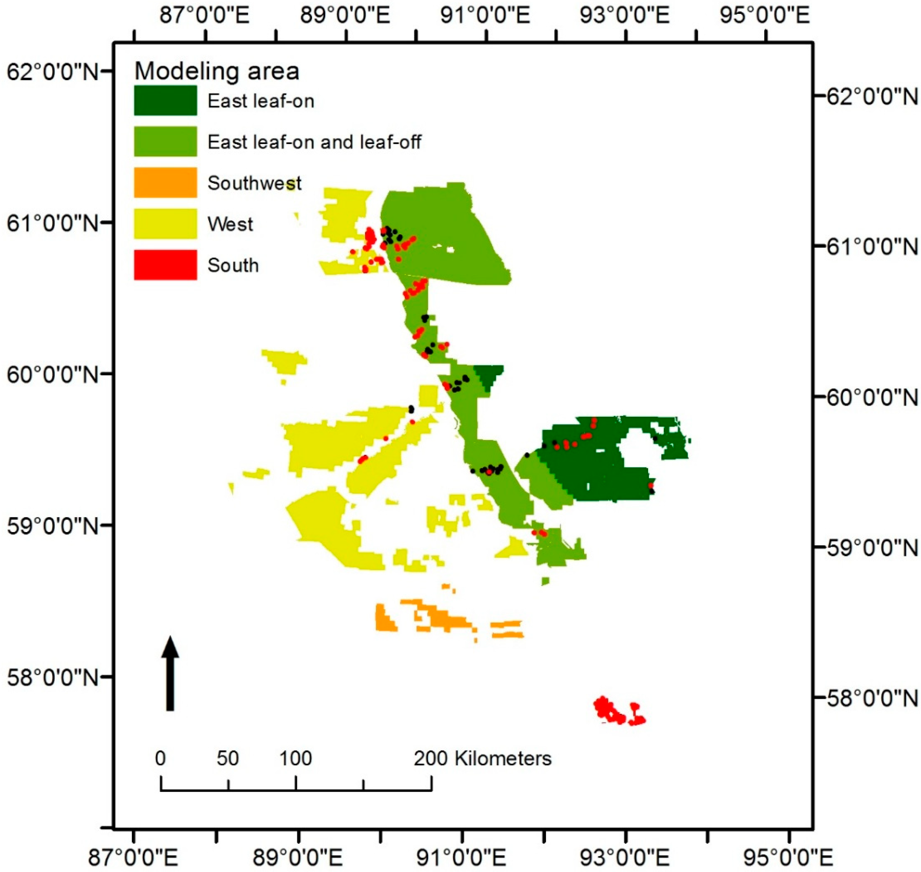
All in all, data from a total of 599 plots were delivered from the field campaign. Of the 599 plots, 544 were used for further modeling. Some plots were left outside modeling, due to poor satellite image quality on the plot region, or due to problems in measurements. The highest possible model quality was assured by not using plots with some quality issues that might distort the models. The forest volume modeling was done separately for the four major parts of the AOI: South, West, Southwest, and East parts (
Figure 7). The division was based on satellite imagery and forest characteristics, i.e., the modeling area was the area with homogenous satellite data and similar forest types (lowlands, mountainous).
The area of each respective part is estimated as follows:
At the estimation, different field plot combinations were used in the different areas. By default, both leaf-on and leaf-off Landsat 8 OLI images were used in models, except for the mountainous area of the east bank, where different image compositions were applied because good quality leaf-off images were not available for the whole area. Also, because of mountains, the East area had large shadowed areas, and therefore, separate shadow area models were estimated. Field data statistics for the modeling areas are presented in
Table 2. The used field plot and Landsat 8 OLI combinations were:
South area (both leaf-on and leaf-off imagery):
- -
228 plots (all plots from the Southern part);
West area (both leaf-on and leaf-off imagery):
- -
119 plots (all plots from the Western part);
Southwest area (both leaf-on and leaf-off imagery):
- -
217 plots (119 of plots from the Western and 76 of plots from the Southern part);
East area:
- -
Leaf-on and leaf-off imagery (model 1): 160 plots;
- -
Leaf-on imagery only (model 2): 160 plots;
- -
Shadowed leaf-on and leaf-off imagery (model 3): 43 plots;
- -
Shadowed leaf-on imagery (model 4): 43 plots.
Models for volume and basal area estimation were built using field plot data and satellite image features calculated for sample plots using Sparse Bayesian Regression (SBR) method [
38,
39]. SBR is a linear regression method, which automatically selects the needed covariates from the set of candidate covariates to estimate a forest variable. By default, in SBR, a specific set of covariates is employed in order to estimate each forest variable.
The modeling and estimation were done for totals and for different forest classes (coniferous, mixed-coniferous, and deciduous) separately, meaning that deciduous and coniferous forest classes had different models. In the case of forest class-based modeling, all models except East area models 3 and 4, had different models for each forest class (coniferous, mixed-coniferous, and deciduous). East area models 3 and 4 were mainly coniferous, and therefore, forest class-specific models were not possible to estimate. The modeling was executed in the statistical program “R”, and in ArcMap 10.0 with the ArboLIDAR toolbox developed by Arbonaut Ltd., Finland [
23]. Results were calculated for a grid with a cell size of 0.81 ha (90 × 90 m), which is 3 × 3 Landsat pixels, and corresponded close to the average size of the field sample plot.
The list of satellite image features derived from remote sensing data used as candidate covariates in SBR and their description is presented in
Appendix A. Features such as the mean and standard deviation of band values were calculated from Landsat 8 OLI bands 2–6. Features based on NDVI images were calculated from both leaf-on and leaf-off images. NDVI images were used for calculating 14 Haralick textural features to capture the textural variation of images [
40].
2.7. Accuracy Assessment
The accuracy assessment of volume and basal area estimations was conducted with plot-level leave-one-plot-out validation, and additionally at the compartment level for each respective modeling area (see
Figure 7).
There were no independent reference data for compartment-level estimates. In the distribution of forest variables, there is very often a significant spatial correlation [
41]. Although the field plots in each cluster were not necessarily inside the same stand, we can expect that forest variables tend to be more similar when they are spatially closer together. We merged the field plots in clusters, and compartment-level accuracies were calculated by comparing the estimated and field measurements values at the cluster level. The clusters had on average, an area of around 3 ha, and this emulates the size of an average compartment.
An accuracy assessment was performed using the root mean square error (RMSE), which shows the probability of an estimate to deviate from the observed (measured) value (Equation (1)):
and relative RMSE (Equation (2)):
where
is an estimated value for the variable
y in sample plot
i,
is a measured value for the variable
y in sample plot
i, is an average of the measured variables
y, and
is the number of field sample plots.
Simultaneously, bias—the difference of the predicted mean and the measured mean, which indicates a systematic error in the estimation, was calculated using Equation (3):
and relative bias with Equation (4):
The accuracy assessment of land use classification was done using separate random sample plot data with N randomly sampled plots. From the original sample, the plots with sufficient reference imagery were used in the accuracy assessment process only. Each sample plot was given a land use class from the land use classification map, based on the 30 × 30 m map cell that the sample point fell in. The correct class was then given to each point visually. Accuracies were calculated for all nine classes found from the project area, for forest classes only, and for forest–non-forest classification.
Overall accuracy (OA) and Cohen’s Kappa coefficient (Kappa) were calculated from the error matrix to express the accuracy of the land use classification (Equation (5)):
and (Equation (6)):
where
Ncorrect is the number of correct observations,
N is the total number of observations,
p0 is the relative number of correct observations, and
pe is the relative number of correct observations that would be expected by the relative frequency of each class. Kappa value can range from −1 to 1. A Kappa value of 1 implies complete agreement, and Kappa values of less than 0.4 imply a less than moderate agreement.
3. Results
Plot-level validation results show low and relatively similar RMSE and bias values for total value estimates in all modeling areas (
Table 3). Also, forest class-based estimates show similar accuracy levels in terms of relative RMSE (
Table 4,
Table 5 and
Table 6). However, absolute RMSE values indicate that the estimation error for the deciduous forest class is smaller in the South area than in other modeling areas. Based on field plot data, the South area is dominated by the deciduous forest class, whereas in other areas, coniferous and mixed coniferous classes represent the majority of forests.
Satellite features from leaf-on images were selected in all models, except the South area, with the mixed coniferous model (
Appendix A). Features from leaf-off images were selected in 11/13 models for which Landsat 8 OLI images from both seasons were available. The features were not selected in the West area coniferous and southwest mixed coniferous models.
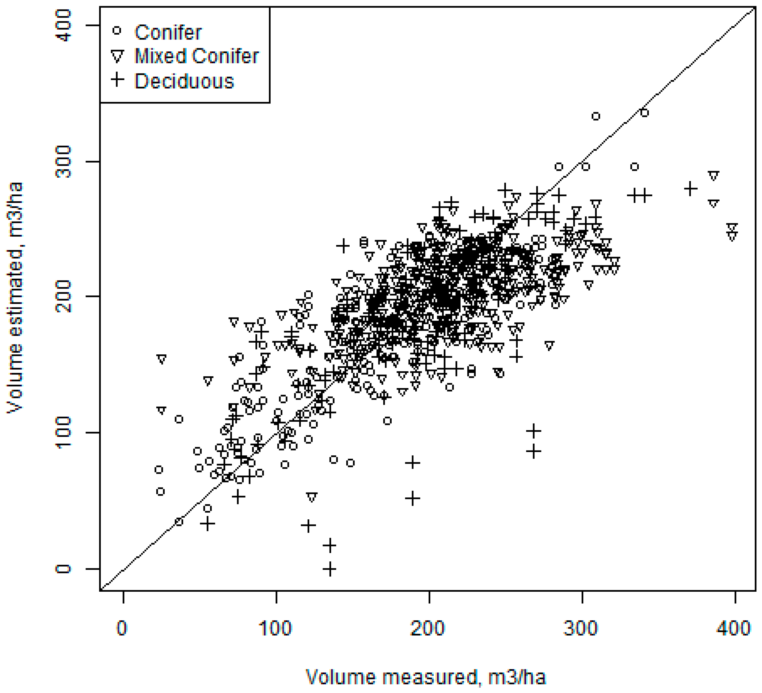
Coefficients of determination (R
2) for timber volume vary between 0.55–0.13, 0.65–0.012, and 0.53–0.22 for coniferous, deciduous, and mixed coniferous classes, respectively. The highest R
2 values were in the South area, with the highest number of field plots. The lowest values were in the mountainous East area. The scatter plot in
Figure 8 presents the measured field plot values against the estimated values in forest class-based estimation.
On the compartment level, the validation demonstrated smaller RMSE values than on the plot level (
Table 7).
The maximum likelihood classification of different land use classes resulted in an overall accuracy of 66.2% and a Kappa coefficient of 0.55, which indicates moderate agreement with ground truth classes (
Table 8). Classification results between forest and non-forest classes were slightly better, yielding an overall accuracy of 90.3% and a Kappa coefficient 0.66, which indicates a good agreement with ground truth classes. Results between three forest classes were 71.6% for overall accuracy and 0.56 for the Kappa coefficient, indicating moderate agreement with the ground truth.
4. Discussion
Satellite imagery-based forest inventories have been studied extensively and used for forest inventories all over the world for several decades. The camera relascope field measurement technique in turn has already been in use for some years as a forest inventory tool, e.g., at pre-harvesting inventory, measuring at specific forest compartments, and at other small- or medium-sized forest inventories [
42]. The concept of using a camera relascope for measuring field reference plots in satellite-based inventory was introduced few years ago (also [
16]). This research is unique in the sense that the data was acquired in a real operational large-scale forest inventory (ca. 2.6 million ha) conducted for industrial purposes. Also, it is the first study where camera relascope measurements based on automatic image interpretation are used in combination with satellite-based forest inventory.
Nevertheless, when it comes to similar studies in boreal forests, the results of such studies concerned with satellite imagery-based forest inventories over large areas have shown quite large variations in prediction accuracy, depending on the mean compartment size, study area, field reference data, and satellite data used. For example, [
43] achieved an RMSE of 36% at the compartment level when using national forest inventory field reference plots and medium-resolution satellite data with rather large average compartment sizes (19 ha) in Sweden. Ref [
44] reported a RMSE of 48% for the compartment-level total mean volume by using Landsat TM images with compartment-level field inventory data as the reference data in Finland. Ref [
45] used Landsat ETM+ and field sample plots in Alberta, Canada to estimate above-ground biomass and volume. The plot level RMSE in the modeling data was 40% when the volume was estimated using forest structural parameters (height and crown closure estimates), and 59% when direct estimation was used. The reported R
2 values, 0.71 and 0.30 for estimation through forest structural parameters and direct estimation, respectively, were significantly high [
45]. Unfortunately, compartment-level RMSEs were not reported. As [
46] points out in a discussion paper, the relative RMSE tends to decrease, when the reference area size increases. According to [
46], the RMSE of the total volume in satellite-based forest inventories has been between 40% and 60% at typical Finnish compartment levels (average compartment size 1–2 ha). More recent studies applying Sentinel-2 satellite images in the estimation of total volume have reported promising accuracies, although in small study areas. Research carried out in Norway in forest areas dominated by coniferous forests reported a relative RMSE of 30.1% and a R
2 of 0.48 when using field plots measured using traditional field methods [
47]. In the same study, training plots based on analyzing point cloud data from an unmanned aerial vehicle resulted in a relative RMSE of 37.5% and a R
2 of 0.30. The study was carried out in a small research area of 7330 ha, and field data comprised 33 plots of size 500 m
2. Similar results were reported in research done in Eastern Poland from a study area of 7800 ha dominated by Scots pine [
1]. Studies reported a relative RMSE for a volume of 35.1% and a R
2 of 0.24. The number of field plots were 94, and the size of the plot was 400 m
2. In that respect, the results of the present study, with RMSE being reported for both the plot level and the compartment level (with mean size of approximately 3 ha) in all major parts of the AOI (South, West and East) under 25%, have shown that they compare well to previous satellite-based forest inventories in coniferous forests of the boreal zone.
It is important to have a good spatial match between the field reference data and the corresponding satellite features. Ref [
45] presented a somewhat similar method to our study in improving the match between the field reference data and satellite image features. They used automatic segmentation to remove the spectrally uncharacteristic pixels from the 3 by 3 pixel window surrounding the field plot. In their case, the field plot size was only about half of the image pixel size. However, the segmentation improved the correlations between the image features, and the field measurements consistently compared with the full 3 by 3-pixel window. We used manual segmentation to delineate the plot and camera relascope to measure the sample plots. The camera relascope approach made it possible to measure larger reference plots, and not only one sample plot inside the segment, compared to manual field measurement methods with the given budget. However, it would have been interesting to compare the results between the manually measured smaller samples plot and camera relascope plots with the use of the segmentation method. This was unfortunately not possible, due to the budget limitations in our field campaign. Ref [
20] reported RMSEs of 19.7 to 29.7% for the plot level (plot size 32 by 32 m) basal area when comparing Trestima measurements with accurate manual field measurements. The most accurate results were achieved when the images were taken toward plot center. In [
20], the increase from four images per plot to eight images per plot improved the results only marginally. The mean diameter and height were measured more accurately: 5.2–11.6 and 10.0–13.6 for mean diameter and height, respectively, depending on the tree species [
20]. We measured larger plots in different conditions so that the results from [
20] are only directive for the measurement accuracy for our study.
Our results strengthen the findings of earlier studies concerning the suitability of camera relascope data in satellite-based forest inventory. Ref [
16] reported a RMSE of 29.7% for the basal area when comparing basal area measured with a Relasphone application and accurate field measurements in a small study area in Finland. The plot size in their data was between 0.2 and 1.0 ha, and on average, two Relasphone sample plots were measured in each plot. In the same study, the RMSE of the basal area in a test carried out in Durango, Mexico, was 17.2% and 18.0% for two observers. The reference plot size was 0.25 ha. Furthermore, the field plot data measured in Durango with a Relasphone was used as training data in a Landsat 8-based mean volume model. The standard error of the model estimate was 34% of the mean measured stem volumes [
16]. The reported RMSEs in [
16] cannot be used as a reference for the accuracy of our study; the Relasphone application uses a different sampling technique, and field plot size used was smaller. Despite the challenges in comparing the results of different studies, applying a camera relascope in measuring field training plots for satellite-based forest inventory seems to produce estimation accuracies that are comparable with methods applying manual field measurement methods for the same purpose, i.e., estimating the volume in boreal forests.
Applying multi-seasonal satellite data proved to be useful. Satellite features from Landsat 8 OLI images of both seasons were selected for almost every model. This indicates that multi-seasonal satellite images have more information than the imagery from one season in the context of the forest inventory. Thus, when applicable, it is recommended to search for multi-seasonal imagery, and to test case-by-case if leaf-on, leaf-off or a combination of these produced the best results.
The presented concept and methodology was very promising for being used in large areas of satellite-based forest inventory and mapping projects. Future research and testing were still needed to validate the methodology against other field measurement techniques, and to fine tune the optimal plot type and image sample design. Also, the applicability in more challenging environments with more heterogenous forest structures and a wider variety of species should be tested.

 and
and 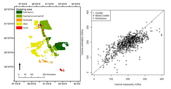


