Article

Canopy Effects on Snow Accumulation: Observations from Lidar, Canonical-View Photos, and Continuous Ground Measurements from Sensor Networks

1
Department of Civil and Environmental Engineering, University of California, Berkeley, CA 94720, USA
2
Sierra Nevada Research Institute, University of California, Merced, CA 95343, USA
3
Department of Civil and Environmental Engineering, University of Texas, Austin, TX 78712, USA
*
Author to whom correspondence should be addressed.
Remote Sens. 2018, 10(11), 1769; https://doi.org/10.3390/rs10111769
Submission received: 14 August 2018 / Revised: 18 October 2018 / Accepted: 30 October 2018 / Published: 8 November 2018
(This article belongs to the Special Issue Remote Sensing in Forest Hydrology)

Abstract

:
A variety of canopy metrics were extracted from the snow-off airborne light detection and ranging (lidar) measurements over three study areas in the central and southern Sierra Nevada. Two of the sites, Providence and Wolverton, had wireless snow-depth sensors since 2008, with the third site, Pinecrest having sensors since 2014. At Wolverton and Pinecrest, images were captured and the sky-view factors were derived from hemispherical-view photos. We found the variation of snow accumulation across the landscape to be significantly related to canopy-cover conditions. Using a regularized regression model Elastic Net to model the normalized snow accumulation with canopy metrics as independent variables, we found that about 50 % of snow accumulation variability at each site can be explained by the canopy metrics from lidar.

Graphical Abstract

1. Introduction

The snowpack in California’s Sierra Nevada has long served as the primary water resource for agricultural and urban uses [1]. For seasonal forecasts following the onset of snow melt, the estimation methods are turning from statistical estimates that use historical records to spatio-temporal water-balance estimates with integrated time series and spatial data [2,3]. Quantifying the spatio-temporal distribution of snow accumulation enables more-accurate forecasts of snow melt and streamflow, especially in a warming climate as statistical relations broke down; and it is also a long-standing challenge in snow hydrology [4,5]. In the high Sierra, orographic effects drive solid-phase precipitation falling over mid-to-high elevations [6,7]. During the snow-accumulation period, vegetation intercepts snowfall, causing the snowpack to distribute unevenly under the canopy. In boreal forests, as much as 60% of cumulative snowfall may be intercepted by forest canopy in mid-winter, and annual sublimation losses can be 30–40% of annual snowfall [8,9]. In mixed-conifer forest, both observations and modeling results have shown that canopies can reduce 10–25% of total snow accumulation in surrounding open areas; and the reduction can be 30–40% for snow accumulation under canopy [10]. The canopy effects are also found to vary with local landscapes [11]. Accurately quantifying canopy interception of snowfall is the foundation to estimate the total accumulation and snow melt with higher accuracy and precision during the spring season.
The canopy interception of snowfall can be quantified as the snow-storage capacity of the canopy and interception efficiency (interception/snowfall). The snow-storage capacity is the maximum amount of snowfall that can be intercepted by the canopy. It is determined by the leaf area, tree species, and initial canopy snow load [12]. The interception efficiency is found to decrease with increasing snowfall, initial canopy snow load and temperature. It has been observed to increase with leaf-area index (LAI) and canopy coverage [8,13].
The coniferous canopies interception of snowfall is challenging to directly measure and quantify, which has led to interception being inferred from snowfall patterns on the ground, as noted above. Previous studies designed special weighing devices such that the weight of the intercepted snow and accumulated snow can be measured at the same time. The total snow interception is found to be correlated with the season or event snowfall [8,12]. Similar findings were observed from simulating the snow evolution by using energy balance models with canopy metrics [14,15,16]. Thus, several process models have incorporated this statistical finding to estimate canopy-cover effects on snow accumulation [17,18,19,20].
A common approach to calculate canopy interception uses canopy metrics that are highly correlated with snow accumulation. Retrieving canopy metrics has advanced in recent years. The technology has been advancing from the traditional plant-canopy analyzer [18,21,22,23,24], to hemispherical-view camera [25,26], and recently, to lidar [27,28]. The plant canopy analyzer was commonly used for retrieving the LAI in the forest. By using the hemispherical-view camera, the pixels of an image can be classified as either canopy-covered or clear; and thus the percentage of clear view for each zenith angle can be quantified as the sky-view factor, which was also found to be a statistically significant predictors for parameterizing snowfall interception in process models [25,29]. The point-cloud data collected using lidar can be used for reconstructing the 3-dimensional canopy structures if the point-cloud is sufficiently dense. Algorithms have been developed for deriving LAI from lidar point clouds, and additional canopy metrics from lidar often get derived for quantifying the snowfall interception [30].
In addition to canopy-metric retrieval from lidar, canopy effects can also be quantified using statistical models, with dense spatial measurements of snow depth or snow water equivalent (SWE) [28,29]. Most previous studies were conducted using lidar measurements, either airborne or terrestrial. Both the airborne and terrestrial lidar can provide dense spatial snow-depth measurements (>10 pts / m ). With the extensive footprint provided by airborne lidar scans, the canopy effect on snowpack spatial distribution can be quantified with large samples. Terrestrial lidar has a much smaller footprint compared to airborne lidar [31], however, it is able to provide multiple scans per season. Thus the temporal variation in canopy effects can also be determined.
One short coming in using lidar is that it can lack temporal completeness, especially during the precipitation season, when cloud cover limits taking measurements. Lidar also requires clear-sky conditions to take measurements to prevent the laser pulse intensity from attenuating because of rain drops and snow flakes [32]. A dense cluster of snow-depth sensors can compensate the weakness of lidar in terms of temporal consistency. Combining the vegetation structures derived from lidar measurements and continuous snow-depth measurements, there is potential for the spatial variation of snow accumulation to be accurately quantified. In our study, we used long-term spatially dense snow measurements in the Sierra Nevada, together with the lidar-derived canopy metrics, to study the canopy effect on seasonal snow accumulation.
The overall aim of the work reported here is to explain and predict the spatial variability of snow accumulation using lidar-derived canopy metrics and clustered snow-depth sensor measurements. We address two major question. First, to what extent can one use lidar-derived canopy metrics to predict the snow accumulation spatially? Second, what is the relative importance of various lidar-derived canopy metrics?

2. Methods

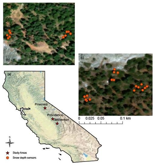
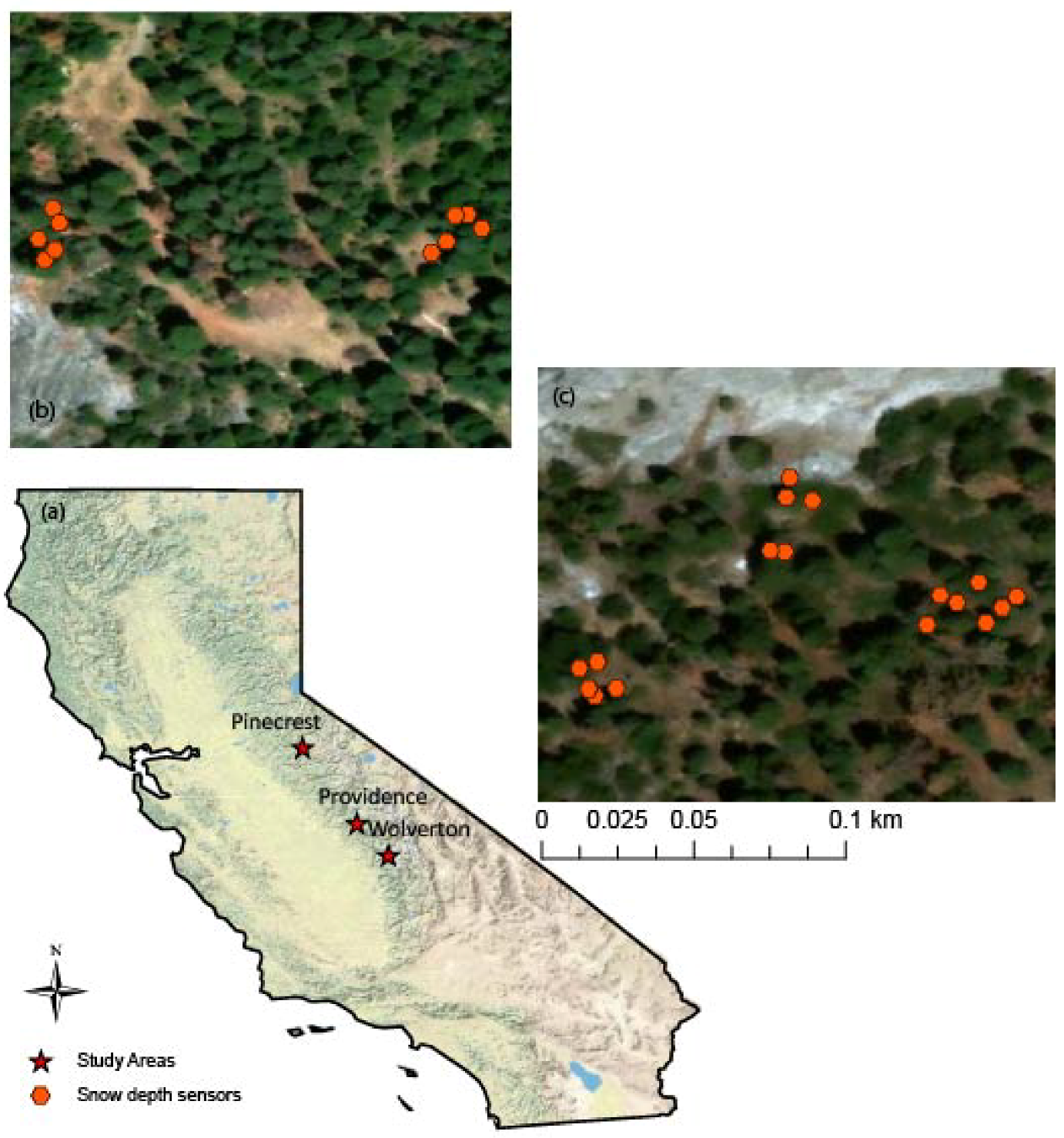
2.1. Study Areas and Snow-Depth Sensor Data

The study was conducted over three areas in California’s central and southern Sierra Nevada (Figure 1a). For each study area, snow-depth sensors (Judd Communications) were deployed in clusters (Figure 1b,c; Table 1), with topographic characteristics (elevation, aspect) varying between clusters and canopy-cover conditions varying within each cluster. The snow-depth sensors have an accuracy of ±1 cm , with measurement range of 0.5 to 10 m and beam width of 22 degrees. All study sites encounter wet winter for most of the years because of their proximity to the Pacific. Due to the orographic effect, most precipitation falls as rain at elevations below 1500 m and as snow above 2000 m [28]. The date of peak snow-accumulation is commonly recognized as 1 April [1]. Pinecrest, located in the Stanislaus-Tuolumne Experimental Forest, is the lowest in elevation and is also relatively flat. The lower site of Providence has a similar elevation range as Pinecrest, and the upper site is 200 m higher. Wolverton, the highest of the three study areas, receives mainly snow, whereas Providence and Pinecrest receive precipitation as both rain and snow. There were 12 sensors installed at Pinecrest in 2014, 27 sensors at Providence, and 25 sensors at Wolverton, installed in 2008. All time-series data are shown in Figure S1.

2.2. Lidar Data

The lidar survey was performed in August 2010. The flight parameters and sensor settings are described in Table 2. The point-cloud lidar data were used for generating raster data sets. The raw point-cloud files, we divided them into 250 × 250-m tiles using LAStools lidar-processing software [33]. For all data points in the point-cloud data set, each one of them has a classification attribute and the data point was a laser return from the ground if the classification attribute equals 2. We extracted the ground points from each tile and interpolated them into a 0.5-m resolution digital elevation model (DEM) using a simple kriging model with a spherical covariance function [34]. The 250 × 250-m DEM tiles were mosaic-ed together to form a single DEM of the study area. A digital surface model (DSM) was generated from all first returns of the lidar point cloud. Subtracting the DEM from the DSM produces the canopy-height model (CHM). Individual trees were segmented out from the CHM using a watershed-segmentation algorithm implemented in SAGA GIS software [35]. The segmentation was conducted after applying a Gaussian filter with a 3 × 3 moving window to fill pits in CHM and suppress irrelevant local maximas [36,37]. Over each snow sensor location, canopy metrics, including mean canopy height, standard deviation of canopy height, and canopy-cover fractions, were extracted at search radii from 2 to 40 m at 1-m increments. These canopy metrics were calculated by masking out the circular area with certain radius around the snow-depth sensor location. The canopy-height statistics were calculated with the CHM pixels that are within the circular area. The canopy-cover fractions were determined by calculating the percentage of canopy pixels within the circular area. The canopy pixel is classified from the CHM if a pixel value is greater than 2 m [28]. The distance from the sensor location to the closest tree trunk was also calculated by using the segmented-tree information. In total we derived more than 100 canopy metrics from the above methods.

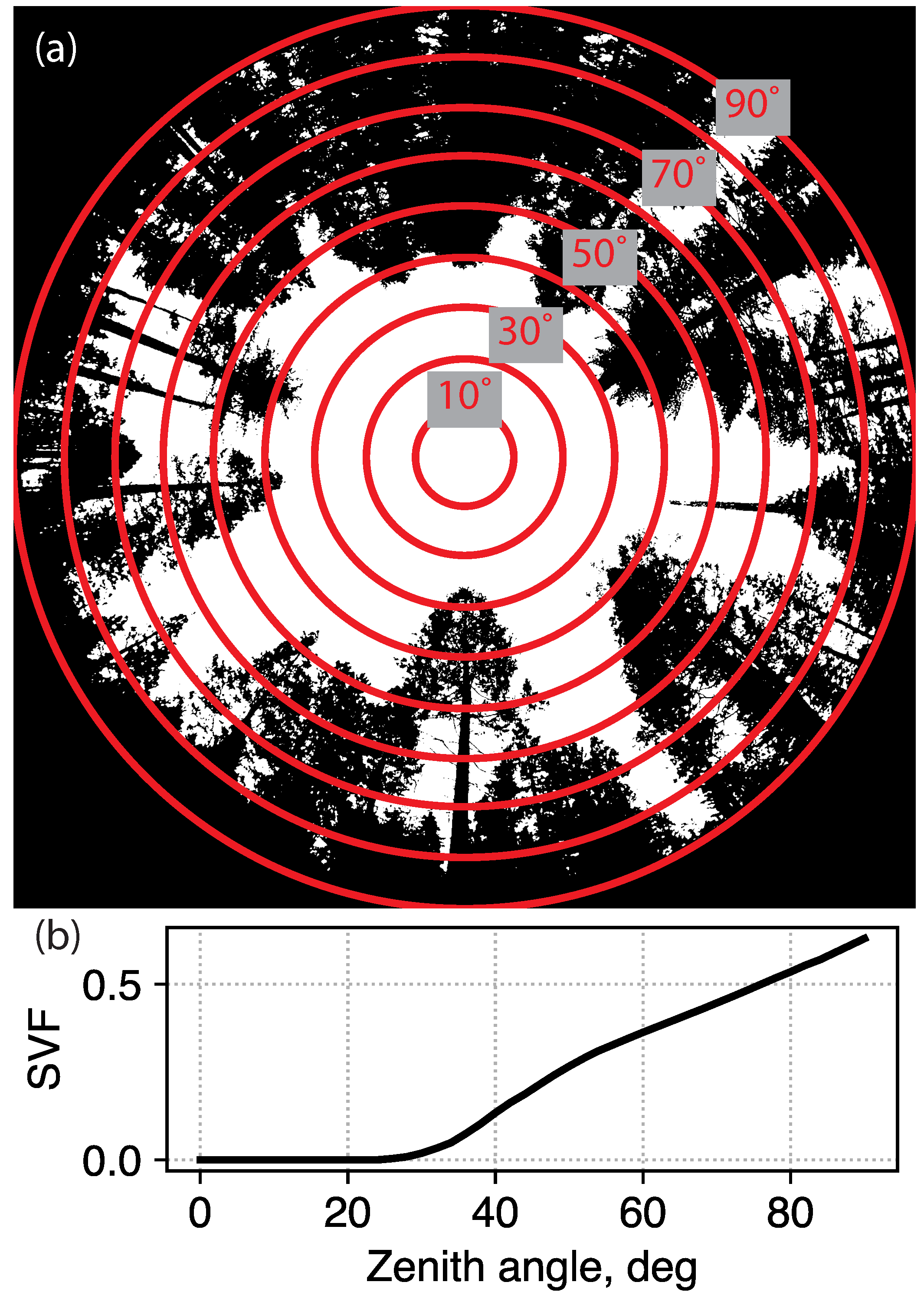
2.3. Canonical-View Images

The canonical-view images, are the hemispherical photos taken at each snow-depth sensor. The sky-view factors (f, SVF) at each individual zenith angle θ were derived from the raw image, with each pixel classified into binary representation of sky and non-sky elements. Within each zenith angle, the SVF was estimated by the ratio of the number of sky pixels and the number of total pixels. An example of the canonical-view image and the estimated SVF is shown in Figure 2. The total sky-view factor at each sensor node was also estimated using the equation below [29,38],
f t o t = θ = 1 θ = 90 sin ( θ ) f ( θ ) θ = 1 θ = 90 sin ( θ )
The sky-view-factor data are available for Wolverton and Pinecrest. Considering that only 6 sensor locations at Pinecrest have the images, the data available are not enough to build robust statistical models, so Pinecrest is not included in analysis with the sky-view factors. We included the total sky-view factor and the sky-view factors at each zenith angle as independent variables for modeling the snow accumulation observed at each sensor location. The results are compared with the modeled results that use lidar-derived canopy metrics as predictors.

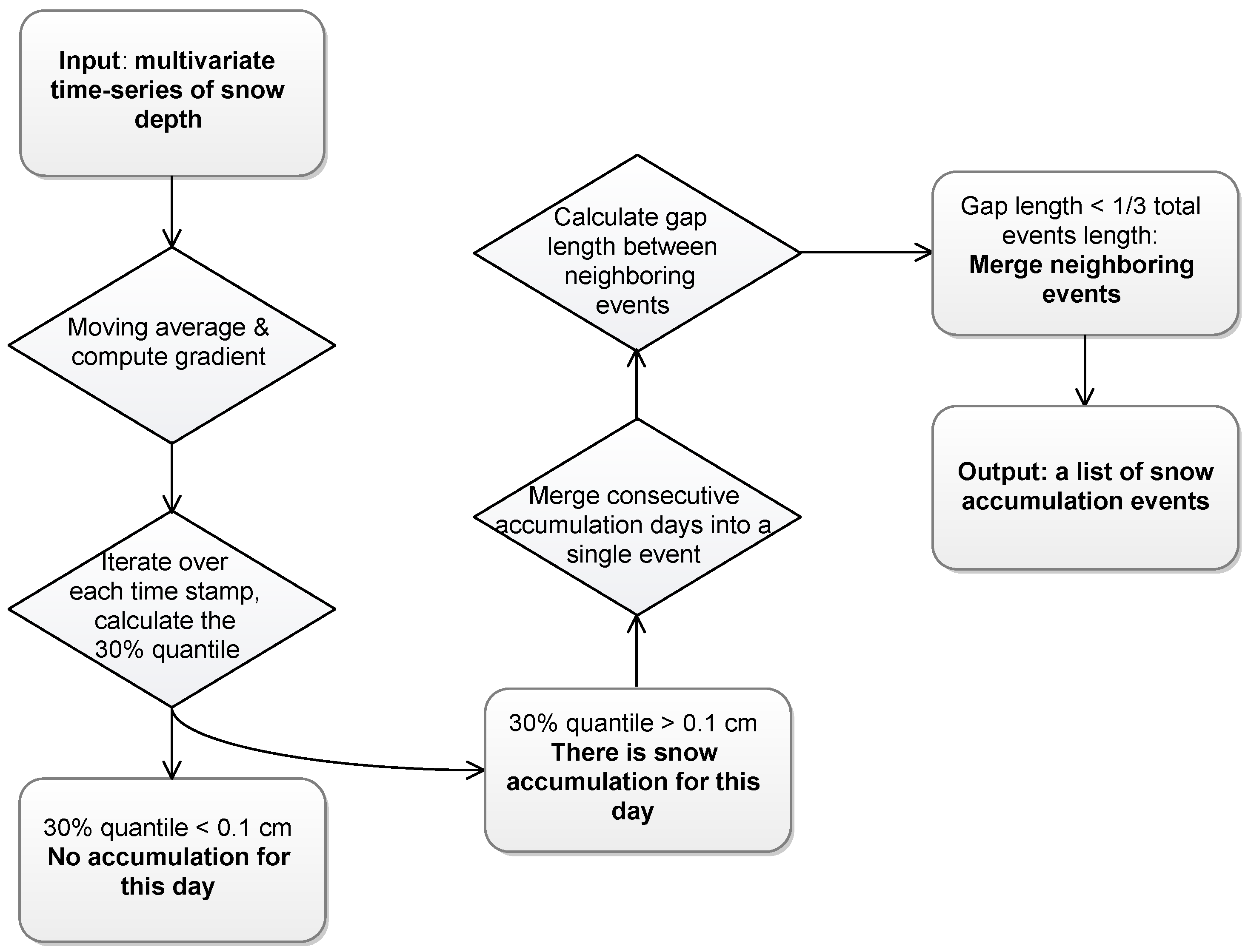
2.4. Snow Accumulation Events Detection

The data availability over time for each site is shown in Table 1. We studied the canopy effect on snow accumulation using the following procedure (Figure 3).
  • Get the moving average of each snow-depth time series with a window size of 2 days. Then calculate the 1st order gradient of the time series. This made estimates less vulnerable to high-frequency noise in the snow-depth data.
  • The 1st-order gradients over all sensors, were used to calculate the x % quantile of the gradient. The quantile statistic was then compared with a pre-configured threshold to determine if most sensors observed snow accumulation. Neighboring accumulating days were then grouped together to form a single event.
  • For snow-accumulation event detection, we set the quantile for snow accumulation as 30%. It means that if 30% of sensors show an ascending trend in one day, we can classify this day as an accumulation day.
  • The daily gradient thresholds were also need to be optimized, along with the gap length between two adjacent snow accumulation dates. The optimized threshold for snow accumulation events is 0.1 cm. If two snow accumulation events were temporally close, we used the following rule to determine if the two neighboring events can be merged together or not.
For snow-accumulation events, the optimized way to combine two neighboring events is to first judge if the length of gaps between two events are shorter than one third of the sum of length of two events. Then, if the snow depth data for most sensors does not show a descending trend during the gap period, the two close events were combined into one.
The parameters that were used in the above steps were derived from a sensitivity analysis. The analysis was performed based on the snow-depth time series collected from Wolverton in water year 2010. We manually extracted the snow-accumulation periods from the multivariate time-series data and used the extracted periods as the standard to be compared with. The analysis was conducted in a Monte Carlo manner, with parameters randomly drawn from their predefined sets. The algorithm classifies each day of the water year as either an accumulation day or non-accumulation day. Comparing the results produced from the algorithm to the manually extracted periods, we calculated precision and recall as the classification accuracy for the entire year. We used these two metrics to determine the near-optimal parameter set that was used.

2.5. Statistical Analysis

All extracted accumulation events were used for statistical modeling, with features derived from the lidar data and the sky-view factors derived from the canonical-view camera images. We conducted regression analysis to study if canopy metrics can be used as predictors for estimating snow accumulation at various canopy-covered conditions. For each individual accumulation event, the total snow accumulation at each sensor node was estimated as Δ H = H k H 0 where H k is the snow-depth at the last time step and H 0 is the snow depth when the precipitation event started. Considering topographic effects on precipitation along the elevation gradient, we offset the total solid precipitation for each individual event at each site using elevation. For all study sites, the sensors were clustered in a lower-elevation site and a upper-elevation site. We calculated the mean snow accumulation at both clusters and we subtracted the absolute difference of the two averages from the snow accumulations at the upper site to derive the offset accumulations. The offset results were standardized to the range of 0–1. The detrended target values are regressed using Elastic Net (implemented in Python Scikit-Learn [39]), which is a regularized regression method that linearly combines both L 1 and L 2 penalties in the regression model. We assumed a linear regression problem defined as:
y = X β + ε
where y is the target value and X is the matrix of all covariates. The regression coefficient β ^ can be estimated with:
β ^ = arg min β ( y X β 2 + λ 2 β 2 + λ 1 β 1 )
where λ 1 and λ 2 are the weightings for the L 1 and L 2 regularizations, respectively. The Elastic Net was chosen over other regularized regression approaches for its ability to address correlated covariates and high numbers of covariates [40,41]. We have also considered nonlinear and ensemble models, such as the Random Forest regression, but the performance was not as good as the Elastic Net regression (results not shown). In our case, the canopy metrics can be highly correlated when the search radii are close and the number of covariates included in our analysis is more than 100.
In order to have representative estimates of how much variability can be explained by the Elastic Net model we used bootstrap to resample the data for 20 iterations and estimated the cross-validated coefficient of determination ( R 2 ) within each iteration. The distribution of the R 2 was estimated from multiple bootstrapping results.
We also applied correlation analysis to explore the most-informative radius of lidar-derived canopy features and the most-informative zenith angle of the sky-view factors from the canonical view images. We computed the correlation between the snow accumulation from each individual event and the lidar-derived mean canopy height at various search radii and at various zenith angles. The correlation coefficients (R) were compared at various radii and angles to select the optimal radius and zenith angle. Considering that Pinecrest has a relatively short record, most of which is during a recent drought, we did not conduct the analysis for Pinecrest. Also, camera images are not available for Providence, thus we only conducted radius dependency analysis at that site. At Wolverton, we selected a few near-optimal searching radii and zenith angles. We used these selected variables and conducted a step-wise linear regression with forward selection [42] for exploring the relative importance between variables. We used step-wise linear regression rather than other embedded feature selection approaches in order to show the results from s perspective of correlations.

3. Results

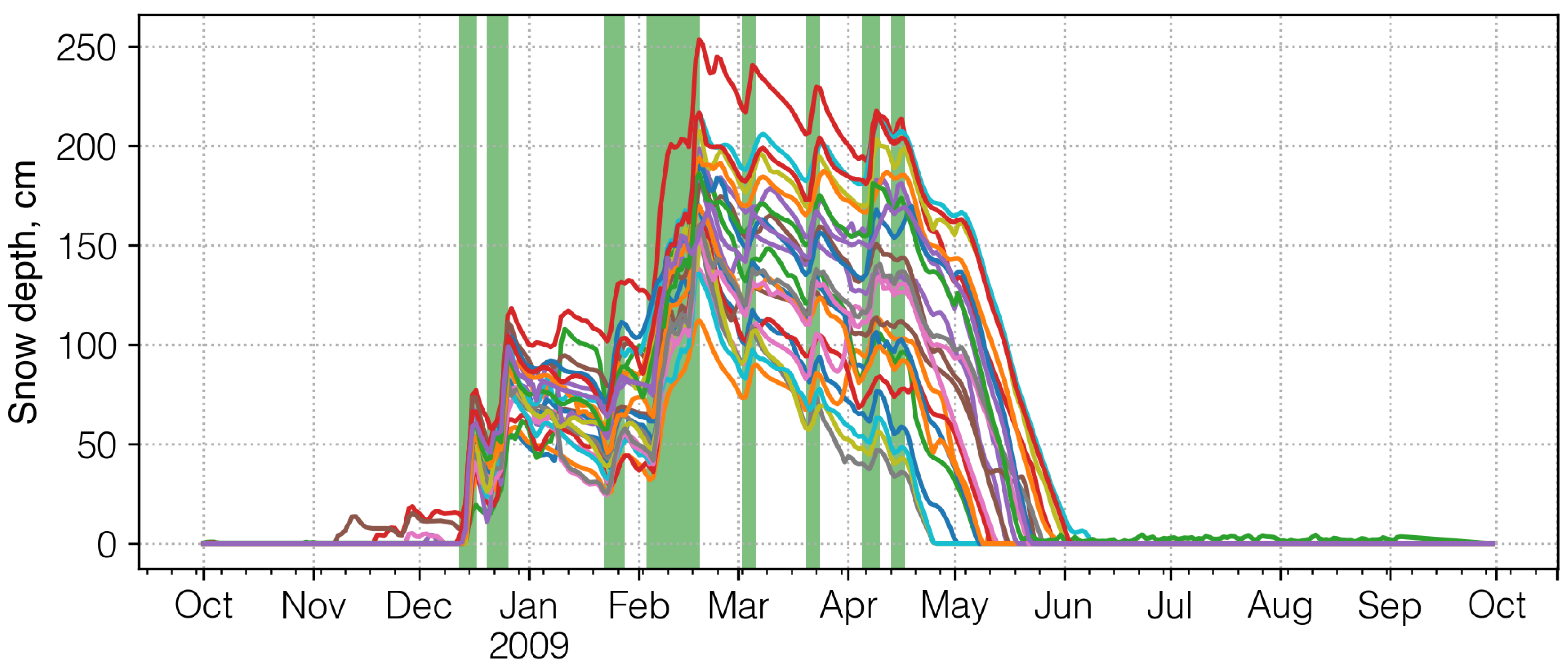
3.1. Snow Accumulation Events Extracted from Snow-Depth Time Series

Before running the snow-accumulation detection algorithm on all time series, we performed a sensitivity analysis on the 2010 time-series data from Wolverton. We found that as long as the gap length is about 1 / 3 of the total length of the neighboring events, with the snow-accumulation rate threshold being more than 0.1 cm and less than 1 cm, and the quantile of the snow-accumulation sensors being in between 30% to 50%, both precision and recall are higher than other parameter sets (see Figure S2 for analysis results.)
We applied our snow-accumulation events-extraction algorithm on all snow-depth sensors for all time periods when cleaned snow-depth data were available. The performance of the detection algorithm is similar to manual extraction, done previously for some years (data not shown). As shown in Figure 4, the algorithm is able to detect most major snow-accumulation periods. A summary of accumulation events for each site is shown in Table S1 and the distribution of the magnitude of the accumulation at each study area is shown in Figure S3. Wolverton has more events because it is at higher elevations. At the time of this analysis, 2016–17 data were not available for Wolverton.

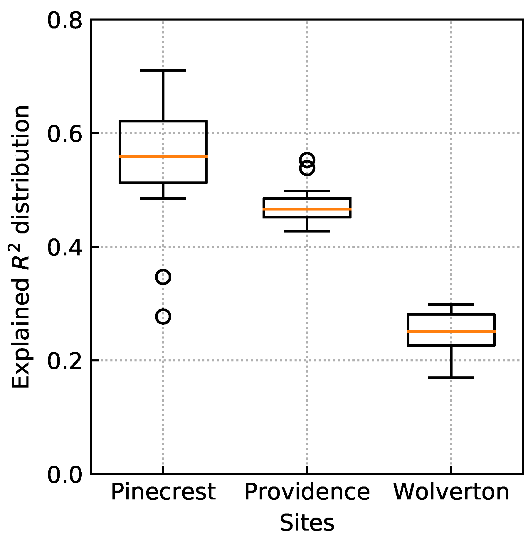
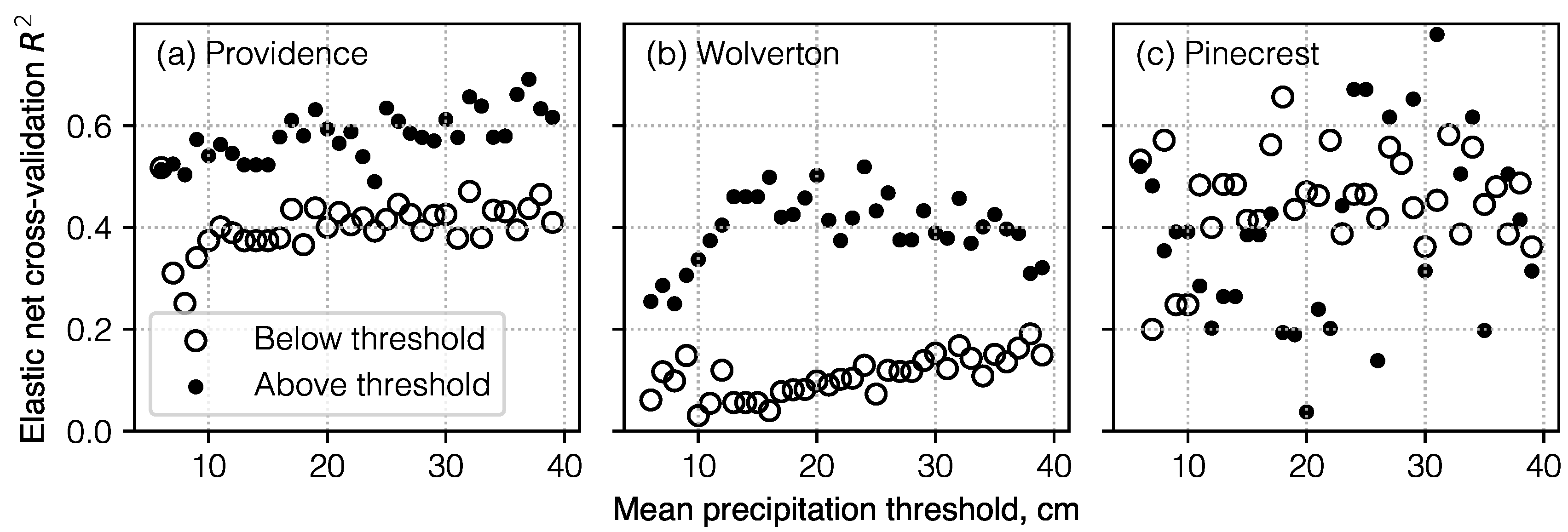
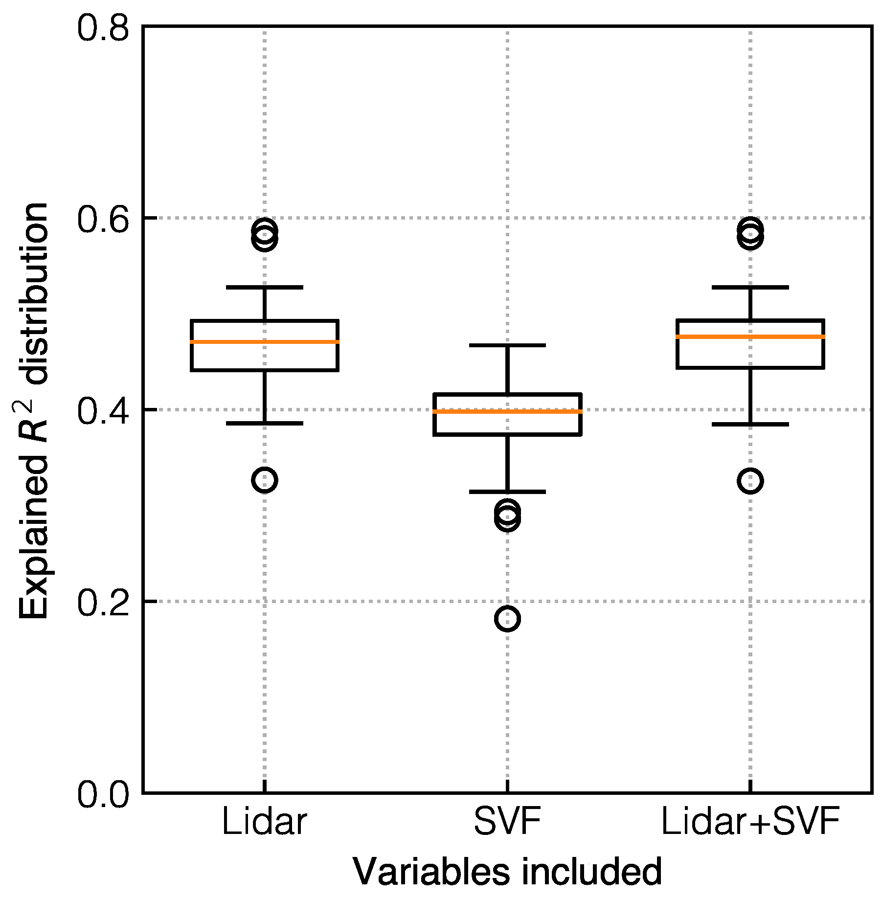
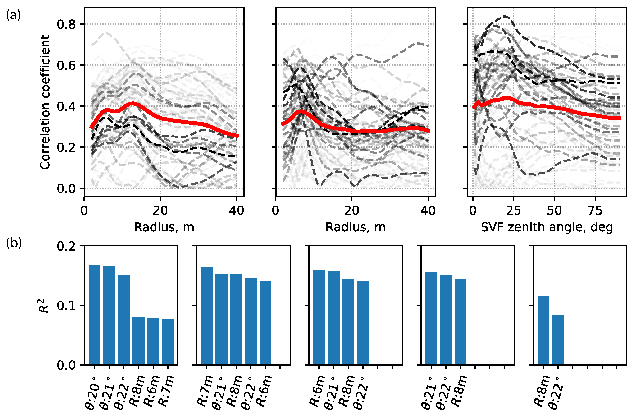
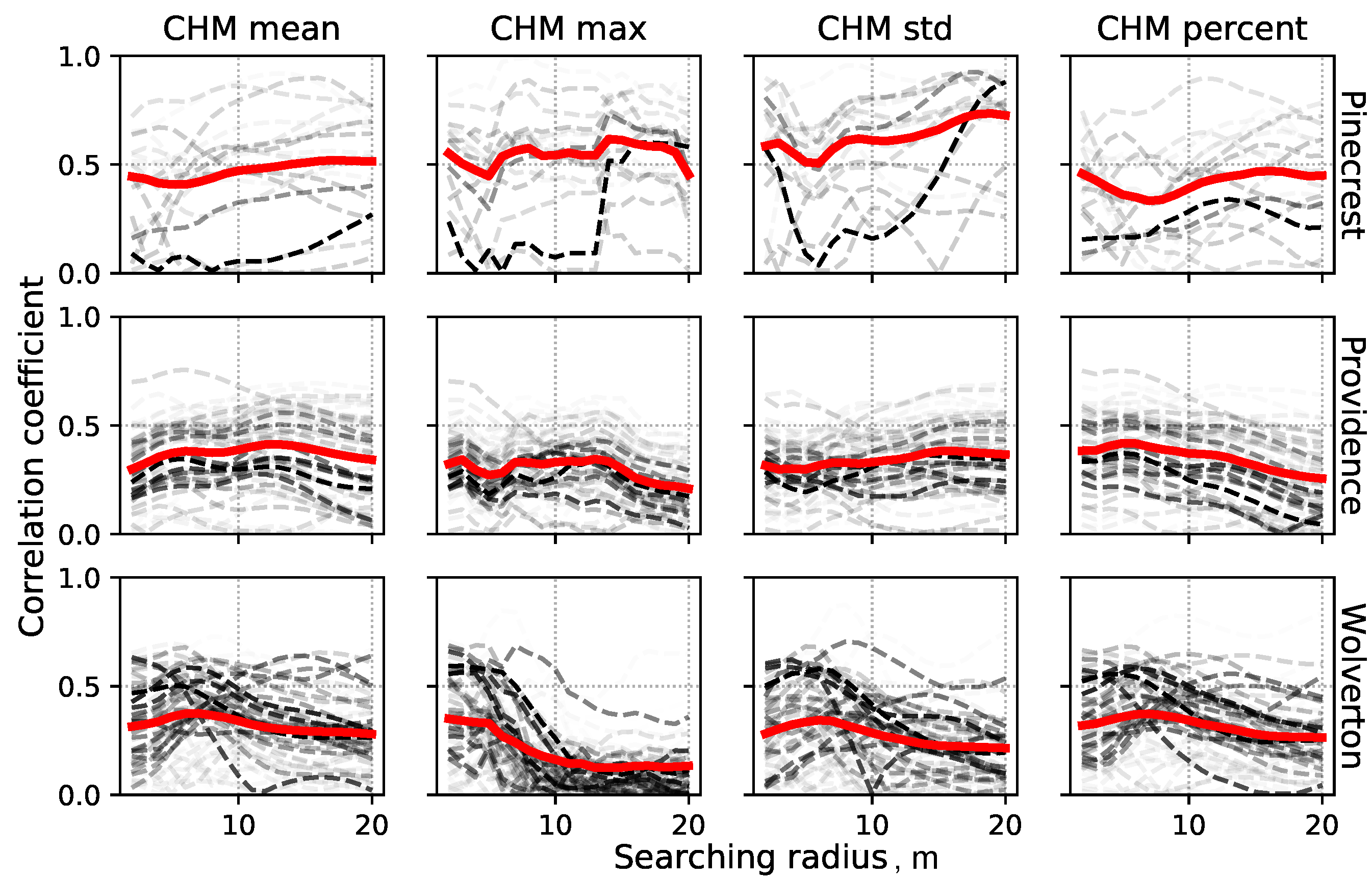
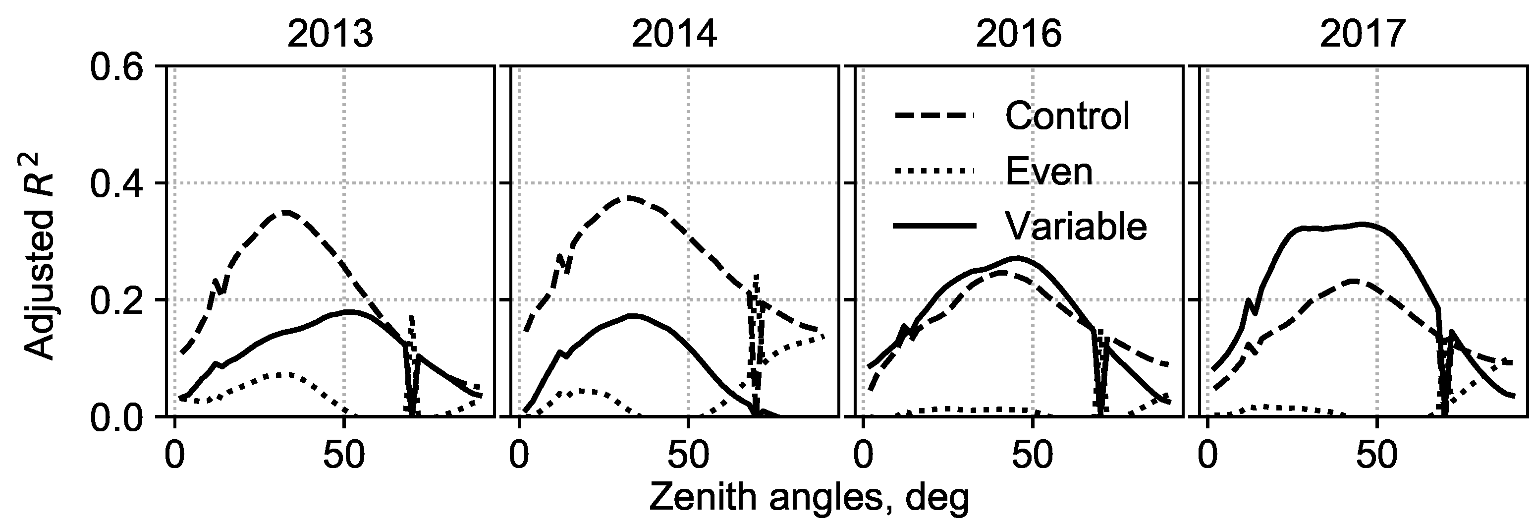
3.2. Statistical Modeling Results

The variability that the Elastic Net model can explain over the three sites is shown as in Figure 5. The uncertainty range of the variability that can be explained by the Elastic Net model is much larger for the Pinecrest (0.55 on average and ± 0.1 of variation) analysis than the other two areas (0.45 on average at Providence and 0.25 on average at Wolverton, and ± 0.05 of variation for both). Note that Pinecrest is the lowest and Wolverton the highest elevation of the 3 sites.
At Providence and Wolverton, excluding the minor accumulation events (≤15 cm) can increase the variability that can be explained by the Elastic Net model, with more than 50% explained at Providence and 40–50% explained at Wolverton (Figure 6a,b). Due to the fact that for minor accumulation events the signal strengths are not greater than the uncertainty range of the snow-depth sensors, including these data points will degrade the performance of the Elastic Net model. At Wolverton, the spatial variability of snow accumulation that can be explained reaches the maximum when the mean snow accumulation is between 15 cm and 30 cm (Figure 6b). At Pinecrest, no particular trends can be observed, as the number of data points is limited. When including most of the data points, the variability explained stabilized around 40–60% (Figure 6c).
For Wolverton, the only study area that both SVF and lidar are available, the trends in Figure 6b show that R 2 is the maximum when the threshold is above 15 cm. We thus filtered the data with mean precipitation that are below 15 cm. We conducted three sets of analysis, including using lidar-derived canopy metrics as the predictors, using SVF as the predictors, and using both lidar and SVF as the predictors in the Elastic Net model. As shown in Figure 7, the coefficient of determination calculated from 20 bootstrapping runs of predicting the snow accumulation suggests that the trained models are more accurate in predicting the total snow accumulation at the unobserved sensor locations if using lidar-derived variables because the variability of the R 2 is larger than that using sky-view factor. Also, the third box-plot of this figure suggests that using both lidar-derived variables and sky-view factors is only as good as just using lidar, indicating that the sky-view factors do not provide more information than lidar in terms of predicting snow accumulation.
The canopy-related variables derived from lidar and canonical-view images are compared based on the correlation coefficients between the total solid precipitation and the canopy attributes over each individual event across sensors, as well as the step-wise linear regression. The correlation analysis (Figure 8a) shows that the surrounding canopies have a stronger effect on the snow accumulation on the ground than does the canopy right above. The canopy mean height within a 15-m radius at Providence is the most effective distance, while the optimal radius is about 8 m at Wolverton. For sky-view factor, the optimal zenith angle is about 21 ° at Wolverton. In Figure 8a, we identify each individual precipitation event by the transparency of each curve, from which we can see that heavier storms have more dominant weights for characterizing the canopy effects at different search radii from lidar data and zenith angles from canonical-view photos. In addition, the step-wise regression analysis (Figure 8b) conducted on the selected optimal variables of lidar-derived and canonical-view imagery features suggest that the canonical-view imagery features are more important and the marginal information that lidar provides is limited comparing to the first canonical-view imagery feature selected.
The canopy-cover information is slightly more important than canopy-height metrics, which include tree heights and tree-height standard deviations. This was verified by correlation coefficients in the regression analysis between snow accumulation and both tree height at incremental search radii and SVF at incremental zenith angles. In general, SVFs are more correlated with snow accumulation than is tree height. The step-wise regression analysis also suggests that the sky-view factor at the optimal zenith angle, is more important than is tree height at the optimal search radius. Although the tree height is an important metric characterizing trees in the forest, it does not necessarily represent the density and interception capacity of the canopy. Even though sky-view factor only represents the canopy-cover condition at the lowest layer of canopy, it is still a direct index representing the interception capacity of part of the tree crown. In contrast, the tree height does not necessarily represent the interception capacity, which is the reason that the lidar-derived variables are not as important as the sky-view factors. Please note that having a few important variables does not guarantee more-accurate estimates in snow accumulation. Combining all lidar-derived variables together, we have made more-accurate estimates of snow accumulation than using the sky-view factors (Figure 7).
In addition, we compared the correlation coefficient between different types of lidar-derived canopy-related features and the snow accumulation over different sensor nodes. The features include mean canopy height over the search radii, standard deviation of the height, maximum canopy height, and canopy coverage. As is shown in Figure 9, the amount of data at Pinecrest is not enough to draw solid conclusions. At Providence and Wolverton the correlation coefficient is a concave shaped function of both canopy-height mean and canopy coverage at various searching radii. The maximum canopy height at the smallest search radius correlates the most with the snow accumulation. The standard deviations of the canopy heights at various search radii show contrast trends at Providence and Wolverton.

4. Discussion

4.1. Canopy Effect at Different Elevations

Among the three sites studied, the variability of snow accumulation that the canopy-related variables can explain varies from site to site and also depends on the mean cumulative precipitation over the entire event. The difference between sites can be attributed to different elevations, as the canopy-cover density decreases as elevation increases and the solid-phase precipitation increases with elevation. For example, the instrumentation locations at Pinecrest and Providence are at much lower elevations compared to Wolverton. About 40% of snow-accumulation variability is attributable to the canopy effects at these two sites, however only 25% can be explained over Wolverton. This suggests that at higher elevations, where precipitations is heavier, the canopy effects can be diluted by the heavy snowfall, which is similar to previous findings [13], where total interception of snowfall saturated when the total precipitation reached certain thresholds for different tree species. In addition, we observed some noise introduced by the low-precipitation events in the regression analysis [11]. Figure 6 suggests that the spatial variability of precipitation is less explainable by the canopy-related variables when the total precipitation is small.
The difference of the canopy effect on snow accumulation at the lower elevations is also affected by the rain-on-snow events. Analyzing rain-on-snow events would need more meteorological data, especially temperature and relative humidity, for estimating the rain-snow partition along the elevation gradient [43]. A rain event can accelerate snowmelt by altering the energy balance of the snowpack [44,45]. As such, the snow accumulation during mixed rain and snow events reflects the net of snow precipitation and snowmelt. The spatial patterns of total snow accumulation at each location need to be analyzed with a full surface-energy-balance model such that canopy effects on accumulations can be described.

4.2. Forest Thinning Effects on Snow Accumulations

At Pinecrest, considering that not all sensor locations have sky-view factors, we used multi-year snow-depth data from surveys and the sky-view factors for all survey locations, comparing correlation patterns observed from this site with Wolverton. Similar to Figure 8a, in Figure 10 we see that the adjusted R 2 peaked around a zenith angle of 30 ° . Over the snow survey locations, the forest above has been thinned the same amount, but with either even density or heterogeneous density. It seems that even thinning has a greater impact on canopy effects, as the correlation coefficient is close to zero for most zenith angles except when the angle approaches 90 degrees. The thinning with variable forest density holds a similar pattern comparing to the control group, with adjusted R 2 peaked around a zenith angle of 30– 50 ° . But the magnitudes of correlations are smaller during the dry years (2013–2014).
Comparing lidar-derived canopy metrics at increment radii, Figure 9 suggests that the most important canopy structures may not be the canopy layers right above the measured locations. The canopy surrounding within a few meters could be even more important, as the interception capacity can be larger when the trees are clustered together versus for a single tree. Our findings are aligned with what was found previously [11,12]: multi-layered forest cover increases canopy-interception efficiency, resulting in significant reductions in subcanopy snow accumulation. Even thinning will make the trees evenly spaced [46], and as such the number of forest layers will be greatly reduced, with commensurate reduction in canopy interception of snow. This is the reason that the snow depth is not correlated with the SVF at any zenith angles in the evenly thinned forest at Pinecrest, while the control group and the forest with variable density still retain multi-layered canopies.

4.3. Potentials to Extend the Analysis

The integrated sensing system, including lidar, canonical-view images, and ground measurements, allowed us to study canopy effects on snow accumulations. The snow-accumulation detection algorithm can be applied to most mountainous areas that have seasonal snow, with minor tuning of parameters to fit the local snow-accumulation patterns. However, the current statistical analysis is limited to only canopy effects, and did not address the interactions between canopy and terrain or canopy and meteorological conditions. Although the current statistical model trained with canopy metrics can explain about 50% of the snow-accumulation variability, more may be explained when local topography and meteorology are considered. For canopy-terrain interactions, a spatially denser deployment of snow-depth sensors is needed in order to build relationships between terrain and snow that are statistically significant. For meteorological data, other than air temperature and relative humidity mentioned in Section 4.1, wind distribution is also important as it affects canopy interception, snow unloading from the canopy, and snow redistribution in the forest [8,12]. We did not include wind in our analysis, as there is limited wind monitoring on site and the wind effect is negligible in the Sierra Nevada [30], but wind can be important for regions like the Alps and the Rocky Mountains.

5. Conclusions

We found correlations between the lidar-derived canopy attributes and snow accumulation extracted from the multi-year time-series snow-depth measurements. The correlation is stronger when the precipitation event has more than 15 cm of snow accumulation. And the correlation is also much stronger at a lower elevation (<2000 m) because of denser vegetation. Although the lidar-derived canopy attributes are complementary to sky-view factors in explaining the snow-accumulation variability, the sky-view factors at certain zenith angles are more important than lidar-derived variables in terms of correlation. According to the correlation analysis using lidar-derived canopy metrics at various search radii, the canopy surrounding the snow surface within 8-m radius is more important than canopy structures within either smaller radius or larger radius, indicating that a clustered canopy effect is stronger than is canopy of a single tree. The above findings suggest great potential of using lidar and ground measurements for studying canopy effects on mountain snowpack.

Author Contributions

Z.Z. designed research, performed data analysis, and wrote the paper. Q.M. performed lidar data processing. K.Q. developed the snow accumulation detection algorithm. R.C.B. helped with designing the research and writing the paper.

Funding

The work presented in this paper is supported by the UC Office of the President’s Multi-Campus Research Programs and Initiatives (MR-15-328473) through the UC Water Security and Sustainability Research Initiative (grant No. 13941).

Acknowledgments

We acknowledge the National Science Foundation (NSF) through the Southern Sierra Critical Zone Observatory (NSF Award Numbers 1331939 and 1239521). The portion of the work conducted at Pinecrest was supported in part by the USDA, National Institute of Food and Agriculture (NIFA) program, grant number 11-03859.

Conflicts of Interest

The authors declare no conflict of interest.

References

  1. Bales, R.C.; Molotch, N.P.; Painter, T.H.; Dettinger, M.D.; Rice, R.; Dozier, J. Mountain hydrology of the western United States. Water Resour. Res. 2006, 42. [Google Scholar] [CrossRef] [Green Version]
  2. Zheng, Z.; Molotch, N.P.; Oroza, C.A.; Conklin, M.H.; Bales, R.C. Spatial snow water equivalent estimation for mountainous areas using wireless-sensor networks and remote-sensing products. Remote Sens. Environ. 2018, 215, 44–56. [Google Scholar] [CrossRef]
  3. Hopkinson, C.; Sitar, M.; Chasmer, L.; Gynan, C.; Agro, D.; Enter, R.; Foster, J.; Heels, N.; Hoffman, C.; Nillson, J.; et al. Mapping the spatial distribution of snowpack depth beneath a variable forest canopy using airborne laser altimetry. In Proceedings of the 58th Annual Eastern Snow Conference, Ottawa, ON, Canada, 17–19 May 2001. [Google Scholar]
  4. Winstral, A.; Marks, D. Long-term snow distribution observations in a mountain catchment: Assessing variability, time stability, and the representativeness of an index site. Water Resour. Res. 2013, 50, 293–305. [Google Scholar] [CrossRef]
  5. Golding, D.L.; Swanson, R.H. Snow distribution patterns in clearings and adjacent forest. Water Resour. Res. 1986, 22, 1931–1940. [Google Scholar] [CrossRef]
  6. Houze, R.A. Orographic effects on precipitating clouds. Rev. Geophys. 2012, 50. [Google Scholar] [CrossRef] [Green Version]
  7. Mott, R.; Scipión, D.; Schneebeli, M.; Dawes, N.; Berne, A.; Lehning, M. Orographic effects on snow deposition patterns in mountainous terrain. J. Geophys. Res. Atmos. 2014, 119, 1419–1439. [Google Scholar] [CrossRef] [Green Version]
  8. Hedstrom, N.R.; Pomeroy, J.W. Measurements and modelling of snow interception in the boreal forest. Hydrol. Process. 1998, 12, 1611–1625. [Google Scholar] [CrossRef]
  9. Bales, R.C.; Hopmans, J.W.; O’Geen, A.T.; Meadows, M.; Hartsough, P.C.; Kirchner, P.; Hunsaker, C.T.; Beaudette, D. Soil Moisture Response to Snowmelt and Rainfall in a Sierra Nevada Mixed-Conifer Forest. Vadose Zone J. 2011, 10, 786–799. [Google Scholar] [CrossRef]
  10. Broxton, P.D.; Harpold, A.A.; Biederman, J.A.; Troch, P.A.; Molotch, N.P.; Brooks, P.D. Quantifying the effects of vegetation structure on snow accumulation and ablation in mixed-conifer forests. Ecohydrology 2014, 8, 1073–1094. [Google Scholar] [CrossRef]
  11. Roth, T.R.; Nolin, A.W. Forest impacts on snow accumulation and ablation across an elevation gradient in a temperate montane environment. Hydrol. Earth Syst. Sci. 2017, 21, 5427–5442. [Google Scholar] [CrossRef] [Green Version]
  12. Storck, P.; Lettenmaier, D.P.; Bolton, S.M. Measurement of snow interception and canopy effects on snow accumulation and melt in a mountainous maritime climate, Oregon, United States. Water Resour. Res. 2002, 38, 5-1–5-16. [Google Scholar] [CrossRef]
  13. Schmidt, R.A.; Gluns, D.R. Snowfall interception on branches of three conifer species. Can. J. Forest Res. 1991, 21, 1262–1269. [Google Scholar] [CrossRef]
  14. Strasser, U.; Warscher, M.; Liston, G.E. Modeling Snow–Canopy Processes on an Idealized Mountain. J. Hydrometeorol. 2011, 12, 663–677. [Google Scholar] [CrossRef]
  15. Moeser, D.; Stähli, M.; Jonas, T. Improved snow interception modeling using canopy parameters derived from airborne LiDAR data. Water Resour. Res. 2015, 51, 5041–5059. [Google Scholar] [CrossRef] [Green Version]
  16. Rasmus, S.; Lundell, R.; Saarinen, T. Interactions between snow, canopy, and vegetation in a boreal coniferous forest. Plant Ecol. Divers. 2011, 4, 55–65. [Google Scholar] [CrossRef]
  17. Marks, D.; Domingo, J.; Susong, D.; Link, T.; Garen, D. A spatially distributed energy balance snowmelt model for application in mountain basins. Hydrol. Process. 1999, 13, 1935–1959. [Google Scholar] [CrossRef]
  18. Hellström, R.A. Forest cover algorithms for estimating meteorological forcing in a numerical snow model. Hydrol. Process. 2001, 14, 3239–3256. [Google Scholar] [CrossRef]
  19. Bartelt, P.; Lehning, M. A physical SNOWPACK model for the Swiss avalanche warning: Part I: Numerical model. Cold Reg. Sci. Technol. 2002, 35, 123–145. [Google Scholar] [CrossRef]
  20. Lehning, M.; Völksch, I.; Gustafsson, D.; Nguyen, T.A.; Stähli, M.; Zappa, M. ALPINE3D: A detailed model of mountain surface processes and its application to snow hydrology. Hydrol. Process. 2006, 20, 2111–2128. [Google Scholar] [CrossRef]
  21. Gower, S.T.; Norman, J.M. Rapid Estimation of Leaf Area Index in Conifer and Broad-Leaf Plantations. Ecology 1991, 72, 1896–1900. [Google Scholar] [CrossRef]
  22. Stenberg, P.; Linder, S.; Smolander, H.; Flower-Ellis, J. Performance of the LAI-2000 plant canopy analyzer in estimating leaf area index of some Scots pine stands. Tree Physiol. 1994, 14, 981–995. [Google Scholar] [CrossRef] [PubMed]
  23. Sturm, M.; Holmgren, J.; McFadden, J.P.; Liston, G.E.; Chapin, F.S., III; Racine, C.H. Snow–Shrub Interactions in Arctic Tundra: A Hypothesis with Climatic Implications. J. Clim. 2001, 14, 336–344. [Google Scholar] [CrossRef]
  24. Pomeroy, J.W.; Gray, D.M.; Hedstrom, N.R.; Janowicz, J.R. Prediction of seasonal snow accumulation in cold climate forests. Hydrol. Process. 2002, 16, 3543–3558. [Google Scholar] [CrossRef]
  25. Musselman, K.N.; Molotch, N.P.; Brooks, P.D. Effects of vegetation on snow accumulation and ablation in a mid-latitude sub-alpine forest. Hydrol. Process. 2008, 22, 2767–2776. [Google Scholar] [CrossRef]
  26. Sirpa, R.; David, G.; Harri, K.; Ari, L.; Achim, G.; Olli-Kalle, K.; Ola, L.; Anders, L.; Kai, R.; Magnus, S.; et al. Estimation of winter leaf area index and sky view fraction for snow modelling in boreal coniferous forests: Consequences on snow mass and energy balance. Hydrol. Process. 2012, 27, 2876–2891. [Google Scholar] [CrossRef]
  27. Zheng, G.; Moskal, L.M. Retrieving Leaf Area Index (LAI) Using Remote Sensing: Theories, Methods and Sensors. Sensors 2009, 9, 2719–2745. [Google Scholar] [CrossRef] [PubMed] [Green Version]
  28. Zheng, Z.; Kirchner, P.B.; Bales, R.C. Topographic and vegetation effects on snow accumulation in the southern Sierra Nevada: A statistical summary from lidar data. Cryosphere 2016, 10, 257–269. [Google Scholar] [CrossRef]
  29. Musselman, K.N.; Molotch, N.P.; Margulis, S.A.; Kirchner, P.B.; Bales, R.C. Influence of canopy structure and direct beam solar irradiance on snowmelt rates in a mixed conifer forest. Agric. Forest Meteorol. 2012, 161, 46–56. [Google Scholar] [CrossRef]
  30. Kirchner, P.B. Snow Distribution over an Elevation Gradient and Forest Snow Hydrology of The Southern Sierra Nevada, California. A Dissertation Submitted in Partial Fulfillment of the Requirements for the Degree of Doctor of Philosophy by Peter Bernard Kirchner in Environmental S. Ph.D. Thesis, University of California, Merced, CA, USA, 2013. [Google Scholar]
  31. Revuelto, J.; López-Moreno, J.I.; Azorin-Molina, C.; Vicente-Serrano, S.M. Canopy influence on snow depth distribution in a pine stand determined from terrestrial laser data. Water Resour. Res. 2015, 51, 3476–3489. [Google Scholar] [CrossRef] [Green Version]
  32. Filgueira, A.; González-Jorge, H.; Lagüela, S.; Díaz-Vilariño, L.; Arias, P. Quantifying the influence of rain in LiDAR performance. Measurement 2017, 95, 143–148. [Google Scholar] [CrossRef]
  33. Isenburg, M. LAStools—Efficient LiDAR Processing Software. 2014. Available online: https://rapidlasso.com/lastools/ (accessed on 30 October 2016).
  34. Guo, Q.; Li, W.; Yu, H.; Alvarez, O. Effects of Topographic Variability and Lidar Sampling Density on Several DEM Interpolation Methods. Photogramm. Eng. Remote Sens. 2010, 76, 701–712. [Google Scholar] [CrossRef]
  35. Conrad, O.; Bechtel, B.; Bock, M.; Dietrich, H.; Fischer, E.; Gerlitz, L.; Wehberg, J.; Wichmann, V.; Böhner, J. System for Automated Geoscientific Analyses (SAGA) v. 2.1.4. Geosci. Model Dev. 2015, 8, 1991–2007. [Google Scholar] [CrossRef]
  36. Chen, Q.; Baldocchi, D.; Gong, P.; Kelly, M. Isolating Individual Trees in a Savanna Woodland Using Small Footprint Lidar Data. Photogramm. Eng. Remote Sens. 2006, 72, 923–932. [Google Scholar] [CrossRef]
  37. Tao, S.; Guo, Q.; Li, L.; Xue, B.; Kelly, M.; Li, W.; Xu, G.; Su, Y. Airborne Lidar-derived volume metrics for aboveground biomass estimation: A comparative assessment for conifer stands. Agric. For. Meteorol. 2014, 198–199, 24–32. [Google Scholar] [CrossRef]
  38. Musselman, K.N.; Molotch, N.P.; Margulis, S.A.; Lehning, M.; Gustafsson, D. Improved snowmelt simulations with a canopy model forced with photo-derived direct beam canopy transmissivity. Water Resour. Res. 2012, 48. [Google Scholar] [CrossRef] [Green Version]
  39. Pedregosa, F.; Varoquaux, G.; Gramfort, A.; Michel, V.; Thirion, B.; Grisel, O.; Blondel, M.; Louppe, G.; Prettenhofer, P.; Weiss, R.; et al. Scikit-learn: Machine Learning in Python. J. Mach. Learn. Res. 2011, 12, 2825–2830. [Google Scholar]
  40. Zou, H.; Hastie, T. Regularization and variable selection via the elastic net. J. R. Stat. Soc. Ser. B Stat. Methodol. 2005, 67, 301–320. [Google Scholar] [CrossRef]
  41. Gonzales, G.B.; De Saeger, S. Elastic net regularized regression for time-series analysis of plasma metabolome stability under sub-optimal freezing condition. Sci. Rep. 2018, 8, 3659. [Google Scholar] [CrossRef] [PubMed]
  42. James, G.; Witten, D.; Hastie, T.; Tibshirani, R. An Introduction to Statistical Learning: With Applications in R; Springer: New York, NY, USA, 2014. [Google Scholar]
  43. Zhang, Z.; Glaser, S.; Bales, R.; Conklin, M.; Rice, R.; Marks, D. Insights into mountain precipitation and snowpack from a basin-scale wireless-sensor network. Water Resour. Res. 2017, 53, 6626–6641. [Google Scholar] [CrossRef] [Green Version]
  44. McCabe, G.J.; Clark, M.P.; Hay, L.E. Rain-on-Snow Events in the Western United States. Bull. Am. Meteorol. Soc. 2007, 88, 319–328. [Google Scholar] [CrossRef] [Green Version]
  45. Garvelmann, J.; Pohl, S.; Weiler, M. Variability of Observed Energy Fluxes during Rain-on-Snow and Clear Sky Snowmelt in a Midlatitude Mountain Environment. J. Hydrometeorol. 2014, 15, 1220–1237. [Google Scholar] [CrossRef]
  46. Meyer, M.D.; North, M.P.; Kelt, D.A. Short-term effects of fire and forest thinning on truffle abundance and consumption by Neotamias speciosus in the Sierra Nevada of California. Can. J. For. Res. 2005, 35, 1061–1070. [Google Scholar] [CrossRef]
Figure 1. (a) The study areas locations in the Sierra Nevada of California. Snow-depth sensor locations around the (b) lower met stations and (c) upper met stations in the Providence site.
Remotesensing 10 01769 g001
Figure 2. (a) An example of the canonical-view image at node F72 in Pinecrest, with zenith angles at 10 ° increment specified. (b) S V F θ estimated from the image in (a), across the full range of zenith angles from 0 ° to 90 ° .
Remotesensing 10 01769 g002
Figure 3. The block diagram of the snow accumulation detection algorithm.
Remotesensing 10 01769 g003
Figure 4. Snow accumulation events extracted using the accumulation detection algorithm, for Wolverton in water year 2009. Color lines are used to distinguish time series from different sensor nodes.
Remotesensing 10 01769 g004
Figure 5. R 2 distribution of the trained Elastic Net model over three sites that calculated by predicting the total precipitation using the vegetation variables.
Remotesensing 10 01769 g005
Figure 6. R 2 over three sites vs. mean accumulation across sensors at (a) Providence, (b) Wolverton, and (c) Pinecrest. The analysis were performed by setting a threshold the total precipitation, with regression analysis conducted for events above the precitation threshold and below the threshold, separately.
Remotesensing 10 01769 g006
Figure 7. R 2 distribution of the trained Elastic Net model over Wolverton that calculated by predicting the total precipitation using the lidar-derived canopy variables, sky-view factors that were derived from canonical-view photos, and both types of variables.
Remotesensing 10 01769 g007
Figure 8. (a) The correlation coefficients estimated between the total precipitation of each event (precipitation magnitude shown in gray scale) and the lidar-derived mean canopy heights over incremental search radii, or increasing zenith angle of sky-view factors (The first two panels are for the lidar-derived mean canopy heights from Providence and Wolverton, respectively. The third panel is for the sky-view factors from Wolverton). (b) Coefficients of determination estimated from the step-wise linear regression using both lidar-derived mean canopy heights and sky-view factors.
Remotesensing 10 01769 g008
Figure 9. Correlation coefficients between different types of lidar-derived vegetation attributes and total precipitation of each event over increasing search radius used in calcualating the attribute from lidar. The red curves represent the mean correlation coefficients across all precipitation events. The darkness of gray curves represent the magnitude of each precipitation event.
Remotesensing 10 01769 g009
Figure 10. Adjusted R 2 versus zenith angles between snow depth and sky-view factor over four years at Pinecrest.
Remotesensing 10 01769 g010
Table 1. Elevation information of each site and time-series data availability.
SiteSub-SiteElevation, mData Availability, Water-Year a
PinecrestUpper1808–18342014–2017
Lower1748–17782014–2017
ProvidenceUpper1975–19842008–2016
Lower1730–17402008–2016
WolvertonSite12225–22272008–2016
Site22250–22662008–2016
Site32590–26022008–2016
Site42630–26482008–2016
a Water year begins on 1 October of the previous calendar year, e.g., water year 2014 begins on 1 October 2013.
Table 2. Flight parameters and sensor settings a.
Flight ParametersEquipment Settings
Flight altitude600 mWavelength1047 nm
Flight speed65 m s 1 Beam divergence0.25 mrad
Swath width233.26 mLaser PRF100 kHz
Swath overlap50%Scan Frequency55 Hz
Point density10.27 m 2 Scan angle ± 14 °
Cross-track resolution0.233 mScan cutoff3 °
Down-track resolution0.418 mScan offset 0 °
a Lidar-survey flights were operated by NCALM, and point-cloud data were produced based on their processing software.

