GPR Clutter Amplitude Processing to Detect Shallow Geological Targets


1
Geophysical Technician, World Sensing Barcelona, C/Viriat 47, 08014 Barcelona, Spain
2
Department of Fluid Mechanics, Campus Diagonal Besòs—Edifici A (EEBE), Universitat Politècnica de Catalunya-BarcelonaTech, Av. Eduard Maristany, 16 08019 Barcelona, Spain
3
Department of Strength of Materials and Structural Engineering, Campus Diagonal Besòs—Edifici A (EEBE), Universitat Politècnica de Catalunya-BarcelonaTech, Av. Eduard Maristany, 16 08019 Barcelona, Spain
*
Author to whom correspondence should be addressed.
Remote Sens. 2018, 10(1), 88; https://doi.org/10.3390/rs10010088
Submission received: 26 October 2017
/
Revised: 27 December 2017
/
Accepted: 7 January 2018
/
Published: 11 January 2018
(This article belongs to the Special Issue Recent Advances in GPR Imaging)
Abstract
:The analysis of clutter in A-scans produced by energy randomly scattered in some specific geological structures, provides information about changes in the shallow sedimentary geology. The A-scans are composed by the coherent energy received from reflections on electromagnetic discontinuities and the incoherent waves from the scattering in small heterogeneities. The reflected waves are attenuated as consequence of absorption, geometrical spreading and losses due to reflections and scattering. Therefore, the amplitude of those waves diminishes and at certain two-way travel times becomes on the same magnitude as the background noise in the radargram, mainly produced by the scattering. The amplitude of the mean background noise is higher when the dispersion of the energy increases. Then, the mean amplitude measured in a properly selected time window is a measurement of the amount of the scattered energy and, therefore, a measurement of the increase of scatterers in the ground. This paper presents a simple processing that allows determining the Mean Amplitude of Incoherent Energy (MAEI) for each A-scan, which is represented in front of the position of the trace. This procedure is tested in a field study, in a city built on a sedimentary basin. The basin is crossed by a large number of hidden subterranean streams and paleochannels. The sedimentary structures due to alluvial deposits produce an amount of the random backscattering of the energy that is measured in a time window. The results are compared along the entire radar line, allowing the location of streams and paleochannels. Numerical models were also used in order to compare the synthetic traces with the field radargrams and to test the proposed processing methodology. The results underscore the amount of the MAEI over the streams and also the existence of a surrounding zone where the amplitude is increasing from the average value to the maximum obtained over the structure. Simulations show that this zone does not correspond to any particular geological change but is consequence of the path of the antenna that receives the scattered energy before arriving to the alluvial deposits.

1. Introduction
Ground Penetrating Radar (GPR) has been successfully applied to many different problems in shallow geological surveys as a complement to provide answers or help in resolutions. The theoretical principles and applications of the technique can be found in the literature (see, for example, [1,2,3]). Usual applications in shallow geology are defining geological structures in the first meters (e.g., [4,5,6]), mapping groundwater (e.g., [7,8]), detecting cavities (e.g., [9,10]) and defining shallow fractures (e.g., [11,12]). Data acquisition is mainly done with a common fixed offset mode and processing is focused on improving the signal to noise ratio and building 2D and 3D images of the subsurface features.
The main goal of those applications is the detection of reflective targets (normally consisting on cavities, fractures and changes in the ground geology). However, in many cases, the anomalies are not clear enough in the radargrams due to the high noise level caused by the dispersion of the energy and the scattering on the surface of the targets (e.g., [13,14,15]), leading to misinterpretations. The main efforts are focused on improving the signal to noise ratio to obtain high quality radar images (e.g., [16,17,18]). In quaternary deposits or in alluvial soils there are two possible causes of those unclear records. One cause of blurred A-scans is related to the small difference in the electromagnetic parameters of the targets and the surrounding medium that may lead to inconclusive and uncertain B-scans. In these cases, the amplitude of the anomalies is small, becoming very difficult of even impossible to distinguish between the signals and the background noise. The second cause is associated to irregular materials. Heterogeneities as granular cluster of material with variable size and shape, or small irregularities on the contact between two media, scatterers the energy, blurring the radar images. This effect introduces undesired clutter in the images superimposed to the anomalies. For that reason, the resultant images are noisy and may lead to misinterpretation. This clutter is commonly observed in the analysis of shallow quaternary geology [19], in the assessment of civil structures where pathologies disintegrate specific zones of the media [20] and in fragmented rocks [21]. Therefore, this clutter might be related to physical characteristics of the media, such as size grain distribution, fissures, small voids and other heterogeneities. The objective of this paper is to present and apply a methodology to extract information from that clutter and to map zones based on changes in random backscattering amplitude. Consequently, the backscattering phenomenon detected in the study of the shallow geology in Barcelona is studied and simulated. Previous laboratory and field tests have been done to validate the use of changes in clutter to detect changes in the ground ([19,22,23]), allowing mapping areas with clusters and scatterers. This phenomenon was also applied by other authors to evaluate ballast contamination [20], differentiating the zones depending on the amplitude of the clutter caused by backscattering.
2. Backscattering of GPR Waves
Scattering of electromagnetic waves can be elastic or non-elastic. In the first case, the frequency of the scattered waves is the same than the frequency of the incident energy while in the second case part of the energy is absorbed producing ionized radiation. The scattering in GPR surveys is always elastic since there is no change in energy and wavelength. Depending on the size of particles and roughness of the targets’ surface, the scattering can be anisotropic (Mie scattering) or isotropic (Rayleigh scattering).
The presence of small targets in the medium produces scattering on the radar signal. Dispersion is caused by random reflections of a part of the incident energy on each one of the small targets and on heterogeneities embedded in the medium. Each one of the heterogeneities becomes a transmitter of part of the incident energy. Part of the scattered energy travels back in the direction of the transmitted energy. Backscattering is the diffuse reflection of the waves due to scattering, arriving to the surface of the medium.
As the transmitted energy decreases as a consequence of scattering, this phenomenon is usually considered one of the causes for the loss of transmitted energy ([14,24]). The amplitude of an electromagnetic wave that propagates through a homogeneous medium attenuates because of the geometrical spreading and the absorption and scattering of the energy (e.g., [25]) being the total attenuation of GPR signals caused by intrinsic attenuation and scattering attenuations [26].
The amplitude of the wave, A(r) at a certain distance r from the source, could be expressed as a function of the wave amplitude at the source and the losses as consequence of those attenuating effects:
Being the amplitude of reference at the source, the distance, the coefficient of attenuation due to the absorption and the coefficient of scattering.
The coefficient of scattering depends on the number of scatterers per unit of volume, n and on the cross section of the scatterers, CS.
Moreover, the effect of scattering is frequency dependent, because the cross section depends on the frequency of the incident field.
In general, the effect of the scatterers is small but increasing the amount of the small targets also increases the dispersed energy. Scattering produces two effects on the signal: the amplitude of the wave decreases because of the dispersed energy and the clutter recorded as background noise in the A-scans augments.
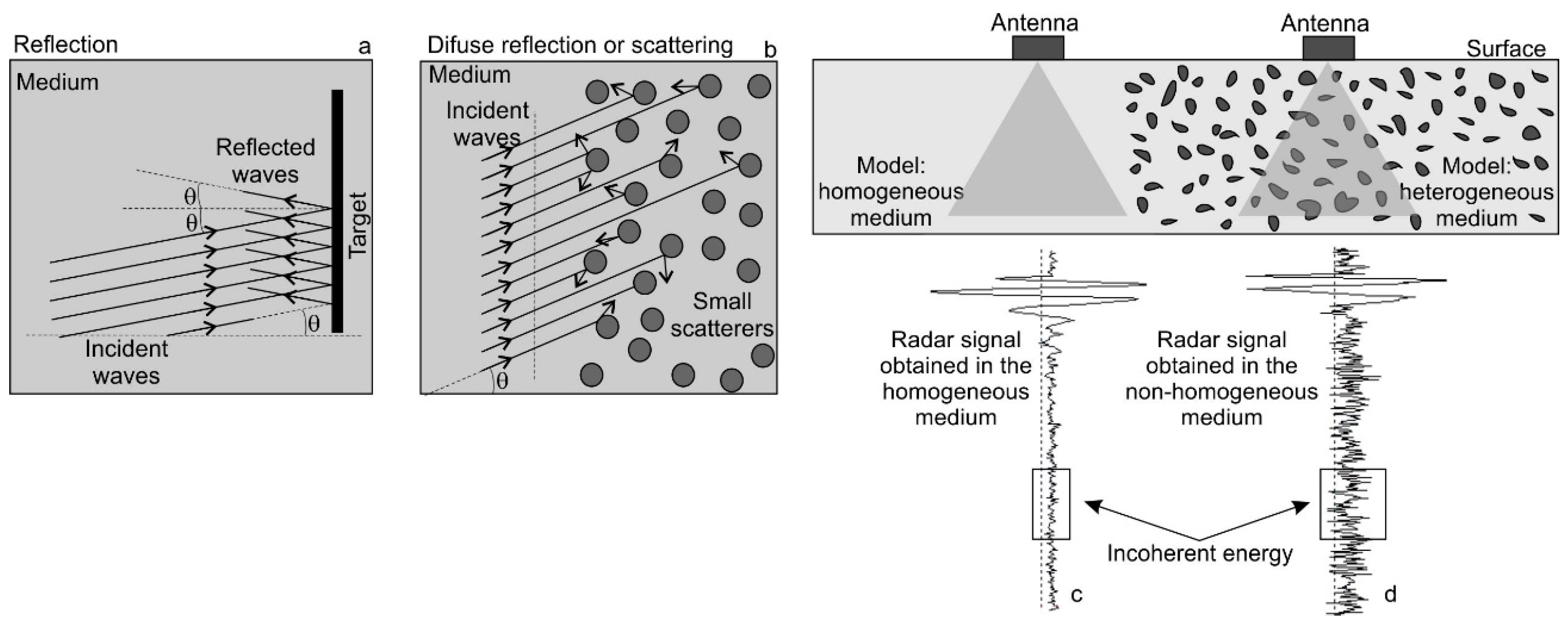
When the incident wave is perpendicular to a flat surface, the reflected wave returns with the same angle of incidence, being described the trajectory by the Law of Snell. However, in the case of a medium with a large number of scatterers which size is smaller than the wavelength, the scattering is described as the reflection of the wave in deviated trajectories in a random and not expected direction (Figure 1). This effect is similar in the case of incident waves on large rough surfaces.
Backscattering is defined as the amount of energy that is scattered back to the source and can be recorded by an antenna placed at the surface of the medium. The backscattered energy strongly depends on the size and the shape of the targets and big size targets can be considered as planar reflectors.
3. Heterogeneous Media and Targets with Rough Surfaces
The scattered energy depends on the heterogeneity of the medium or on the roughness of the targets or reflectors embedded in the medium. The Rayleigh criterion allows distinguishing between rough and smooth targets. In the case of a planar wave incident on an irregular and rough target with an angle α, the difference of phase, , between two rays scattered from different points of the surface is:
Being h the difference of height between the two points of the rough surface of the target embedded in the medium where the scattering is produced, β the incidence angle and λ the wavelength of the electromagnetic wave.
The Rayleigh criterion considers a non-smooth target surface when the phase difference is:
In that case, the parameter h could be defined depending mainly on the frequency or wavelength of the incident wave:
The approach of nearly vertical incident waves allows to approximate the heterogeneity size h as:
The phenomenon of dispersion and scattering in rough target surfaces has been analysed by several authors ([27,28,29]). The most usual approaches are the Kirchoff Approximation and the Small Perturbation Model (SPM). The Kirchoff approximation assume that the roughness dimensions of the target surface are large compared to the incident wavelength (Bragg scattering region), while the SPM model undertakes that the roughness is small compared to the wavelength. Therefore, the SPM model is more appropriate for long wavelengths as in the present GPR study, where the radiation is mainly in the I-band (IEEE bands), being the frequency lower than 200 MHz (which represent wavelengths up to 1.5 m). The approach assumes that the parameter h is small compared to the wavelength. In this case, the variation on the height of the targets’ surface is small compared to the wavelength and depending on the incident angle, the SPM decomposes the backscattered waves into their Fourier spectrum components.
4. Mean Amplitude of Incoherent Energy
Experimental GPR measurements in areas where high scattering was expected showed an important increase of the clutter in all A-scans [15]. Therefore, in order to relate the clutter with the heterogeneities of the medium, a procedure was developed to enhance the clutter associated to backscattered energy in dispersive targets, applied to the field surveys. The diffuse reflection in these heterogeneities increases the background noise (clutter) in GPR A-scans (see Figure 1). The analysis of the amplitude of this background energy could provide alternative information about changes in the ground, related to the homogeneity of the materials.
In the case of scattering in small particles or in rough surface, it is possible to assume that, for a specific time t, the total electromagnetic field arriving to the receiver can be expressed as the sum of the reflected () and the scattered () fields:
The wave front reflected on high-contrast permittivity surfaces, as well as multiple reflections returns to the receiver as coherent energy. This energy is predominant at short times of the radargram time window due to its great amplitude. At higher times, the amplitude of coherent reflections diminishes due to losses as consequence of previous reflections, geometrical spreading and absorption. Therefore, at a certain time, those amplitudes present similar magnitude than the amplitude of incoherent energy recorded as background noise in the A-scan, as consequence of clutter produced by random backscattering. In addition, that incoherent energy is most likely close to the diffuse regime because the energy arrives from all heterogeneities after being scattered a random number of times following unsystematic paths. This energy becomes predominant in the radar record when the amplitude of the coherent energy decreases in the case of high depth reflectors. A threshold time tS —in which the predominant field role exchanges—is defined comparing incoherent and coherent energies. This threshold time depends on each particular case studied and must be experimentally determined by comparing amplitudes. Using this parameter, the energy in the B-scans can be split in two zones:
The changes on the random backscattering must be examined for times t > tS, since analysing data in a properly selected time window (usually [tS, 2tS]) prevents the consideration of important reflections in targets. Notwithstanding, coherent energy is yet present but can be diminished by applying a subtract average, that reduce it in front of the incoherent energy. The quantitative analysis of the relative density of heterogeneities that perturbs the trace could be a methodology to define different zones in the ground.
The analysis of the B-scans region for times higher than ts is based on the definition of a single amplitude value that corresponds to the average of the energy recorded in the region. This value was corrected with gain to diminish the effects of geometrical spreading and absorption.
The Mean Amplitude of Incoherent Energy (MAIE) is defined for trace i as:
where is the amplitude of the incoherent energy in the selected time window after corrections and filters.
5. Field Data Processing
The processing is divided in three main parts: pre-processing, trace processing and final representation of MAEI versus position (Figure 2). Firstly, the wave velocity in the medium is determined to estimate the dielectric permittivity and consequently, to define the absorption losses. Two methodologies are applied in this part: comparing the GPR images to boreholes and analysing the hyperbolas along each B-scan. In this second case, it is possible to obtain the field of velocities, selecting an average value.
Secondly, the radargram is pre-processed. This pre-processing consists of a gain correction, a band pass filter with cut-off frequencies 10 MHz and 55 MHz. Data are also processed with demean and detrend before applying a subtract average.
Thirdly, this processing is focused to determine an average value of the amplitude within a 300 ns and 600 ns time window.
The last step of the processing consists of the normalization of the amplitude depending on the geological characteristics, being the normalization depending on a previous geological zonation. Finally, all MAEI values are represented over the position of the traces.
6. Application to Heterogeneous Media
The proposed method was applied in the city of Barcelona (Spain) which is built on a quaternary sedimentary basin. The objective was to determine changes in the ground, associated to variations in the heterogeneity of the medium. The ground of the basin was crossed by many subterranean and seasonal streams and paleochannels. These geological structures are composed by heterogeneous clusters of alluvial sediments in the zones corresponding to the streambeds. As consequence of these heterogeneities, it is expected an increase of the randomly backscattered energy, raising the amplitude of the background noise in the A-scans. Radar data was acquired with a 25 MHz centre frequency antenna. Therefore, the scattering was expected for clusters with sizes of 60 cm or less (Equation (6)). The results obtained from the study of the clutter amplitude caused by backscattering were compared to boreholes, to other geophysical measurements and also to cartographic information from ancient and modern maps.
As mentioned above, the first step was determining an average wave velocity in the medium, comparing the GPR results with known borehole data and with hyperbolas caused by shallow targets. A velocity of about 12 cm/ns was obtained as a mean result along the radar lines [30].
The second step was the application of a gain correction for spherical losses, using the two-way travel time and the velocities. An additional gain was also used to diminish the effects of the energy loss caused by absorption. In this case, the attenuation coefficient was determined by using the approximation of a dielectric and low-losses medium ():
where is the conductivity (an approximate value of 0.3 mS/m was used in the study), is the angular frequency, is the dielectric permittivity (between 6 and 7) and is the magnetic permeability (that was approximated to the unit).
The third step was the application of a band pass filter with cut-off frequencies 10 MHz and 55 MHz. After that processing, the subtracting average was applied to both radargrams (the processed one with the band pass filter and the non-processed one). The results are shown in Figure 3.
The fourth step was selecting the most appropriate time window. Figure 4 shows one of the radar images obtained in one radar line that crosses one of the seasonal subterranean streams of the zone, compared with a map. This image shows that the maximum depth of the anomalies related to anthropogenic constructions is less than 300 ns. This two-way travel time was used to determine the upper limit for the time window, being the lower limit 600 ns. This second value was chosen in order to avoid possible baseline deviations that could increase the level of the background noise amplitude.
The fifth step consists of calculating the absolute value of the amplitude (Figure 5).
The absolute amplitude was normalized based in the maximum amplitude value, comparing all the radar profiles acquired at the same geological unit in the selected time-window. The relative amplitude corresponding to any A-scan is normalized at each geological unit by rescaling the average amplitude determined at the time-window of this A-scan, . This averge amplitude is determined using the minimum and maximum amplitude values in the same time-window, comparing all A-scans acquired on the same geological zone:
In this case, the relative amplitude reaches a value 0 when the average amplitude of the time window is equal to the minimum amplitude (assumed as the intrinsic material mean amplitude) and a value 1 when it is equal to the maximum value observed for the clutter’ amplitude.
The last step was determining the average normalized amplitude of the clutter in the time-window. Finally, this amplitude was represented versus the distance along the radar lines acquired in the street (Figure 6).
The final result of the study includes the analysis of the average amplitudes obtained in all the B-scans that were acquired over the same geological unit.
6.1. Numerical Models
Numerical modelling is a proper method for evaluating the field results, comparing the real images to the numerical ones. The objective of the numerical simulation is to recreate the results of the GPR survey, mainly the backscattering phenomenon under the emission of electromagnetic waves (e.g., [29,31]). The effect takes place mainly under two different conditions: (1) when targets embedded in homogeneous medium present rough surfaces, being the roughness smaller than the wavelength; and (2) when the homogeneous medium is next to a more heterogeneous medium, being the size of the heterogeneities smaller than the wavelength. The presence of scatterers embedded in the homogeneous medium was modelled using the commercial software GPRSim©. This software was developed by the Geophysical Archaeometry Laboratory (Woodland Hills, CA, USA) and it is based on the ray tracing method. The basis and method is widely described in [32]. The software built a synthetic B-scan based on the response of the antenna and the wave type. The modelled medium is digitized into a grid of cells. Each cell contains the parameters defining the electromagnetic properties and also the coefficients of a polynomial function that describes the structural interfaces through the grid cell, allowing an infinite number of possible slope determinations. The synthetic radargram is determined from the rays that are sent into the grid of cells with an initial direction and amplitude, defined from the radiation pattern of the antenna.
Simulation was focused in the evaluation of the second condition, in order to recreate the real field ground. In the GPR field study, the ground was characterized by abrupt changes in the size of particles embedded in the medium as consequence of the existence of subterranean streams and paleochannels. Two models were used in two different computer analyses. The first simulation (called S1) is based in a well-defined band of scatterers and the second simulation (called S2) is based on scatterers in a band embedded in a material with randomly distributed particles (see Figure 7).
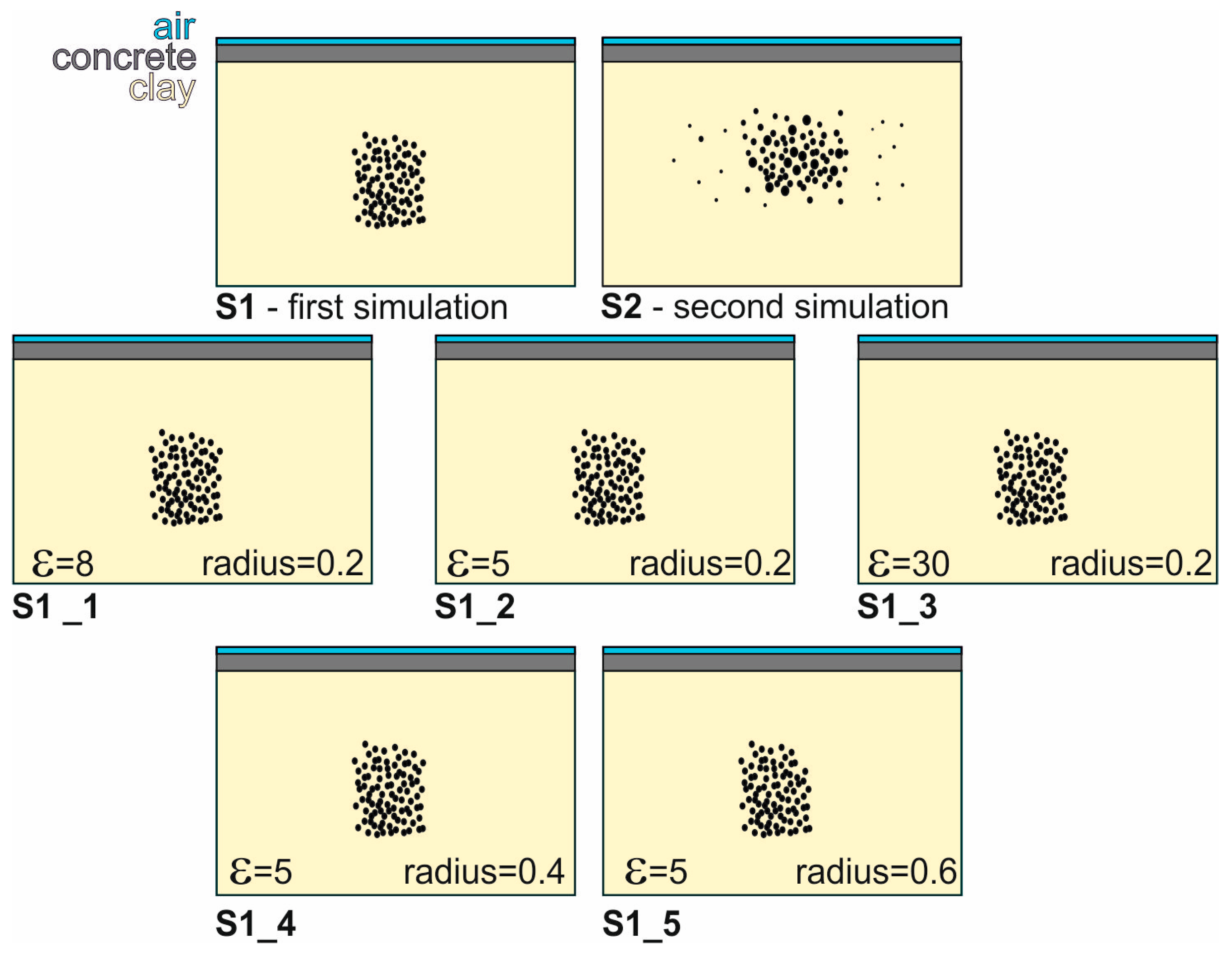
The first simulation (S1) of this second condition was studied for three cases, depending on the particles materials. The three cases are based on a simple flat layered structure [Air-Concrete-Clays dry] and the scatterers are randomly distributed in clusters, reproducing the field study conditions in Barcelona. The first stratum is a thin 0.15 cm air layer. The second stratum is a 1.5 m concrete layer (assuming man-made structures), placed over a wider stratum simulating dry clay. Scatterers represent small size targets (0.2 m, 0.4 m and 0.6 m radii) embedded in the third material. Three cases were considered, changing the targets dielectric constants (5, 8 and 30). The values were selected according to the expected values of most common geological materials in the zone. The geometrical distribution of those particles, 10 m to 20 m length restricted bands, intend to replicate the targets (underground seasonal streams and paleochannels) existing in the real medium. In the first case (Figure 7 and Figure 8b), the particles represent dry clay with a slight change in the dielectric permittivity between the matrix and scatterers. In the second case (Figure 7 and Figure 8c) the particles simulate dry sand and in the third case (Figure 7 and Figure 8d) the scatterers represent wet sand. Three different scatterers size are simulated for the same dry sand material. The dielectric constant, electrical conductivity and scatterers radii for the different materials considered in the models are shown in Table 1. Figure 7 presents the scheme of the models for the different computer simulations.
Synthetic traces were obtained every 0.5 m for a set of 5 cases using the same geometrical model in order to carry out a parametric study. In this model, spherical scatterers were randomly distributed into a restricted zone (x = [20, 30] m; y = [10, 30] m). Their position remains fixed for all the cases, which is shown in Figure 7 and Figure 8.
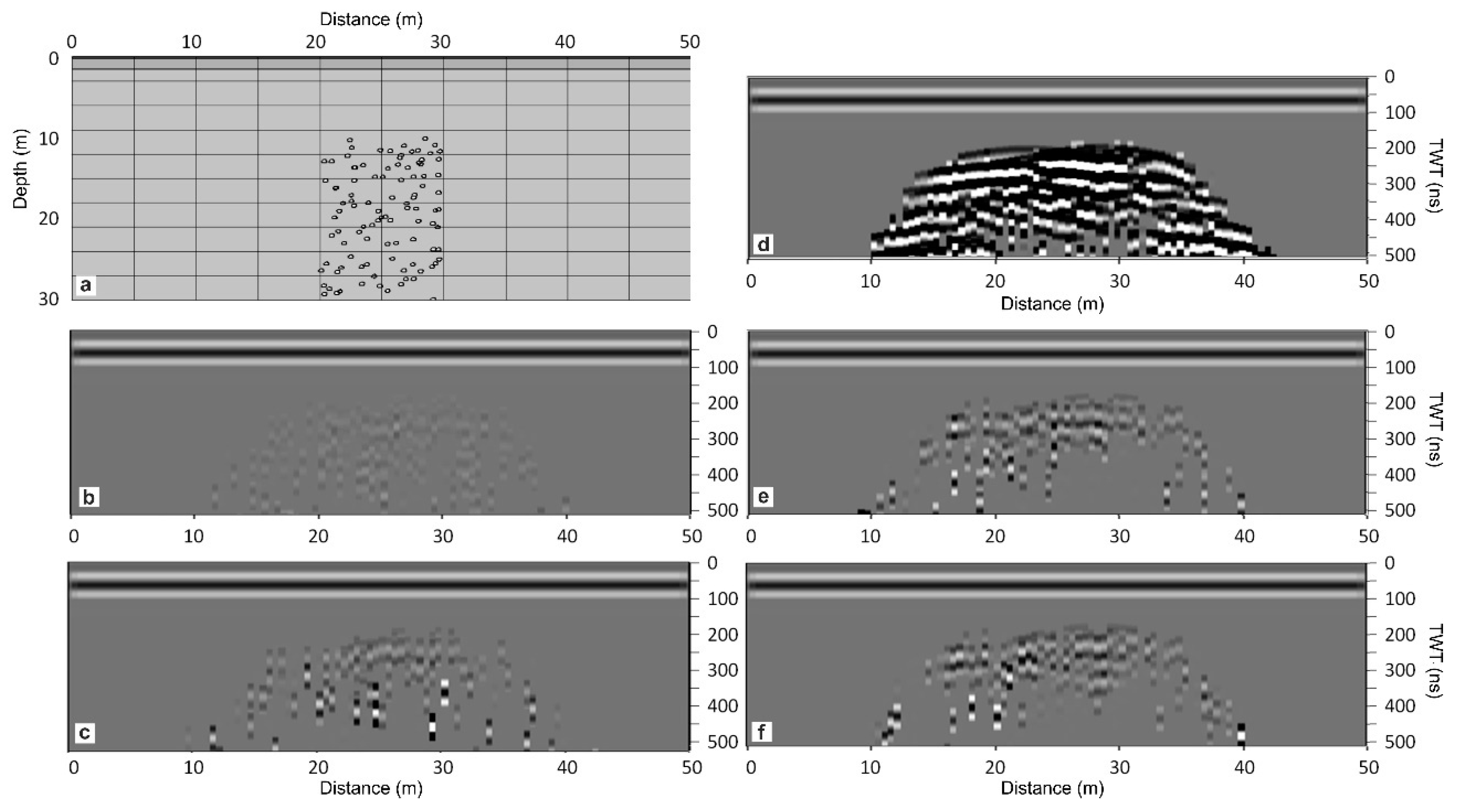
The results of the first simulation show significant backscattering appearing as consequence of scatterers, even in the case of small difference between the dielectric permittivity of the medium and scatterers. In the case of a greater contrast in the dielectric permittivity (Figure 8d), the synthetic image seems to be produced by a single and irregular target instead of a random distribution of small and individual scatterers. In the case of a larger particle size with the same dielectric permittivity, a slight increase of the backscattering amplitude is noticeable, depending on the radius (Figure 8c,e,f).
Additionally, differences in the radii of the scatterers introduce slight changes on the dispersed amplitudes. Notwithstanding, part of the energy observed in the model with the greater radius (S1_5) at higher times (≈300 ns) should be neglected in the backscattering analysis since it seems to be coherent with boundary reflections.
Other aspect to be considered when comparing to the field B-scans is the width of the area in the synthetic B-scans affected by the backscattering phenomenon. The antenna path produces images in which the wide of the scatterers band does not correspond to the real particle distribution. Shallower particles are detected before the antenna is placed over the band of scatterers.
The second simulation (S2) includes two kinds of scatterers. On one hand, 100 scatterers simulate clay and 0.1 m radius are randomly distributed through the entire clay layer, being the difference in dielectric permittivity very small between particles and matrix. These scatterers represent intrinsic heterogeneities of the layer. On the other hand, for a restricted zone (x = [20, 30] m; y = [5, 25] m) 300 spherical sand scatterers were randomly spread, being their radii randomly selected between 0 and 0.3 m. In this case, the traces were acquired every 0.1 m.
Results (see Figure 9) show that the mean amplitude of the incoherent energy increases when the antenna crosses the band of heterogeneities. In addition, synthetic images present a transition zone of about 5 m at each side of that zone, showing anomalies with an amplitude of about 15% of the maximum value. At higher times, the contribution of the early transmitted phases up to 3 collisions (TRT, TRRT, TTRT, TRRRT, TTRTT...) is smaller compared to the multi-scattered energy.
6.2. Comparison between GPR Survey and Passive Seismic
GPR was applied to locate those areas with high number of scatterers and field results were compared to computational models. In addition, the survey was also compared to passive seismic measurements and borehole data is specific zones of the profiles. Horizontal to Vertical Spectral Ratio (HVSR) is a passive seismic methodology, applied in many cases to determine the thickness of ground materials (e.g., [33,34]) and to map site effects (e.g., [23,35,36,37]). A wide description of the methodology and the application can be found in [30,38]. In these maps, each zone is characterized by the mean value of the predominant period. In the surveyed area, there are zones due to underground streams and paleochannels that represent sudden lateral changes in the shallow geology. These geological structures modify the predominant period. Figure 10 exhibits the location of the GPR survey line in Mallorca Street, the passive seismic measurements and the location of three boreholes near the surveyed zone. Boreholes show 15 m of Quaternary materials, approximately, being deeper the anthropogenic fill near the underground stream.
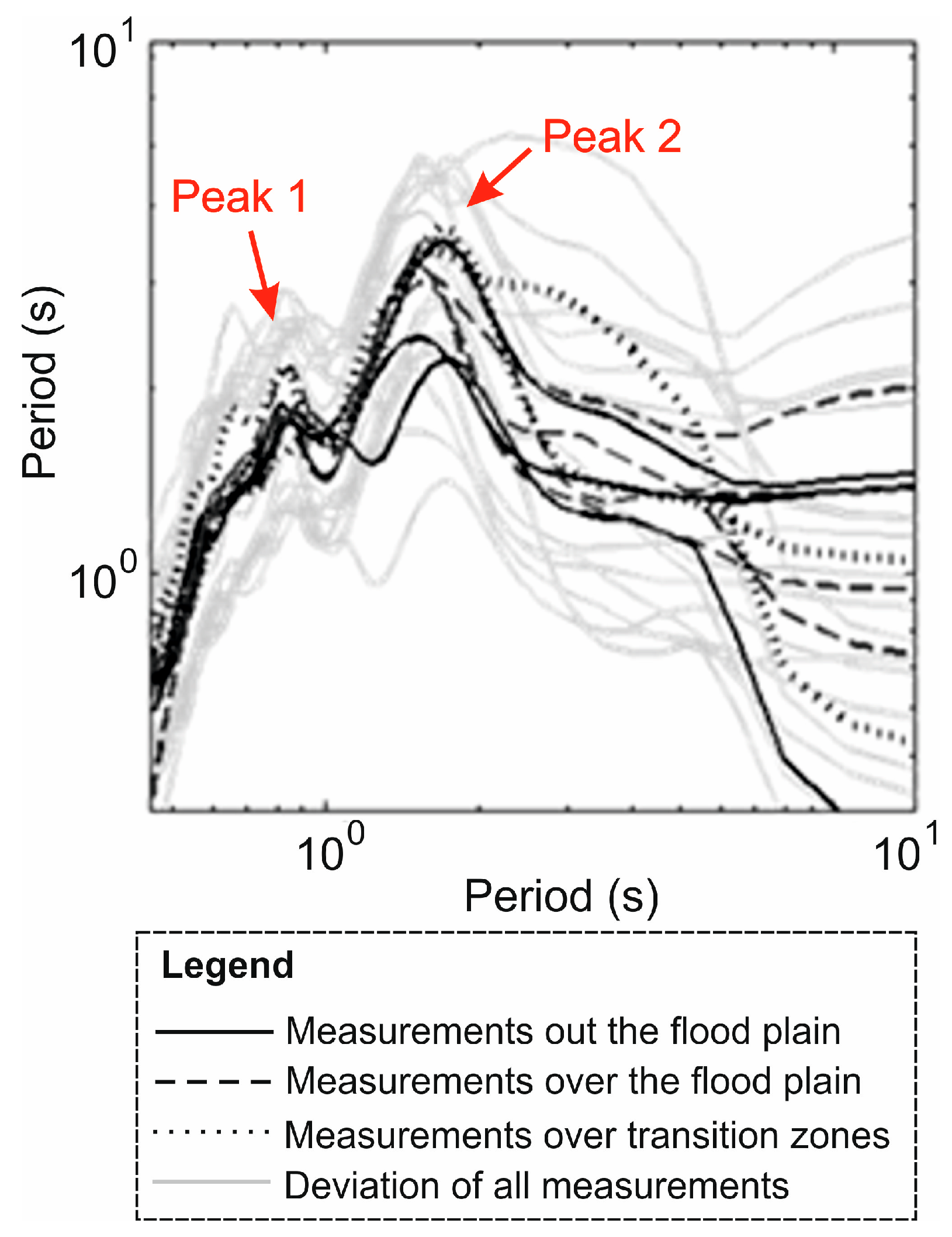
Passive seismic results were tested in different zones previous the measurements in the area of interest. HVSR results obtained near the subterranean streams present in the most cases a double peak in the H/V spectra, increasing also the mean amplitude and the period ([39]). In the particular study of Mallorca Street, a typical double peak denotes the presence of the geological structure associated to the stream (Figure 11). The location of these changes corresponds to the zones of the high backscattering amplitude in GPR B-scans being the results of the survey according to the GPR previous analysis and to the wide anthropogenic fill.
6.3. Discussion and Conclusions
This work described a processing technique based in enhancing the amplitudes associated to random backscattering energy, avoiding the coherent reflections in targets. This method quantified relatively this energy among the different traces, allowing defining zones where this phenomenon is produced.
The application of the procedure to a real scenario shows the correlation between the increase of the clutter in the A-scans at higher times and the existence of subterranean streams. This increase of clutter is most likely consequence of the random scattering of the energy in clusters of small targets corresponding to alluvial deposits.
The analysis of the wave velocity in the case study provides a value near 12 cm/ns. The wavelength in the medium, based in this velocity is about 480 cm. Therefore, assuming the conditions for scattering presented in the paper, the threshold size of the heterogeneities that cause this effect is close 60 cm. Hence, most likely, changes in the clutter amplitude are not caused by changes in the size of sedimentary particles but in the existence of clusters of granular materials, characteristics of fluvial deposits. Most likely, the area historically affected by the subterranean stream is composed by this kind of deposits of materials, being the main cause of the increase of clutter at higher propagation times.
Two simulations have been done in order to compare and validate the results of this procedure in the subsoil evaluations. First, the influence of the grain size and the composition of the scatterers were analysed by means of a parametric study. Comparing the synthetic results obtained in the case of different parameters (grain size and composition), it was observed that amplitudes are strongly dependent on the contrast of impedance between scatterers and surrounding materials. Additionally, the amplitude is higher as the radius of particles grows. However, more analysis could be needed in order to obtain quantitative results.
In the second simulation, there was a higher synthetic trace density and the model included two kinds of scatterers. One of them was distributed randomly in the ground layer, representing the intrinsic layer heterogeneity. The other kind of scatterers represented the clusters, modelling alluvial deposits. The results in this second simulation indicates that the clutter at higher times corresponding to random backscattering increased when the emission and reception of the energy was over the cluster of particles. Moreover, the synthetic radar data showed a transition zone where the backscattering amplitude is increasing from the average value obtained distant from the cluster to the average amplitude obtained over the cluster. Those transition zones were also observed at the case study. Therefore, that result could indicate that the experimental evaluations overestimate the real flood plain that is interpreted in the radargrams as a more extended zone than the real anomalous geological structure. Otherwise, the results of the simulation could indicate that the higher amplitudes obtained through this processing are produced mainly as consequence of multi-scattering.
Concluding, the analysis of the amplitude of clutter caused by random scattering is revealed as a useful tool to distinguish particular sedimentary structures that are not properly identified by anomalies caused by coherent reflections of the energy. The evaluation of the amplitudes at a concrete time window allows the detection of those particular changes in the subsoil.
The results of the proposed methodology indicate the potential of GPR to define sudden changes in the shallow geology in a quick survey. Comparing GPR results to passive seismic measurements, the zones defined by means of the GPR clutter could be most likely defined by the same seismic soil response. Therefore, the GPR method can be applied as a previous evaluation, before the passive seismic measurements. Those preliminary results could help in reducing the number of passive seismic measurements, which are time consuming. In addition, the previous definition of possible zones will increase the accuracy of the final results.
The analysis developed in the current work, could be further extended to other fields such as Civil Engineering, to be used to detect granular accumulation particles in concrete, or non-homogeneous mixture in highways pavements, with the final objective to map pathologies.
Acknowledgments
This research has been partially funded by the Ministry of Economy and Competitiveness (MINECO) of the Spanish Government and by the European Regional Development Fund (FEDER) of the European Union (UE) through projects referenced as: CGL2011-23621 and CGL2015-65913-P (MINECO/FEDER, UE). The study is also a contribution to the EU funded COST Action TU1208, “Civil Engineering Applications of Ground Penetrating Radar”.
Author Contributions
All the authors contribute equally in the radar data acquisition, interpretation and writing the paper. Victor Salinas acquired and interpreted the seismic data. Victor Salinas and Vega Perez-Gracia prepared the computer simulation. Sonia SantoS-Assunçao and Vega Perez-Gracia prepared the processing flow. The three authors contribute in the paper preparation and revision.
Conflicts of Interest
The authors declare no conflict of interest.
References
- Annan, A.P. GPR—History, trends, and future developments. Subsurf. Sens. Technol. Appl. 2002, 3, 253–270. [Google Scholar] [CrossRef]
- Daniels, D.J. Ground Penetrating Radar, 2nd ed.; The Institution of Electrical Engineers: London, UK, 2004; 726p. [Google Scholar]
- Jol, H.M. (Ed.) Ground Penetrating Radar Theory and Applications; Elsevier: Amsterdam, The Netherlands, 2008. [Google Scholar]
- Davis, J.L.; Annan, A.P. Ground-penetrating radar for high-resolution mapping of soil and rock stratigraphy. Geophys. Prospect. 1989, 37, 531–551. [Google Scholar] [CrossRef]
- Busby, J.P.; Merritt, J.W. Quaternary deformation mapping with Ground Penetrating Radar. J. Appl. Geophys. 1999, 41, 75–91. [Google Scholar] [CrossRef]
- Grasmueck, M.; Weger, R.; Horstmeyer, H. Three-dimensional ground-penetrating radar imaging of sedimentary structures, fractures, and archaeological features at submeter resolution. Geology 2004, 32, 933–936. [Google Scholar] [CrossRef]
- Benson, A.K. Applications of ground penetrating radar in assessing some geological hazards: Examples of groundwater contamination, faults, cavities. J. Appl. Geophys. 1995, 33, 177–193. [Google Scholar] [CrossRef]
- Arcone, S.A.; Lawson, D.E.; Delaney, A.J.; Strasser, J.C.; Strasser, J.D. Ground-penetratinng radar reflection profiling of groundwater and bedrock in an area of discontinuous permafrost. Geophysics 1998, 63, 1573–1584. [Google Scholar] [CrossRef]
- Ulugergerli, E.U.; Akca, İ. Detection of cavities in gypsum. J. Balk. Geophys. Soc. 2006, 9, 8–19. [Google Scholar]
- Mochales, T.; Casas, A.M.; Pueyo, E.L.; Pueyo, O.; Román, M.T.; Pocoví, A.; Soriano, M.A.; Ansón, D. Detection of underground cavities by combining gravity, magnetic and ground penetrating radar surveys: A case study from the Zaragoza area, NE Spain. Environ. Geol. 2008, 53, 1067–1077. [Google Scholar] [CrossRef]
- Grasmueck, M. 3-D ground-penetrating radar applied to fracture imaging in gneiss. Geophysics 1996, 61, 1050–1064. [Google Scholar] [CrossRef]
- Porsani, J.L.; Sauck, W.A.; Júnior, A.O. GPR for mapping fractures and as a guide for the extraction of ornamental granite from a quarry: A case study from southern Brazil. J. Appl. Geophys. 2006, 58, 177–187. [Google Scholar] [CrossRef]
- Sun, J.; Young, R.A. Recognizing surface scattering in ground-penetrating radar data. Geophysics 1995, 60, 1378–1385. [Google Scholar] [CrossRef]
- Grimm, R.E.; Heggy, E.; Clifford, S.; Dinwiddie, C.; McGinnis, R.; Farrell, D. Absorption and scattering in ground-penetrating radar: Analysis of the Bishop Tuff. J. Geophys. Res. Planets 2006, 111. [Google Scholar] [CrossRef]
- Santos Assunçao, S. Ground Penetrating Radar Applications in Seismic Zonation: Assessment and Evaluation. Ph.D. Thesis, Universitat Politècncia de Catalunya, Barcelona, Spain, 2014; 284p. [Google Scholar]
- Vuksanovic, B.; Bostanudin, N.J.F. Clutter removal techniques for GPR images in structure inspection tasks. In Proceedings of the Fourth International Conference on Digital Image Processing (ICDIP 2012), Kuala Lumpur, Malaysia, 7–8 April 2012; International Society for Optics and Photonics: Bellingham, WA, USA, 2012; p. 833413. [Google Scholar]
- Chen, C.S.; Jeng, Y. A data-driven multidimensional signal-noise decomposition approach for GPR data processing. Comput. Geosci. 2015, 85, 164–174. [Google Scholar] [CrossRef]
- Wang, X.; Liu, S. Noise suppressing and direct wave arrivals removal in GPR data based on Shearlet transform. Signal Process. 2017, 132, 227–242. [Google Scholar] [CrossRef]
- Santos-Assuncao, S.; Perez-Gracia, V.; Salinas, V.; Caselles, O.; Gonzalez-Drigo, R.; Pujades, L.G.; Lantada, N. GPR Backscattering Intensity Analysis Applied to Detect Paleochannels and Infilled Streams for Seismic Nanozonation in Urban Environments. IEEE J. Sel. Top. Appl. Earth Obs. Remote Sens. 2015, 9, 167–177. [Google Scholar] [CrossRef]
- Al-Qadi, I.L.; Xie, W.; Roberts, R. Scattering analysis of ground-penetrating radar data to quantify railroad ballast contamination. NDT E Int. 2008, 41, 441–447. [Google Scholar] [CrossRef]
- Benter, A.; Moore, W.; Antolovich, M. GPR signal attenuation through fragmented rock. Min. Technol. 2016, 125, 114–120. [Google Scholar] [CrossRef]
- Perez-Gracia, V.; Caselles, O.; Salinas, V.; Pujades, L.G.; Clapés, J. GPR applications in dense cities: Detection of paleochannels and infilled torrents in Barcelona GPR applications in dense cities. In Proceedings of the IEEE 13th International Conference on Ground Penetrating Radar (GPR), Lecce, Italy, 21–25 June 2010; pp. 1–5. [Google Scholar]
- Salinas, V.; Caselles, J.O.; Pérez-Gracia, V.; Santos-Assunçao, S.; Clapes, J.; Pujades, L.G.; González-Drigo, R.; Canas, J.A.; Martinez-Sanchez, J. Nanozonation in dense cities: Testing a combined methodology in Barcelona City (Spain). J. Earthq. Eng. 2014, 18, 90–112. [Google Scholar] [CrossRef] [Green Version]
- Pettinelli, E.; Burghignoli, P.; Pisani, A.R.; Ticconi, F.; Galli, A.; Vannaroni, G.; Bella, F. Electromagnetic propagation of GPR signals in Martian subsurface scenarios including material losses and scattering. IEEE Trans. Geosci. Remote Sens. 2007, 45, 1271–1281. [Google Scholar] [CrossRef]
- Reichman, J. Determination of absorption and scattering coefficients for nonhomogeneous media. 1: Theory. Appl. Opt. 1973, 12, 1811–1815. [Google Scholar] [CrossRef] [PubMed]
- Harbi, H.; McMechan, G.A. Conductivity and scattering Q in GPR data: Example from the Ellenburger dolomite, central Texas. Geophysics 2012, 77, H63–H78. [Google Scholar] [CrossRef]
- Beckmann, P.; Spizzichino, A. The Scattering of Electromagnetic Waves from Rough Surfaces; Artech House, Inc.: Norwood, MA, USA, 1987; 511p. [Google Scholar]
- Soldovieri, F.; Hugenschmidt, J.; Persico, R.; Leone, G. A linear inverse scattering algorithm for realistic GPR applications. Near Surf. Geophys. 2007, 5, 29–41. [Google Scholar] [CrossRef]
- Takahashi, K.; Igel, J.; Preetz, H. Modeling of GPR clutter caused by soil heterogeneity. Int. J. Antennas Propag. 2012, 2012, 643430. [Google Scholar] [CrossRef]
- Santos-Assuncao, S.; Perez-Gracia, V.; Gonzalez-Drigo, R. GPR backscattering applied to urban shallow geology: GPR application in seismic microzonation. In Proceedings of the IEEE 8th International Workshop on Advanced Ground Penetrating Radar (IWAGPR), Florence, Italy, 7–10 July 2015; pp. 1–4. [Google Scholar]
- Takahashi, K.; Igel, J.; Preetz, H.; Sato, M. Sensitivity analysis of soil heterogeneity for ground—Penetrating radar measurements by means of a simple modeling. Radio Sci. 2015, 50, 79–86. [Google Scholar] [CrossRef]
- Goodman, D. Ground-penetrating radar simulation in engineering and archaeology. Geophysics 1994, 59, 224–232. [Google Scholar] [CrossRef]
- Chandler, V.W.; Lively, R.S. Utility of the horizontal-to-vertical spectral ratio passive seismic method for estimating thickness of Quaternary sediments in Minnesota and adjacent parts of Wisconsin. Interpretation 2016, 4, SH71–SH90. [Google Scholar] [CrossRef]
- Picotti, S.; Francese, R.; Giorgi, M.; Pettenati, F.; Carcione, J.M. Estimation of glacier thicknesses and basal properties using the horizontal-to-vertical component spectral ratio (HVSR) technique from passive seismic data. J. Glaciol. 2017, 63, 229–248. [Google Scholar] [CrossRef]
- Caselles, J.O.; Pérez-Gracia, V.; Franklin, R.; Pujades, L.G.; Navarro, M.; Clapes, J.; Canas, J.A.; García, F. Applying the H/V method to dense cities. A case study of Valencia City. J. Earthq. Eng. 2010, 14, 192–210. [Google Scholar] [CrossRef]
- Panzera, F.; D’Amico, S.; Lombardo, G.; Longo, E. Evaluation of building fundamental periods and effects of local geology on ground motion parameters in the Siracusa area, Italy. J. Seismol. 2016, 20, 1001–1019. [Google Scholar] [CrossRef]
- Qadri, S.T.; Islam, M.A.; Shalaby, M.R.; Khattak, K.R.; Sajjad, S.H. Characterizing site response in the Attock Basin, Pakistan, using microtremor measurement analysis. Arab. J. Geosci. 2017, 10, 267. [Google Scholar] [CrossRef]
- Alfaro, A.; Pujades, L.G.; Goula, X.; Susagna, T.; Navarro, M.; Sanchez, J.; Canas, J.A. Preliminary Map of Soil’s Predominant Periods in Barcelona Using Microtremors. Pure Appl. Geophys. 2001, 158, 2499–2511. [Google Scholar] [CrossRef]
- Salinas, V. Detección Fina de Cambios Laterales en la Geología Superficial y en los Suelos y Caracterización de su Influencia en la Respuesta Sísmica Local. Aplicación a Barcelona (Exhaustive Detection of Lateral Changes in Surface Geology and in Soils and Characterization of Their Influence on the Local Seismic Response. Application to Barcelona). Ph.D. Thesis, Universitat Politècncia de Catalunya, Barcelona, Spain, 2015; 350p. (In Spanish). [Google Scholar]
Figure 1.
The clutter caused by small and irregular targets embedded in the medium increases the background noise in the A-scans. (a) Reflection in a flat target inside the medium; (b) Diffuse reflection is small scatterers embedded in the medium; (c) GPR A-scan obtained in homogeneous media; (d) GPR A-scan from a heterogeneous medium.

Figure 2.
Processing flow diagram.

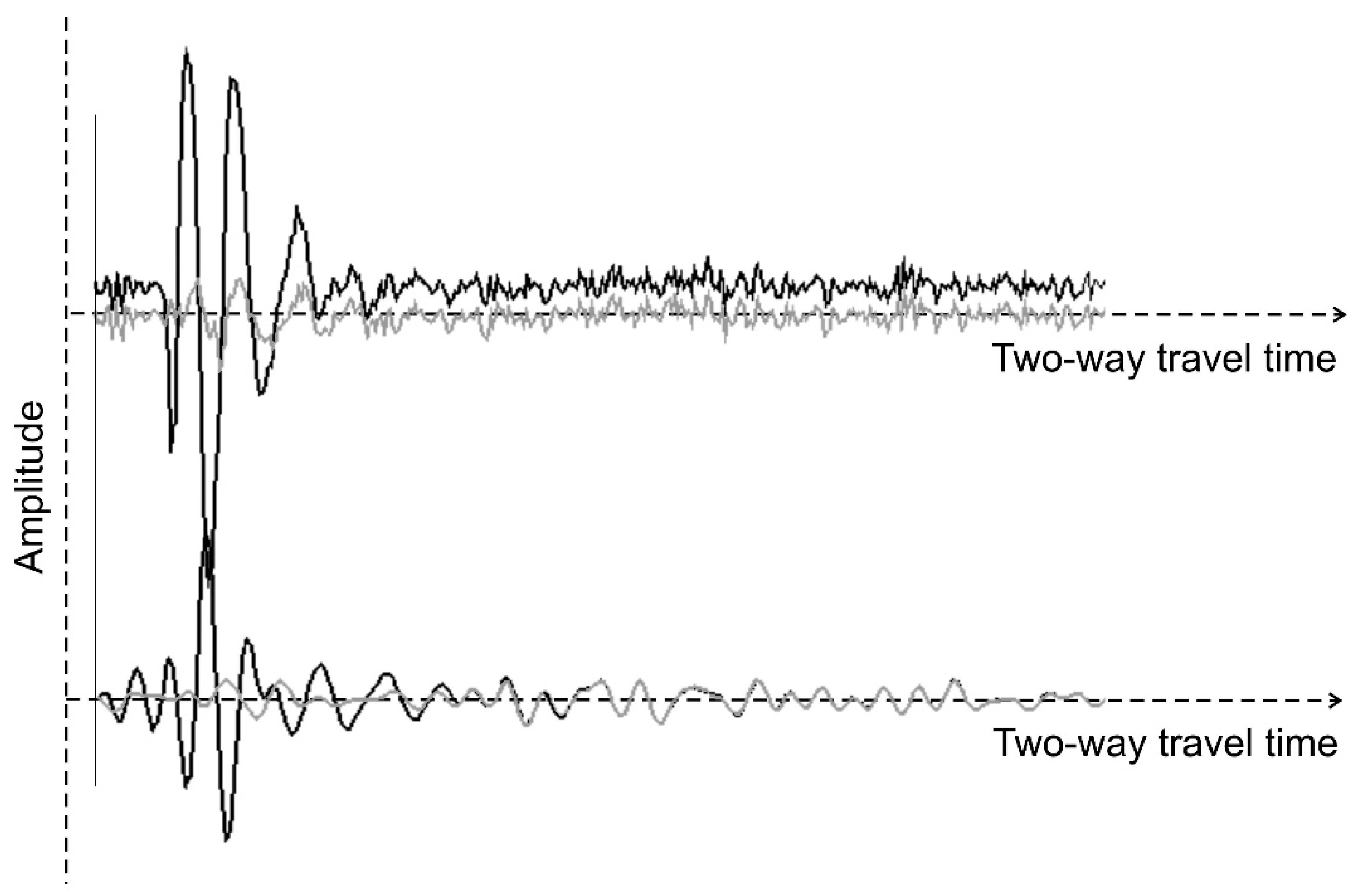
Figure 3.
The black A-scan is the original trace. The grey A-scan is the trace obtained after the subtracting average processing. Above, before the application of a band-pass filter. Below, after applying a band pass filter with cut-off frequencies 10 MHz and 55 MHz.
Figure 3.
The black A-scan is the original trace. The grey A-scan is the trace obtained after the subtracting average processing. Above, before the application of a band-pass filter. Below, after applying a band pass filter with cut-off frequencies 10 MHz and 55 MHz.

Figure 4.
Radar data along 270 m, showing the maximum two-way travel time (TWT) recorded for reflections on anthropogenic targets. The radar line crosses one subterranean stream in the area where the background noise at the B-scan is increased (between 120 m and 160 m).
Figure 4.
Radar data along 270 m, showing the maximum two-way travel time (TWT) recorded for reflections on anthropogenic targets. The radar line crosses one subterranean stream in the area where the background noise at the B-scan is increased (between 120 m and 160 m).
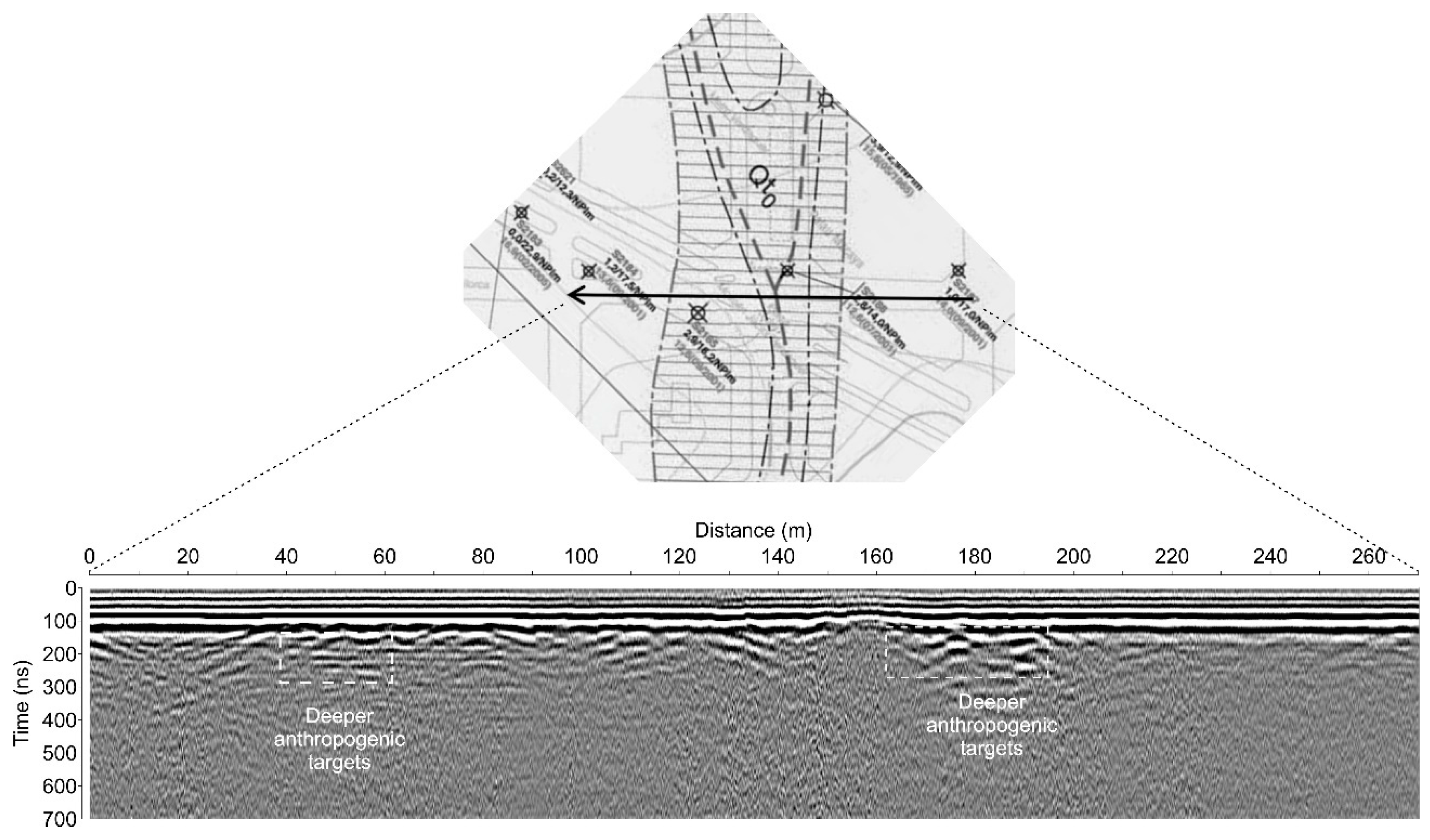
Figure 5.
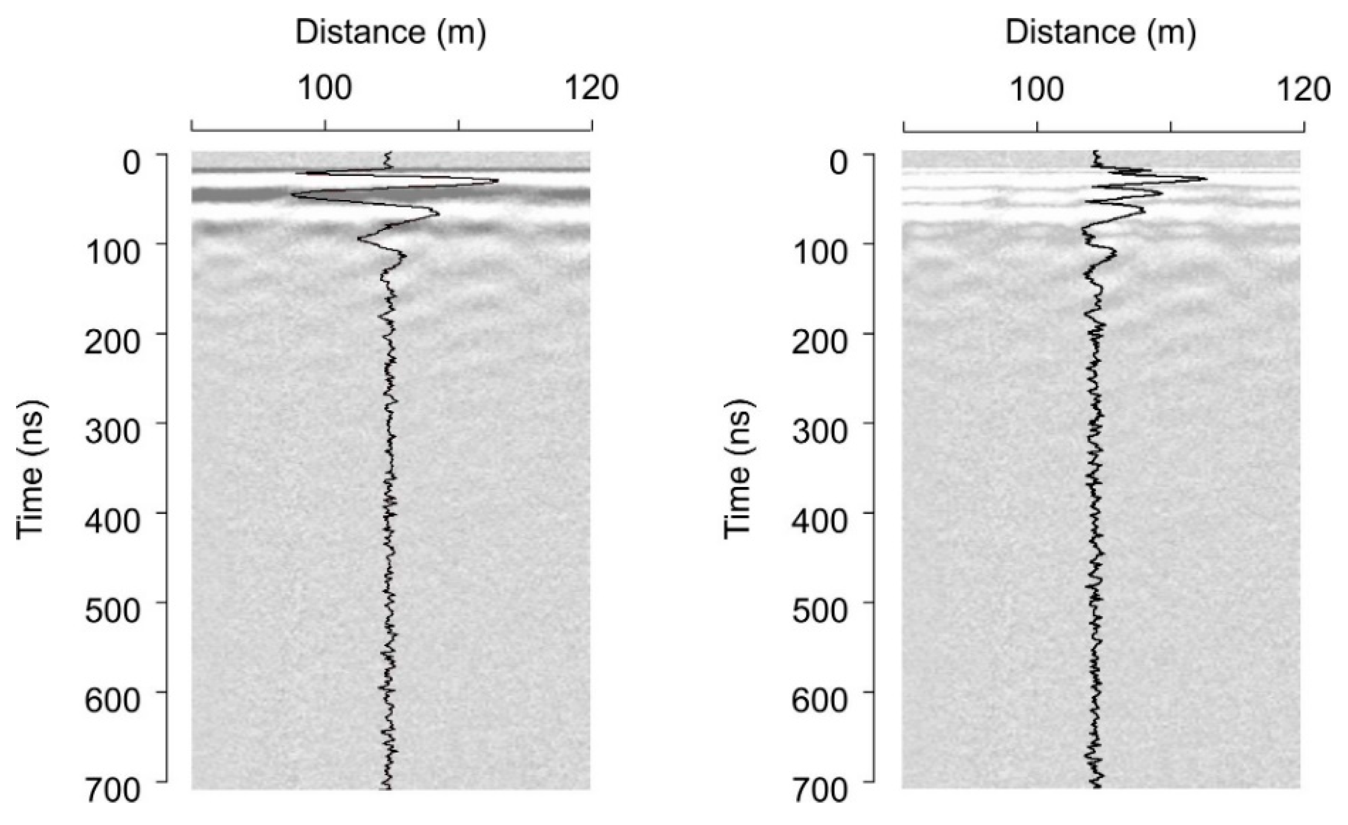
The first radargram presents A-scan and B-scan. The second radargram shows the absolute values of the A-scan and B-scan.
Figure 5.
The first radargram presents A-scan and B-scan. The second radargram shows the absolute values of the A-scan and B-scan.

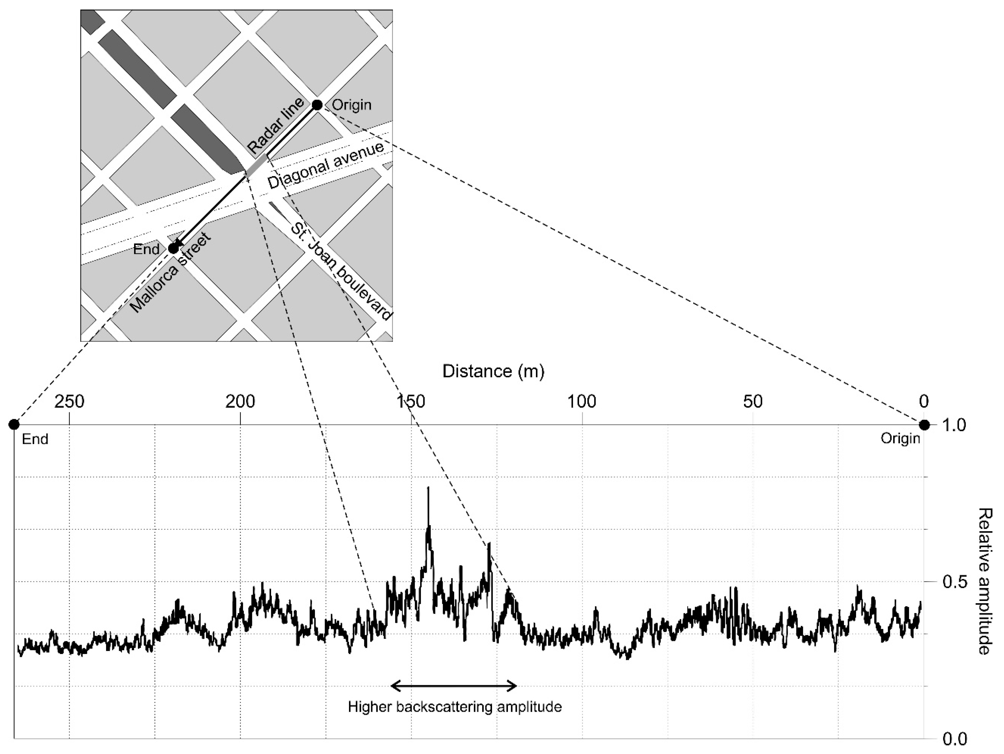
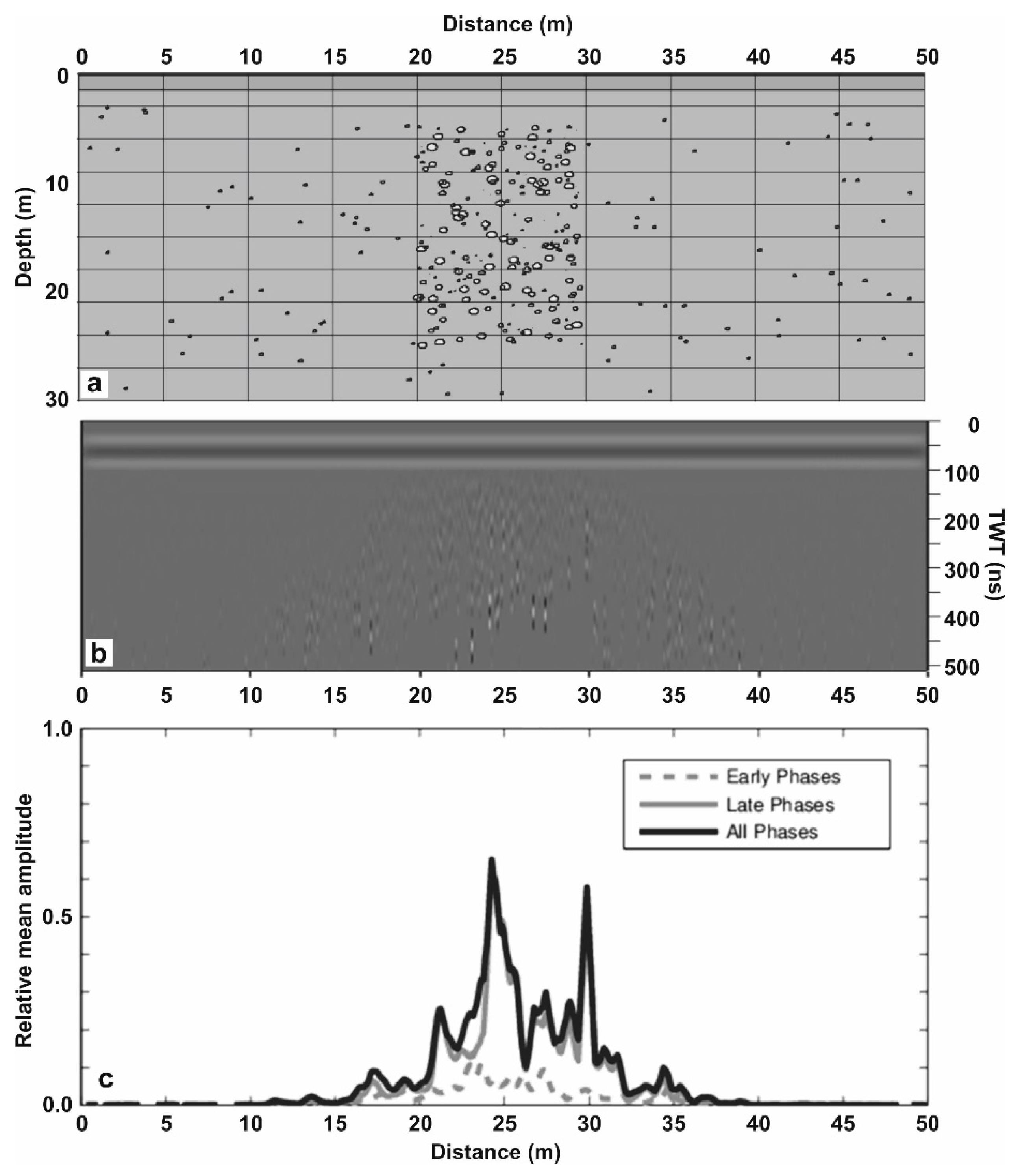
Figure 6.
Average relative amplitude in the time-window versus the distance along the radar line and location of the profile at the city map.
Figure 6.
Average relative amplitude in the time-window versus the distance along the radar line and location of the profile at the city map.

Figure 7.
The two simulations (S1 and S2) based on different particles distribution. S1_1, S1_2, S1_3, S1_4 and S1_5 represent the five sub-cases considered in the first simulation (S1).
Figure 7.
The two simulations (S1 and S2) based on different particles distribution. S1_1, S1_2, S1_3, S1_4 and S1_5 represent the five sub-cases considered in the first simulation (S1).

Figure 8.
Three layered model with the position of the 100 scatterers (a) and synthetic traces for: case S1_1 (b); case S1_2 (c); case S1_3 (d); case S1_4 (e) and, case S1_5 (f).
Figure 8.
Three layered model with the position of the 100 scatterers (a) and synthetic traces for: case S1_1 (b); case S1_2 (c); case S1_3 (d); case S1_4 (e) and, case S1_5 (f).

Figure 9.
(a) Model used in the second simulation; (b) synthetic traces and (c) mean amplitude of Incoherent Energy for the profile.
Figure 9.
(a) Model used in the second simulation; (b) synthetic traces and (c) mean amplitude of Incoherent Energy for the profile.

Figure 10.
Location of the seasonal underground stream, the GPR line, the passive seismic measurements and the boreholes.
Figure 10.
Location of the seasonal underground stream, the GPR line, the passive seismic measurements and the boreholes.
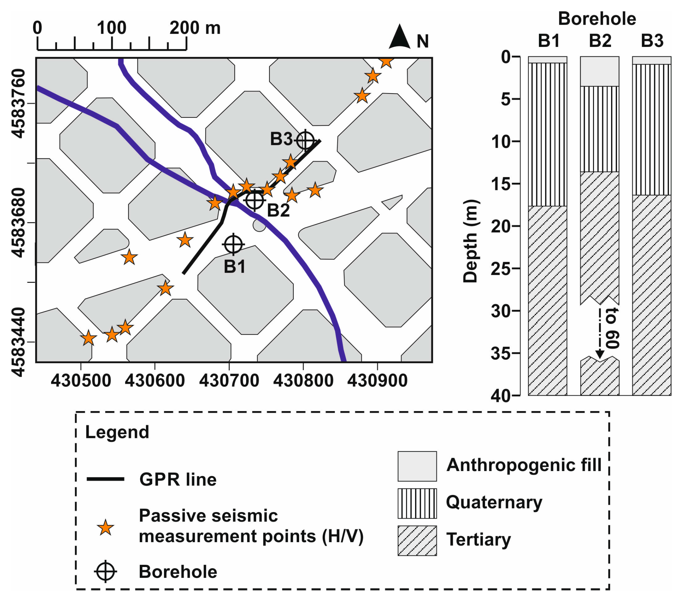
Figure 11.
Passive seismic results (horizontal to vertical spectra ratio) in the zone affected by the subterranean stream in Mallorca Street. The arrows indicate the double-peak.
Figure 11.
Passive seismic results (horizontal to vertical spectra ratio) in the zone affected by the subterranean stream in Mallorca Street. The arrows indicate the double-peak.


Table 1.
Characteristics of the scatterers in the five analysed cases.
| Model | Radius (m) | εr | S/m | Simulated Material |
|---|---|---|---|---|
| S1_1 | 0.2 | 8 | 0.0003 | Clays-Scatterer |
| S1_2 | 0.2 | 5 | 0.0001 | Dry Sand |
| S1_3 | 0.2 | 30 | 0.001 | Wet Sand |
| S1_4 | 0.4 | 5 | 0.0001 | Dry Sand |
| S1_5 | 0.6 | 5 | 0.0001 | Dry Sand |
© 2018 by the authors. Licensee MDPI, Basel, Switzerland. This article is an open access article distributed under the terms and conditions of the Creative Commons Attribution (CC BY) license (http://creativecommons.org/licenses/by/4.0/).
Share and Cite
MDPI and ACS Style
Salinas Naval, V.; Santos-Assunçao, S.; Pérez-Gracia, V. GPR Clutter Amplitude Processing to Detect Shallow Geological Targets. Remote Sens. 2018, 10, 88. https://doi.org/10.3390/rs10010088
AMA Style
Salinas Naval V, Santos-Assunçao S, Pérez-Gracia V. GPR Clutter Amplitude Processing to Detect Shallow Geological Targets. Remote Sensing. 2018; 10(1):88. https://doi.org/10.3390/rs10010088
Chicago/Turabian StyleSalinas Naval, Victor, Sonia Santos-Assunçao, and Vega Pérez-Gracia. 2018. "GPR Clutter Amplitude Processing to Detect Shallow Geological Targets" Remote Sensing 10, no. 1: 88. https://doi.org/10.3390/rs10010088
Note that from the first issue of 2016, this journal uses article numbers instead of page numbers. See further details here.