Identifying Generalizable Image Segmentation Parameters for Urban Land Cover Mapping through Meta-Analysis and Regression Tree Modeling


1
Natural Resources and Ecosystem Services Area, Institute for Global Environmental Strategies, 2108-11 Kamiyamaguchi, Hayama, Kanagawa 240-0115, Japan
2
Department of Geomatics Engineering, University of Isfahan, Isfahan 8158177361, Iran
*
Author to whom correspondence should be addressed.
†
These authors contributed equally to this study.
Remote Sens. 2018, 10(1), 73; https://doi.org/10.3390/rs10010073
Submission received: 10 November 2017
/
Revised: 20 December 2017
/
Accepted: 3 January 2018
/
Published: 6 January 2018
(This article belongs to the Special Issue Geographic Object-Based Image Analysis (GEOBIA))
Abstract
:The advent of very high resolution (VHR) satellite imagery and the development of Geographic Object-Based Image Analysis (GEOBIA) have led to many new opportunities for fine-scale land cover mapping, especially in urban areas. Image segmentation is an important step in the GEOBIA framework, so great time/effort is often spent to ensure that computer-generated image segments closely match real-world objects of interest. In the remote sensing community, segmentation is frequently performed using the multiresolution segmentation (MRS) algorithm, which is tuned through three user-defined parameters (the scale, shape/color, and compactness/smoothness parameters). The scale parameter (SP) is the most important parameter and governs the average size of generated image segments. Existing automatic methods to determine suitable SPs for segmentation are scene-specific and often computationally intensive, so an approach to estimating appropriate SPs that is generalizable (i.e., not scene-specific) could speed up the GEOBIA workflow considerably. In this study, we attempted to identify generalizable SPs for five common urban land cover types (buildings, vegetation, roads, bare soil, and water) through meta-analysis and nonlinear regression tree (RT) modeling. First, we performed a literature search of recent studies that employed GEOBIA for urban land cover mapping and extracted the MRS parameters used, the image properties (i.e., spatial and radiometric resolutions), and the land cover classes mapped. Using this data extracted from the literature, we constructed RT models for each land cover class to predict suitable SP values based on the: image spatial resolution, image radiometric resolution, shape/color parameter, and compactness/smoothness parameter. Based on a visual and quantitative analysis of results, we found that for all land cover classes except water, relatively accurate SPs could be identified using our RT modeling results. The main advantage of our approach over existing SP selection approaches is that our RT model results are not scene-specific, so they can be used to quickly identify suitable SPs in other VHR images.
1. Introduction
1.1. High-Resolution Remote Sensing and GEOBIA
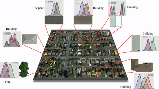
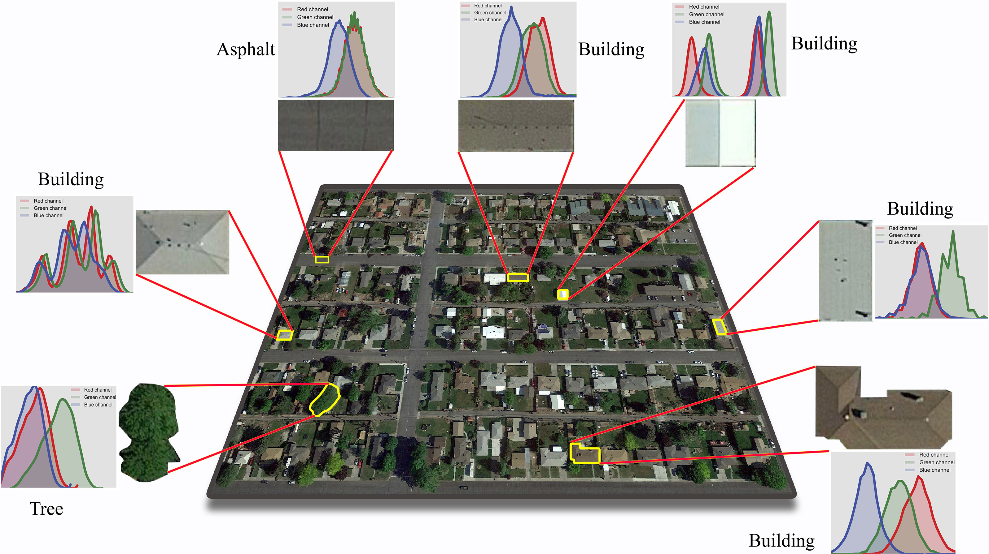
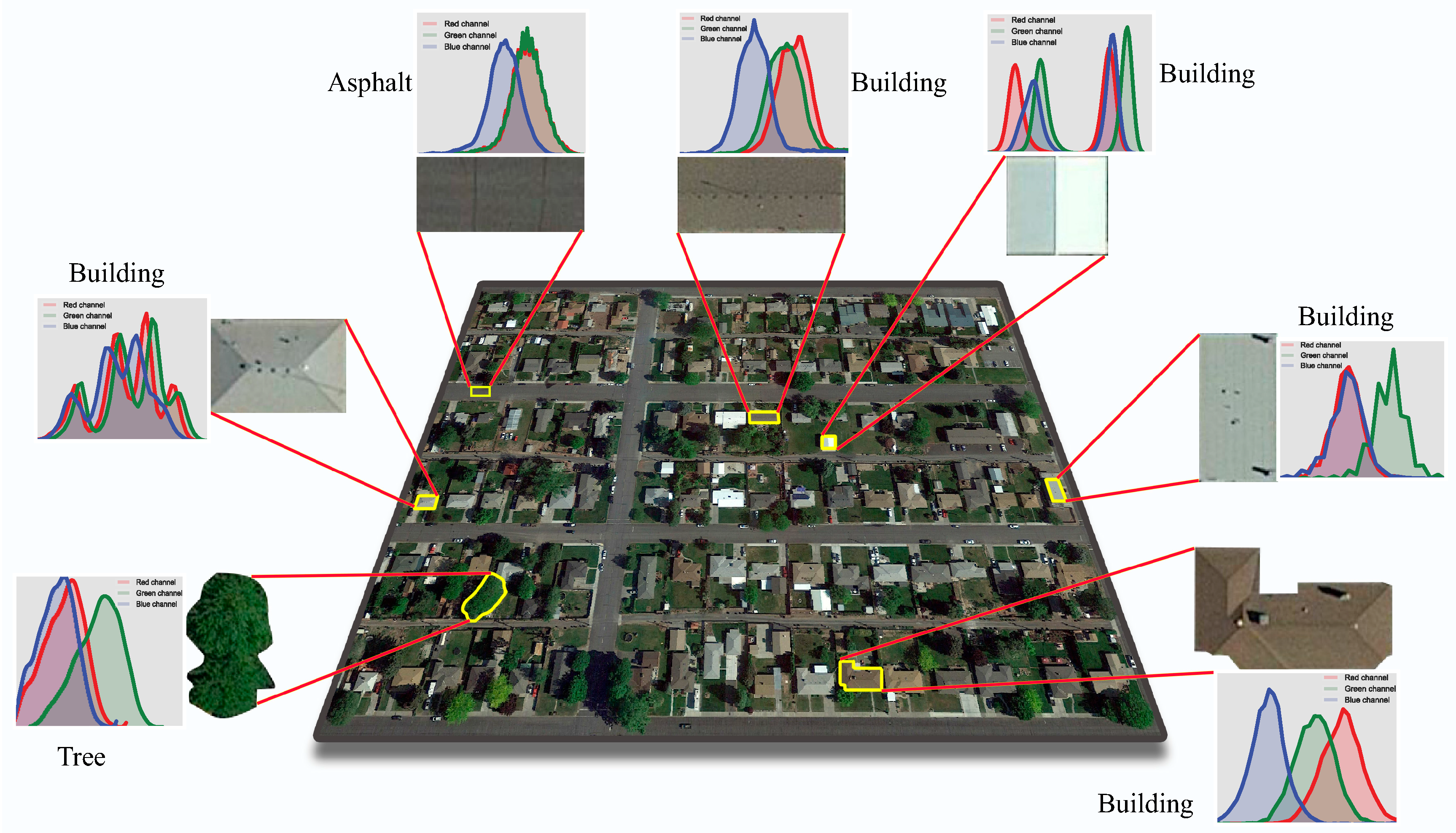
Fine scale urban land cover information is valuable for a wide range of applications, including the analysis of urban green space accessibility [1], urban hydrology [2], and urban heat island effect [3]. The advent of remote sensing and very high resolution (VHR) imagery has significantly facilitated the procedure for producing and updating urban land cover maps. However, the classification of urban land cover objects of interest (e.g., roads, buildings, trees, grass, bare soil) in VHR images based on their spectral properties is still very challenging due to the high within-class spectral heterogeneity and high between-class spectral similarity of many of these objects (Figure 1). For example, the materials and colors of building rooftops may vary widely, and some rooftops may have very similar spectral properties to roads. Due to these problems, traditional pixel-based approaches, which assume that each land cover class has a distinct spectral signature (and do not take into account other pertinent spatial/contextual information that helps correctly identify land cover features) [4,5], often fail to achieve a desirable level of classification accuracy. For these reasons, the geographic object-based image analysis (GEOBIA) approach, which is able to incorporate various types of spatial (e.g., objects’ texture and/or shape) and context (e.g., multi-scale spectral/spatial features) information for classification, is often used for high-resolution urban land cover mapping [6,7,8]. In addition, in several studies it was shown that applying the GEOBIA framework to medium spatial resolution imagery can lead to promising results [5,9,10].
The GEOBIA process typically involves: (i) segmenting a remote sensing image into spectrally homogeneous regions (i.e., segments or image objects), and (ii) utilizing the spectral, spatial, and/or context features of these segments for image classification (Figure 2). Many image segmentation algorithms exist [11,12,13], but perhaps one of the most commonly used for remote sensing applications is the multiresolution segmentation (MRS) algorithm [14,15], which was first implemented in the eCognition software package (Trimble Geospatial).
1.2. Multiresolution Segmentation (MRS) Algorithm
The MRS algorithm has three free parameters that must be set for segmentation: a “scale parameter” (SP) that controls the maximum heterogeneity of each segment, a “smoothness/compactness” parameter that determines the preferred shape of segments, and a “color/shape” parameter that controls the weights of spectral and shape information in the calculation of segments’ heterogeneity [15]. One of the most significant properties of MRS is its ability to generate the same results for different subsets selected from the same area [15]. This capability in reproducing segmentation results distinguishes MRS from some other common segmentation algorithms [13]. Through an optimization process, MRS divides a given image into relatively homogeneous regions, i.e., image segments or image objects. The relationship between the user-defined SP (S) and the inter-segment heterogeneity cost function (f) can be expressed as follows:
- If f < S2, then merge the two image segments
- If f ≥ S2, then do not merge the two image segments
The parameters of MRS are typically estimated through a trial-and-error process; that is, the analyst applies different parameter settings to the image under consideration until meaningful and desired objects are extracted. The trial-and-error process for determining the parameters can be both time-consuming and labor-intensive due to the lack of an explicit relationship between a segmentation result and the three parameters. In general, SP is considered as the most important driver of yielding a desired segmentation because it indirectly governs the average size of resulting image objects [16]. However, the meaning of the SP in MRS is to some degree ambiguous because it only provides an implicit and irreproducible association (i.e., the larger the SP is, the bigger the average size of segments is), which is not a practical tool for generating optimal segmentation results. To address these problems, over the past decade a number of supervised and unsupervised automatic approaches to parametrizing the MRS SP (as well as the parameters of other segmentation algorithms) have been proposed.
Since each object that is present in a given image could have different characteristics (e.g., its size, shape, color, etc.) from other objects, a single SP is not often useful to extract all types of land covers in the image. If a universal SP is applied, it is likely that many objects will be either oversegmented or undersegmented. As already discussed, in either case the accuracy of classification results can be deteriorated, because some important information is not available during the classification phase. In fact, objects’ inherent characteristics have an important role in finding suitable SPs. The selection of an SP to segment the image should be based on the geometric/spectral properties of the object(s) of interest. As a result, to extract different land cover classes, it is more reasonable to use multiple SPs, each of which is appropriate for a separate land cover class. Such a multi-scale/level approach can positively affect the quality of extraction of different land cover classes, and thus can improve the accuracy of final classification results, as reported in several studies [17,18,19,20].
1.3. Segmentation Parameter Selection
Past research has shown that land cover classification accuracy can be affected by the settings of the segmentation parameters [19,21,22,23,24], so care must be taken to ensure that the parameters set do not result in excessive undersegmentation (i.e., segments much larger than the objects of interest) or oversegmentation (i.e., segments much smaller than the objects of interest). In practice, multiple segmentation parameters are usually tested and compared, and “suitable” segmentation parameters (i.e., those that do not cause excessive over- or undersegmentation) are determined either manually (by trial and error [25,26,27]) or automatically (e.g., using supervised or unsupervised parameter selection algorithms [17,20,22,28,29,30,31]). Although manual parameter selection through visual assessment could lead to the most optimal segmentation results if done by a skilled image analyst, the process is typically time consuming and/or computationally intensive. Moreover, since this process could be tedious, the analyst may rely on his/her prior knowledge to choose the parameters, which could increase the subjectivity of the process [32].
It is often claimed that the segmentation parameter selection process is needed because good segmentation parameters vary by image source (e.g., QuickBird, WorldView-2/-3, Pléiades) and by study area location [17,33,34]. However, to our knowledge, there has been no comprehensive study of how much these good segmentation parameters vary. If a relatively narrow range of good segmentation parameters could be identified for similar types of images (e.g., images from the same satellite sensor or images with similar spatial resolutions), this could potentially reduce the time needed for parameter selection (a narrower range of parameters would need to be compared) or even eliminate the need for it (if the range of parameters has very little variation).
Recently, Ma et al. [35] conducted a comprehensive meta-analysis on common considerations taken into account in GEOBIA studies. They examined 173 scientific papers and extracted several parameters from each study including image spatial resolutions, selected SPs, classifiers, land cover types, sampling methods, etc. One of the other factors they analyzed from this meta-analysis was the relationship between the selected SP in each study and the spatial resolution of the imagery used in the study. The main limitation of this analysis in the previous work was that it did not assess the relationship between SP and image spatial and radiometric resolutions for different types of land cover. However, this is important because not all land cover classes can be accurately segmented using a single SP [19,36].
1.4. Objective of This Study
Similarly to the study by Ma et al. [35], our current study also aimed to take advantage of the results of past research to improve the efficiency of future GEOBIA research. Specifically, we aimed to reduce the time/effort needed for setting appropriate MRS parameters for different urban land cover types, with a focus on VHR (<5 m) imagery, which was previously shown to be effective for urban mapping [37,38]. As reported by Cowen et al. [39], to recognize an urban object in a given remotely sensed image, the spatial resolution should be at least one-half of the smallest object to be extracted. For example, to identify an urban building with a size of 10 m × 10 m, the minimum spatial resolution must be 5 m. However, Myint et al. [37] argued that for urban applications, it is recommended to choose a spatial resolution even finer than one-half the size of the smallest object. As the authors elaborated in the abovementioned study, if the pixel size is not finer than one-half the size of the object of interest, some pixels (those containing the boundaries of the object) will not be completely composed of the objects (i.e., mixed pixels), so that the accuracy of extracting them will be degraded. In this regard, we performed a meta-analysis of recent GEOBIA literature to assess the variation in segmentation parameters used for urban land cover mapping in various types of images and locations, with the goal of determining if a relatively narrow range of good segmentation parameters could be identified for different types of images and land covers. The main research question we wanted to answer with this meta-analysis was whether appropriate MRS parameters (especially SP) were indeed site-specific. For this analysis, we: (1) performed a literature survey of recent studies from 2010 to 2017 (21 June) involving the use of GEOBIA for urban land cover mapping; (2) extracted the segmentation parameters used, image source/spatial and radiometric resolutions, etc., in each study; and (3) built a regression tree (RT) model for each individual land cover type using the extracted information to investigate how well the segmentation parameters (specifically SP) selected in the past studies could be predicted based on the image data used (e.g., spatial and radiometric resolutions).
2. Related Work
Studies on parametrizing SP can be categorized into two general groups: supervised approaches [21,30,31,40], and unsupervised approaches [17,20,22,29]. With supervised methods, the goal is to identify an optimal segmentation (or set of segmentations) by evaluating the overlap of ground-truth reference polygons and computer-generated image segments. This evaluation is performed using arithmetic or geometric dissimilarity metrics to calculate the discrepancy between reference polygons and the respective (overlapping) generated segments. When these metrics indicate the least dissimilarity between a given ground truth and the overlapping segment, it could be concluded that an optimal segmentation has been achieved. Liu et al. [40] proposed three discrepancy metrics (i.e., Potential Segmentation Error (PSE), Number-of-Segments Ratio (NSR), and Euclidean Distance 2 (ED2)) for the supervised optimization of MRS parameters. In that study, PSE was defined as a measure of undersegmentation (i.e., a PSE value equal to zero indicates no undersegmentation), NSR as a measure of oversegmentation (i.e., larger values of NSR indicate oversegmentation occurred), and ED2 was used to combine the other two metrics into a single value that takes into account both undersegmentation and oversegmentation (i.e., the smaller the value of ED2 is, the more the resulting segments match the corresponding reference polygons). In another study, Clinton et al. [41] compared several different supervised metrics and combinations approaches, and found that the D-metric, calculated as the root-mean-square of an oversegmentation measure (OverSegmentationij or OSeg) and an undersegmentation measure (UnderSegmentationij or USeg), was consistently a good indicator of segmentation quality. In a further work, Zhang et al. [42] used similar undersegmentation/oversegmentation measures, and compared different approaches for combining them (F-measure, Euclidean Distance, ED2), and found that F-measure was more appropriate for combining the undersegmentation and oversegmentation metrics together due to its higher sensitivity to excessive under-/oversegmentation.
In contrast to supervised methods, unsupervised SP optimization methods can be applied without the need for reference polygons. Many unsupervised methods aim to identify the segmentation parameters that maximize the average intra-segment heterogeneity and inter-segment homogeneity of segmentation results [29]. Compared to supervised methods, unsupervised techniques can potentially be faster (not requiring reference polygons) and less subjective. Aside from the methods based on maximizing intra-segment heterogeneity/inter-segment homogeneity, Drǎgut et al. [28] developed a method known as the Estimation of Scale Parameter (ESP) tool, which was inspired by the concept of Local Variance (LV) that earlier proved to be beneficial for recognizing the structure of a given image with respect to its spatial resolution and land cover [43], and for applying to the GEOBIA framework [44]. The basis on which the ESP tool is built is that as larger SPs are used for segmenting a given image, the average global standard deviation (as a representative of LV) of the spectral values of image segments increases accordingly. This increase in the average standard deviation stops when the boundaries of some image segments approximately correspond to a real-world feature. By monitoring the LV curve resulting from this approach, it can be observed that several break points appear on the curve, and each of these abrupt changes can be indicative of an optimal SP for the corresponding land cover. As a result, using the ESP tool it is possible to estimate multiple SPs for various image objects with different sizes and structures.
Parameterizing the MRS algorithm has also been carried out using the notion of spatial autocorrelation in some studies [45,46,47]. Spatial autocorrelation is important in the sense that it effectively reveals the statistical separability of spatial image objects from each other [45]. Martha et al. [47] made use of the objective function (composed of a spatial autocorrelation indicator (i.e., Moran’s I) and inter-segment variance analysis) proposed by Espindola et al. [45] to develop a plateau objective function (POF) capable of constraining the lower limit of the objective function for detecting multiple optimal SPs. The authors hypothesized that the peak values of the POF are close to the maximum values of the objective function. Thus, it can be concluded that a trade-off between oversegmentation and undersegmentation in the results can be found where the peaks exceeding the constrained lower limit of the objective function are observed; that is, such a trade-off indicates an optimal SP for the image under consideration. In addition, the local peaks on the curve of the objective function can be indicative of optimal SPs for land features with different sizes in the image. Johnson and Xie [29] proposed another multi-scale approach that estimates optimal segmentations in two steps, namely a global evaluation step, and a local evaluation step. Optimal segmentations are selected by normalizing and combining (through addition) weighted variance (for evaluation of intra-segment heterogeneity), and Moran’s I (for evaluation of inter-segment heterogeneity). Following that study, Johnson et al. [22] found that combining the Weighted Variance and Moran’s I metrics using the F-measure was more effective than combining them using addition, which echoed the findings by Zhang et al. [42] that the F-measure was more sensitive to excessive over- and undersegmentation. In a more recent study, Cánovas-García and Alonso-Sarría [48] adapted the method introduced by Espindola et al. [45] and developed a local SP optimizing technique by replacing the Moran’s I index with the Geary index (as an intra-segment heterogeneity measure) to also include objects’ variability when optimizing the SP. The main advantage of their method is its local optimization nature (uniform spatial units) that is beneficial in cases where the study area is large and covers diverse types of land use/cover. The main reason that local approaches could typically lead to more desirable results is that they can better capture the spectral contrast between objects than global approaches can, thus yielding more appropriate SPs [19].
In 2014, Yang et al. [49] developed a multiband unsupervised approach based on measuring the spectral homogeneity of image segments generated to estimate appropriate SP automatically. According to their study, as the size of an image object increases, its corresponding spectral homogeneity continues to decrease until it conforms to a real-world object. Therefore, measuring spectral homogeneity can be considered as a proxy for objectively estimating the SP. In order to measure spectral homogeneity, the authors adopted spectral angle [50]. The spectral angle indicates the amount of similarity between two pixels; that is, the more the two pixels are similar to each other, the smaller the value of the spectral angle is. Based on this fact, Yang et al. [49] first calculated the spectral angle between each pair of two pixels in each segment. Then, the calculated mean spectral angle values of all the pairs of two pixels for each segment were averaged over the entire image. Finally, the SP resulting in the smallest value of mean spectral angle (i.e., the largest spectral homogeneity) was considered as an optimal SP.
In a recent study, Jozdani et al. [20] developed a scene-independent unsupervised approach to optimizing the SP to extract urban buildings of different sizes. In that research, by assuming that the sizes of buildings in a given urban block are close to each other, a degree-2 polynomial regression model was established that associated appropriate SPs with the median size of buildings and the spatial resolution of the image. According to their experiments, it is possible to estimate appropriate multiple SPs to quickly extract differently sized buildings with reasonable accuracy and without relying on intensive computations.
In addition to the abovementioned approaches, other methods have been proposed that do not heavily rely on the SP to optimize segmentation. For instance, Martha et al. [51] first performed an initial segmentation with a small SP to generate oversegmented results. These oversegmented results were then fed into the chessboard segmentation algorithm to be fine-tuned and merged, resulting in more appropriate final segmentation results without directly optimizing the SP. In a similar study, Witharana and Lynch [31] combined the segmentation derived from the multi-threshold segmentation (MTS) algorithm with that derived from the MRS to improve segmentation results without applying an intensive trial-and-error process. In their method, MTS is first applied to the image to generate undersegmented, simplified image objects. Subsequently, MRS is performed on the simplified segments to obtain finer image objects whose boundaries more reasonably correspond to real-world features of interest. Finally, a straightforward trial-and-error process can be applied to the segmentation results of the MRS to further fine-tune image objects generated.
Rather than hybridizing the MRS algorithm with other segmentation algorithms to optimize segmentation and to improve classification accuracy, in a study by Stumpf and Kerle [52], the main objective was to identify which features were more significant at each scale level to improve final classification results in the GEOBIA framework (in this case, distinguishing landslides from other image objects). For this purpose, they first performed multiple segmentations with different SP values (i.e., 10, 15, 20, 25, 30, 35, 40, 45, 50, 55, 60, 70, 80, 90, and 100) and then calculated several features (i.e., spectral, textural, geometric, etc.) for the resulting image objects at different scale levels. Following this step, an RF-based variable-importance model was applied to the calculated features to recognize significant features at each segmentation level that could lead to more accurate classification results, namely smaller out-of-bag (OOB) error resulting from the RF model. To put it simply, instead of solely taking the SP into account to improve the extraction of objects of interest, final classification accuracy can be considered as a function of the SP and significant features calculated for image objects generated.
Although unsupervised methods to optimize the SP/segmentation do not require reference polygons, they can be still computationally intensive. For example, most existing unsupervised approaches require iteratively testing many different SP values to identify an optimal segmentation, which can be problematic especially when segmenting a large volume of remotely sensed images. Even though the framework proposed by Jozdani et al. [20] avoids this iterative procedure, it is still limited to the appropriate extraction of urban buildings and thus cannot be generalized to other land covers in its current form.
3. Methodology
In this paper, we investigated the potential of mathematical modeling to estimate appropriate SPs for different urban land covers based on a meta-analysis. The main goal was to identify if suitable SP values could be found for several different land cover types using the information derived from past GEOBIA studies (e.g., what segmentation parameters were used for: different land cover types, different types of images, etc.?). The meta-analysis scheme in this study closely followed the pattern used by Ma et al. [35]. Accordingly, this research was organized into three main steps: (1) searching for relevant papers, (2) collecting information needed from each study, and (3) applying regression modeling to estimate suitable SPs for different land cover types.
3.1. Literature Survey
In the first step, a comprehensive survey of recent studies involving GEOBIA for urban land cover mapping was conducted. To find potentially relevant research papers, we used Scopus (http://www.scopus.com) and Google Scholar (http://www.scholar.google.com), which are web databases of peer-reviewed (and non-peer-reviewed) literature. The criteria and search terms used in these engines were as follows: “object-based” AND “urban” AND “land cover”, and the search was limited to peer-reviewed journal papers. We focused our investigation on urban areas because of the extensive application of the GEOBIA framework for urban area mapping using VHR imagery, and because of the challenging task of segmenting/classifying urban land cover (e.g., due to high within-class spectral heterogeneity and high between-class spectral similarity, other segment-level features like size/shape are very useful). We also focused only on studies published from 2010 to 2017 (the last search was performed on 21 June 2017), as it was during the time that the GEOBIA framework really became mainstream in remote sensing (an exponential increase in GEOBIA studies occurred starting from 2010) [35].
3.2. Extracting Image/Segmentation Parameter Information from Past Studies
The second step of our methodology was to extract the relevant information from each paper. For this purpose, information related to three types of parameters was collected from each paper:
- Image-based information
- MRS parameter information
- Land cover information
Each of these information groups plays an important role in the quality of a segmentation result. The image-based information included the spatial and radiometric resolutions of the images used in each research paper. The MRS parameter information comprised the SP, shape/color, and compactness/smoothness parameters used in each study. The land cover information collected included the land cover types corresponding to the MRS parameter settings in each study. The common land cover classes that presented in the considered studies were tree, grass, bare soil, impervious (including roads, asphalt, parking lots, etc.), building, water, road, and pool. It should be however underlined that in several studies, some details were missing. For example, some studies did not report any information on the spatial or radiometric resolutions, or on the MRS parameters used. In such cases, we assumed the default values for missing data (more details on this issue are given in Section 4).
3.3. Regression Analysis to Estimate Appropriate SP Values
The last step was to formulize the relationship between all the three information groups (i.e., image-based, the shape and compactness parameters, and land cover) and the SPs selected in the studies. In order to associate the SPs with the rest of the information extracted, we made use of regression modeling. In this respect, since the goal of this study was to narrow down the range of suitable SPs for different urban land cover types, regression modeling was performed for each type of land cover separately. The dependent variable was chosen to be SP used for segmenting the land cover class of interest, and the independent variables were chosen to be the shape parameter, compactness parameter, spatial resolution, and radiometric resolution. There are several regression models that can be used for prediction purposes. Generally, since the real-world relationships of different variables are rarely linear, nonlinear regression models can often yield more accurate predictions. In many remote sensing studies, complex nonlinear regression models (e.g., Artificial Neural Networks (ANN), Support Vector Regression (SVR), Random Forests (RF), etc.) have been able to achieve satisfactory results, but because they act as a black box (i.e., the procedures through which they are fitted to the data are hidden) their results are difficult to interpret. Moreover, they do not provide any explicit, reproducible equations that can be easily applied by other researchers (i.e., generalized). Because of these two problems, we did not use these types of complex models, even though they could possibly result in higher modeling accuracy. We instead utilized a regression tree (RT) approach to predict the SP values, as RTs can also be used for nonlinear regression modeling and provide interpretable/explicit relationships (in the form of rulesets) between the independent and dependent variables [44]. In general, an RT is a binary splitting process that recursively stratifies the feature space into sub-divisions. Stratification is based on the minimization of deviation from the mean of the response variable. The structure of this rule-based regression model is composed of root nodes, internal nodes, branches, and terminal nodes (leaves). The number of leaves has an important effect on the prediction accuracy of the model. If the model redundantly grows and results in a deep tree, the prediction accuracy on the test set could be negatively affected; in other words, a deep RT increases the possibility of overfitting, and thus it is necessary to prune the tree (typically using cross-validation). In the case of data deficiency, however, pruning may decrease the prediction accuracy due to underfitting. To establish the RT modeling approach, we adopted the same approach used by Jozdani et al. [20], in which the RT algorithm implemented in R programming language within “rpart” package was employed [53]. This RT approach, as described earlier, fits a non-linear model to the data using a step-by-step recursive partitioning of the feature space, leading to binary trees. The general criterion used for finding the variable resulting in the best split in the RT modeling is based on the analysis of variance (ANOVA) method, aiming at choosing the split leading to the maximum between-group sum-of-squares in the feature space.
3.4. Evaluating the Performance of the RT Models for Each Land Cover Type
To evaluate the performance of the RT models, we used the RT model results to select SP values and segment six VHR test images of different urban areas (Table 1), and analyzed the segmentation results visually and quantitatively. The 25-cm, 30-cm, 65-cm, and 75-cm aerial images were acquired by USGS and downloaded from the EarthExplorer website (https://www.earthexplorer.usgs.gov), and the 1-m IKONOS image and 50-cm WorldVew-2 images were downloaded from the ISPRS (http://www.isprs.org/data/default.aspx) and DigitalGlobe (https://www.digitalglobe.com/resources/product-samples) websites, respectively. These images were selected in the way that they covered urban areas with different complexities. In fact, two main goals were targeted while evaluating the results in this research. The first goal was to analyze how well the proposed approach performed in various urban areas (with different architectures). This goal was important because it would show the level of generalizability of the approach. The other goal was to test the approach on images with different spatial resolutions, as this image property has an integral role in image segmentation. Given these two objectives, we attempted to select the images that were in line with our needs for the evaluation phase. In addition, the selected images contained most of the land cover classes that we considered while constructing the RT models. For the quantitative assessment of segmentation accuracy in the test images, we digitized reference polygons for three land cover classes with clearly defined boundaries (buildings, vegetation, and water), but not for the other two classes (soil and roads) with fuzzy or difficult-to-determine boundaries, and calculated the geometric discrepancies between the computer-generated segments and reference polygons using supervised segmentation evaluation metrics. These evaluation metrics are not applied to single pixels, but rather are calculated based on the polygon boundary of the segment. This type of evaluation better corresponds to the concept of GEOBIA, because it also considers the object itself (not its individual pixels) for accuracy assessment. The supervised metrics selected were Undersegmentationij (USeg) and Oversegmentationij (OSeg), as defined in [41], and they were combined together into a single segmentation quality metric using the D-metric (D) [41] as well as the F-measure (F) [42]. In the six test images, a total of 128 polygons were digitized for the building class, 74 for the vegetation class (some individual trees and some homogeneous grassy areas), and 14 for the water class. There is no clear standard for identifying which values of these supervised evaluation metrics indicate a “good” segmentation, so we employed a comparative approach. To compare the accuracy of our approach with that of an existing unsupervised method, we also calculated the supervised metrics for the optimal segmentations selected by the ESP tool in each image [28]. Additionally, to understand the accuracy of our approach as compared to a naïve segmentation parameter selection approach, i.e., applying the same segmentation parameter for all images (e.g., using an SP of 50 to segment vegetation in all images, regardless of the image’s spatial/radiometric resolutions), we also calculated the supervised metrics for segmentations generated using a wide range of SPs (10–200 with a step size of 10). Because these four supervised evaluation metrics are calculated for each reference polygon individually, the aggregated results for each class were calculated by averaging the values of all reference polygons belonging to that class.
4. Results and Discussion
Based on a title and abstract screening of the journal papers identified by the Scopus/Google Scholar search queries, 215 journal papers were identified as potentially relevant to our study. (More details on the selection and reviewing design in this research are shown in Table 2 and Table 3.) Examining these selected papers, we encountered three types of papers: (1) papers that used the MRS and provided all the details we needed for the RT modeling (i.e., the MRS parameters, corresponding land cover class(es), and spatial and radiometric resolutions), (2) papers that applied MRS but did not mention some or any of the information needed, and (3) papers that did not use MRS for the segmentation phase. After discarding the papers that did not use the MRS for segmentation, the main challenge was with the papers that did not report some values related to MRS parameters, image spatial resolutions, and/or image radiometric resolutions. To address this problem, we applied a different approach for each group of missing information. If no detail on the spatial resolution of the image was given in a paper, the spatial resolution of the panchromatic band was recorded (we assumed that the image had been pansharpened by the vendor or the author(s) prior to segmentation, as this was often the case in the other studies that did report the image spatial resolutions). If the radiometric resolution of an image was not reported, we also assumed that it had not been changed from its original resolution by the authors. Finally, in the case of lacking information on the MRS parameters, we used the default value for each of the parameters (i.e., shape = 0.1, compactness = 0.5), as these default parameters are used quite commonly (if the SP was not reported, we discarded the study from our analysis).
As mentioned earlier, the common classes considered in the papers were trees, grass, bare soil, impervious features (including buildings, roads, asphalt, and other artificial features), buildings, water, roads, parking lot, and pools. Since some of these classes had overlap with one another, we merged similar classes with each other: the tree and grass classes were merged into a vegetation class, and the water and pool classes were merged into a water class. We decided not to consider the impervious class in our analysis because it often consisted of multiple more specific land cover classes (e.g., roads and buildings), which were also included in our analysis. Merging the overlapping classes led to two decisive advantages: (1) avoiding the construction of redundant regression models, and (2) increasing the number of samples in some classes that did not have sufficient samples for regression modeling before the merging. As a result, five final land cover classes (i.e., building, vegetation, road, bare soil, and water) were selected for subsequent analyses in this study.
4.1. Regression Modeling
The majority of the papers reviewed in this study only employed VHR optical data; however, a few papers also used other types of remotely sensed data (e.g., RADAR, LiDAR, etc.) for segmentation. However, because the number of the papers that used non-optical images in their procedures was not sufficient, we only considered optical images for the fitting process. In addition, since for urban area mapping, VHR imagery is of vital importance due to the high spatial heterogeneity of cities [45], VHR images are mostly used. We thus further filtered out the recorded data by only considering VHR images. The images considered as VHR in this study were those with spatial resolutions of ≤5 m. However, due to a lack of data for images coarser than 3.2 m (the spatial resolution of IKONOS’s multispectral bands) and finer than 9 cm, we limited our analysis to images with spatial resolutions between 9 cm and 3.2 m. After performing all the refinements on the data extracted from the reviewed papers, of the remaining 39 papers, a total number of 114 samples consisting of selected MRS parameters, spatial resolution, and radiometric resolution were used for regression modeling. In Figure 3, the number of samples for each class is given. As can be seen in this figure, the largest and smallest classes were the vegetation (30 samples) and water classes (18 samples), respectively.
In addition, in the studies we reviewed, an equal weight was assigned to all of the spectral bands that were used for segmentation. Not all of the studies used the same number of spectral bands, though, and some studies used only a subset of the available spectral bands for segmentation. Because we could not find evidence in the literature that spectral band selection/band weighting greatly affected the SP value(s) that were selected as most appropriate for segmentation (and also because of our already relatively small sample size), we chose not to exclude any studies from our analysis on the basis of spectral the bands that they utilized (or did not utilize) for segmentation.
To perform regression modeling on these samples, the dependent variable was chosen to be the SP, and the independent variables were chosen to be the spatial and radiometric resolutions, shape, and compactness. Because the main goal of this paper was to construct an equation separately for each land cover to estimate appropriate SPs, we fitted a separate RT model to the data of each class. Because of the limited number of data (specifically in the water class), no specific parameter was applied to the RT models, and no pruning was performed. The graphical representations of the equations of the RT models are shown in Appendix C.
4.2. Evaluation of Image Segmentation Results
4.2.1. Applying the RT Model Results
As mentioned earlier, to estimate SPs using the RT models, one needs to incorporate the spatial and radiometric resolutions of the image (i.e., image-based information), and the shape and compactness parameters (MRS parameters information). The default values for the shape and compactness parameters are commonly set to 0.1 and 0.5, respectively, which can be incorporated into the models to estimate the SP for each land cover. However, assigning the default values to these parameters can cause some degree of uncertainty and bias in the SPs that are derived from the RT models for different land covers. To address this problem, we first calculated the mean of each of these parameters for each class separately (Table 4) and then used their mean values to estimate the SPs for the corresponding classes. As examples of our RT model outputs, Table 5 shows the class-specific SPs estimated for several common VHR satellite sensors as well as the airborne sensors used in our test images.
4.2.2. Visual Evaluation Results for the Test Images
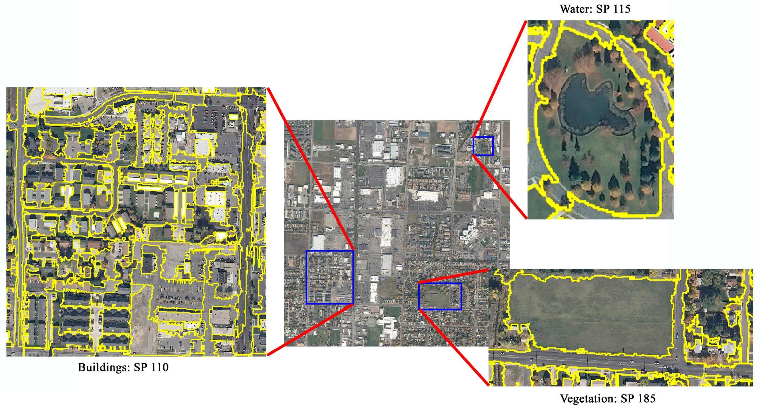
For a visual evaluation of results, we segmented the test images using the SPs identified by the RT models (as reported in Table 5), in combination with the shape/color and compactness parameters given in Table 4. It is worth noting that because the data used to construct the RT models were assumed to be pansharpened (if applicable), we also pansharpened (using the Gram-Schmidt Spectral sharpening method) the satellite images for segmentation. In Figure 4, Figure 5, Figure 6 and Figure 7, the segmentation results for different classes in four of the six test images (the 30-cm, 50-cm, 75-cm, 1-m) are depicted (for the sake of brevity, the segmentation results for the 25-cm and 65-cm test images are instead shown in Appendix B). For the 30-cm test image (Figure 4), we selected four representative land covers (i.e., building, vegetation, road, and water) to visually evaluate the performance of the respective RT models. Given the complexity of the building rooftops, the segmentation result of the buildings was generally satisfactory. However, some degree of undersegmentation occurred in areas where the rooftops had a very similar appearance to nearby non-building land covers. The vegetation class was also extracted relatively accurately, as green spaces (e.g., trees and grass) were distinguished from other land covers in most cases. The problem with green spaces in remotely sensed imagery is that their extraction could be highly scale-dependent; that is, using a single SP, it might not be possible to, for example, extract both urban forests and single trees simultaneously. This problem also occurred in this image, where trees, grass, and urban forests were all present at the same time. As a result, it can be seen that the large urban forests were oversegmented, while a few areas containing small patches of grass or single trees were undersegmented (mixed with the pixels of roads). One way to mitigate this issue could be to construct a separate RT model for each type of vegetation (e.g., one for single trees, one for tree patches, one for parks, and so on), although it may be difficult to find sufficient samples from the literature to construct these models. The results for the extraction of the roads were also generally satisfactory, having some acceptable degree of oversegmentation and no excessive undersegmentation. In general, roads could be very difficult to be appropriately extracted because of various nearby non-road features (e.g., cars, shadows, vegetation, asphalt defects, etc.) that hinder the segmentation algorithm from detecting correct boundaries of roads. The RT model established for the extraction of water bodies in this test image also performed relatively well in segmenting the pond in the image.
In the 50-cm test image (Figure 5), the accuracy of the extracted building, road, and water features was evaluated. Undersegmentation of the extracted buildings from this image was more prevalent than in the 30-cm image. One reason for this problem could be the highly spectrally similar information of some buildings to their neighboring buildings. Nevertheless, this type of undersegmentation did not cause the buildings to be mixed with other land covers. In contrast to the 30-cm test image, the roads present in the 50-cm image were not extracted properly, resulting in oversegmentation. The extraction of the small lake in this image also led to some oversegmentation, but not as much as was observed for roads.
In the 75-cm test image (Figure 6), it is evident that vegetation, road, and bare soil land cover features were extracted better than buildings and water bodies. There was again an apparent degree of oversegmentation in the extracted water bodies in this image. Moreover, some of the buildings were undersegmented, which was undesirable.
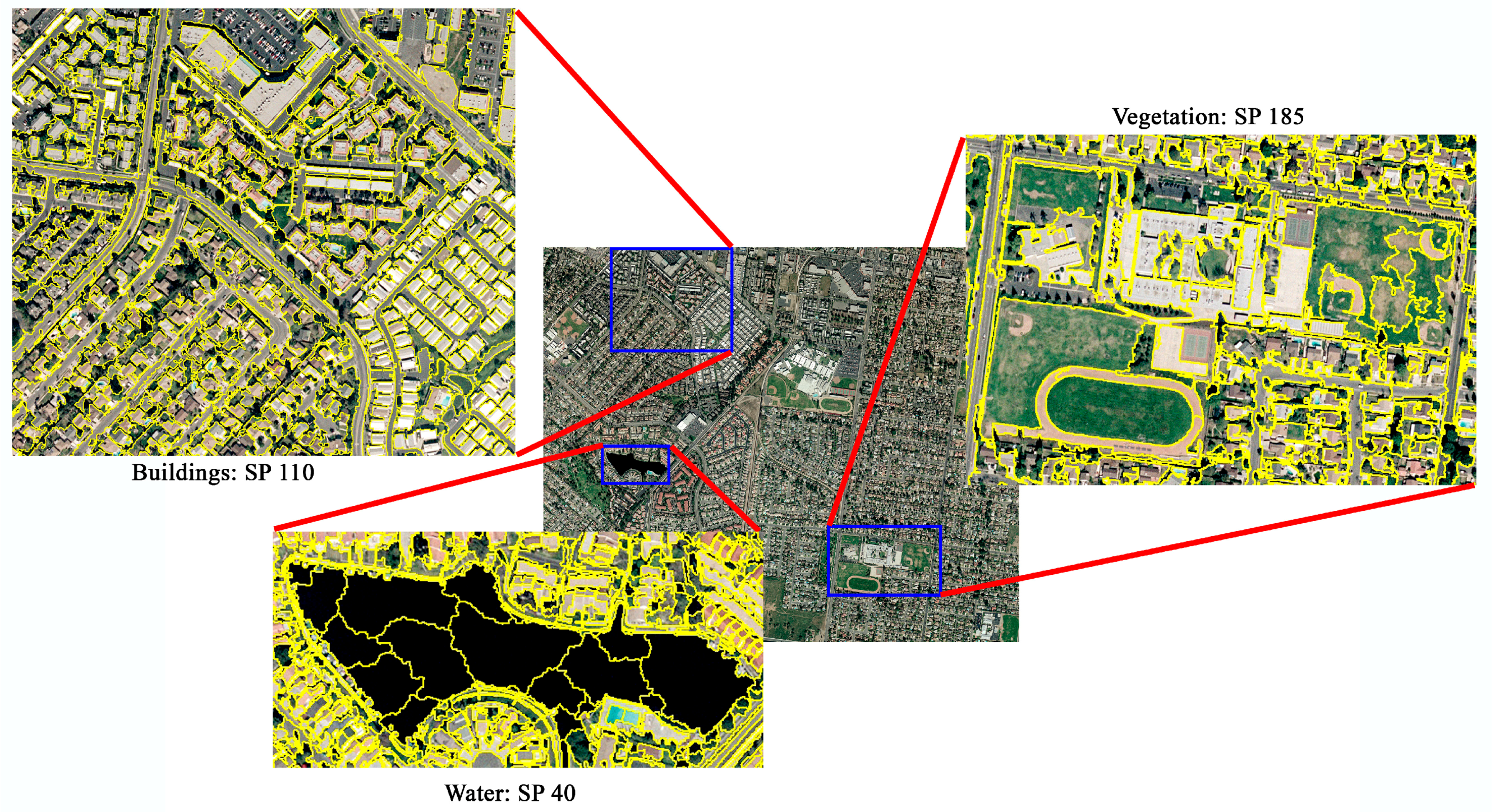
As with the segmentation results of the 50 cm and 75 cm test images, the water bodies in the 1-m image (Figure 7) were oversegmented. The buildings in this image, however, were more successfully extracted than those of the 75 cm image, although a few undersegmented buildings could be still observed. As with the results of the 30 cm image, the road class was segmented very reasonably in this test image, although there were similar spectral properties between the roads and nearby features, specifically vegetation. The vegetation land cover extracted using the SP estimated by the corresponding RT model did not generally behave consistently in this test image; that is, in some cases (e.g., over urban forests), some level of oversegmentation was apparent, but in some other cases, where the nearby buildings had similar spectral information to vegetation, undersegmentation occurred.
4.2.3. Quantitative Evaluation Results for the Test Images
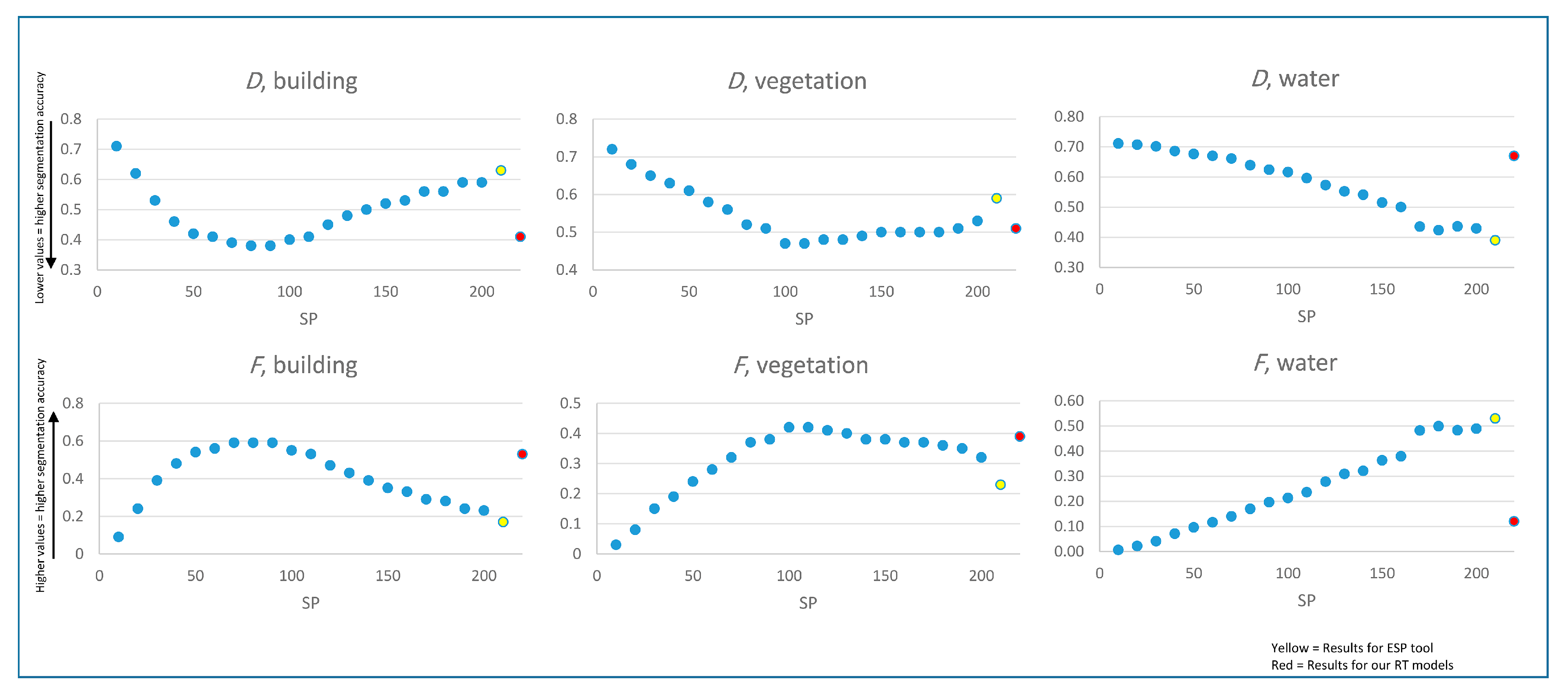
Table 6 and Figure 8 show the values of the supervised metrics calculated for the segmentations selected by our RT models for all the six test images, as well as the values for the segmentations selected by the ESP tool, and the results for a range of other segmentations. From Figure 8, it can be seen that our RT models produced more accurate segmentations than the ESP tool (lower D values and higher F values) for the building and vegetation classes, while the ESP tool performed better than our RT model for the water class. For the building and vegetation classes, our RT models also had segmentation accuracies that were among the highest of the other SPs tested, while for the water class our RT model produced less accurate segmentations than many of the other tested SPs. The main problem with our RT model predictions for the water class was likely due to the large differences in the sizes/shapes of water features extracted in the past studies, e.g., some studies aimed to accurately segment pools, others aimed to segment linear water features (rivers or canals), and yet others large water bodies (e.g., ponds or lakes). From Table 6, it is also clear that our RT models (as well as the ESP tool) resulted in more undersegmentation than oversegmentation for the building and vegetation classes, but more oversegmentation than undersegmentation for the water class. Comparing the D and F values of the RT models obtained for the building and vegetation classes, the building class was extracted more accurately, perhaps because the polygons for the vegetation class were more diverse in size and spectral heterogeneity (e.g., some polygons were of individual trees, some were larger grassy areas).
4.3. General Discussion
As the experiments in this study showed, in order to segment different land cover types successfully it is necessary to use different SPs. In other words, as already suggested in a number of studies, instead of using a single-scale segmentation approach, it is more effective to employ a multi-scale approach to extract different land cover features in a given image. Although the level of complexity of different features can vary from landscape to landscape and from image to image, thus affecting the selection of appropriate SPs, this study indicated that it is possible to narrow down the range of suitable SPs for segmenting a specific type of land cover using information from the literature and regression modeling. In previous studies, a strong emphasis was put mainly on the inverse relationship between the SP selected and the spatial resolution of an image. However, there are some other image characteristics that contribute to the selection of SPs. In this research, in contrast to many previous studies, we considered radiometric resolution of the image as another determinant of the SP estimation, although its effect on the SP was much less than that of the spatial resolution. Furthermore, the evaluation results showed that such approaches to the parametrization of SP are only a proxy for narrowing down the wide range of possible SPs to segment a given image optimally. Therefore, such an approach could significantly reduce the time and labor required to generate desirable segmentation results.
The RT models represented in this research can be applied to other urban areas as well. However, it should be noted that the RT models may fail to estimate appropriate SPs in cases where the urban structure is significantly different from those whose data were used to construct the RT models. The main cause of this problem is that the fitted RT models, which are generated using a limited number of samples, cannot completely account for all the variability encountered in the real world. One of the most viable ways through which this problem can be addressed is by increasing the amount and diversity of the data used to generate the RT models, so that they can be further generalized and better adapted to more types of urban areas. In this regard, we have provided all of the data that we used to construct the RT models in this study (provided as a Supplementary Table), so that other researchers can build upon it to achieve better results in the future (e.g., by adding more data for their classes/study areas of interest and then rerunning the RT models).
Another caveat that should be noted here is that in some studies that we reviewed and extracted details from to establish the models, a single universal SP (e.g., an SP of 10) had been used to extract all of the land covers, potentially resulting in over- or undersegmentation of some classes in these studies. This could have affected the accuracy of some of our RT models, especially for those land cover classes with small sample sizes. For instance, the oversegmented results of the water class in most of our cases demonstrate the negative effect of applying a single SP to extract multiple types of land cover present in an image. Although it is generally agreed that oversegmentation is less harmful than undersegmentation, it could still deteriorate the classification results because potentially informative non-spectral information (e.g., size and shape of land cover features) will not be utilized for training the classifier [36]. It should be hence again accentuated that the quality of a segmentation yielded in the GEOBIA framework should not be easily neglected by assigning a universal, and in most cases, very small value to the SP to extract different types of land cover in urban areas, whose complexities call for more attention in the segmentation phase.
In addition to the aforementioned problem affecting the quality of the RT models, it is important to note that the predicted SP values for the classes with lower sample sizes should be used with greater caution, and may require more fine-tuning by the user than for other classes (e.g., users may want to perform segmentation using a wider range of SP values greater/less than our identified SP value to select the most appropriate SP value for their own images).
In this study (as in many other GEOBIA studies), we have found that different land cover classes were better represented at different segmentation levels (i.e., using different SP values). However, in many cases, it is desirable to produce a multi-class land cover map (rather than separate maps of each individual land cover class). To use our approach for multi-class land cover map production, one possibility would be to perform classification in a step-wise manner (e.g., classifying the land cover types with lower SP values first, or vice versa), as has been done in several other GEOBIA studies that utilized multiple segmentation levels for classification [37,54,55,56]. More sophisticated solutions for multi-scale classification also exist (and may indeed work better than our simple example), but a deeper discussion/comparison of these methods is not provided here because it is outside the main focus of our study.
5. Conclusions
In this study, we conducted a meta-analysis to investigate the potential of employing information derived from past GEOBIA urban land cover mapping studies to select appropriate, i.e., reasonably accurate, segmentation parameters (specifically the scale parameter (SP)) for the commonly used multiresolution segmentation (MRS) algorithm. In this regard, we reviewed peer-reviewed journal papers involving GEOBIA for urban land cover mapping published from 2010 to 2017, and extracted data on the MRS parameters used, image spatial/radiometric resolutions used, and land cover types mapped, from a total number of 39 papers selected from 215 potentially relevant papers. Afterward, considering five classes (i.e., building, vegetation, road, bare soil, and water), we applied an RT model to the corresponding data of each class to predict the appropriate SP. The experiments performed on six test images (two pansharpened satellite images, and four aerial images) with different spatial resolutions (25 cm, 30 cm, 50 cm, 65 cm, 75 cm, 1 m) and with different radiometric resolutions (8 bits, 11 bits) showed that it was possible to narrow down the wide range of possible SPs that can be used to segment remotely sensed imagery for urban land cover mapping. Therefore, the RT models and equations from this study can be applied to different urban areas, although there would be no guarantee that the results would be suitable in every case. This study also confirmed the conclusions drawn by a number of other studies on GEOBIA that highlight the importance of applying a multi-scale approach to segment and extract different land cover types more accurately.
Acknowledgments
The ISPRS test imagery was made available online courtesy of Space Imaging LLC, and the aerial test images were provided online courtesy of the U.S. Geological Survey. The authors would like to be grateful to the three anonymous reviewers whose insightful comments significantly improved the quality of the paper.
Author Contributions
Brian A. Johnson conceived and designed the research. Brian A. Johnson and Shahab E. Jozdani together performed the analyses and wrote the manuscript.
Conflicts of Interest
The authors declare no conflict of interest.
Appendix A
In this appendix, the evaluation metrics used for accuracy assessment are presented. Four evaluation metrics were used in this study: OverSegmentationij (or OSegij) (Equation (A1)), UnderSegmentationij (or USegij) (Equation (A2)), D-metric (Equation (A3)), and F-measure (Equation (A4)).
In the above equations, xi is the reference polygon, yj is the segment intersecting the reference polygon xi, and area(xi ∩ yi) is the calculated area of the intersection of the reference polygon xi and the segment yj. The range of all these metrics is between 0 and 1. If the OSegij, USegij, and D-metric approach to 0, it can be concluded that an optimal segmentation result was generated. On the other hand, as the F-measure approaches 1, the quality of the segmentation results improves.
Appendix B
Figure A1.
Segmentation results of the building, vegetation, and water classes in the 25-cm test image.
Figure A1.
Segmentation results of the building, vegetation, and water classes in the 25-cm test image.

Figure A2.
Segmentation results of the building, vegetation, and water classes in the 65-cm test image.
Figure A2.
Segmentation results of the building, vegetation, and water classes in the 65-cm test image.

Appendix C
Figure A3.
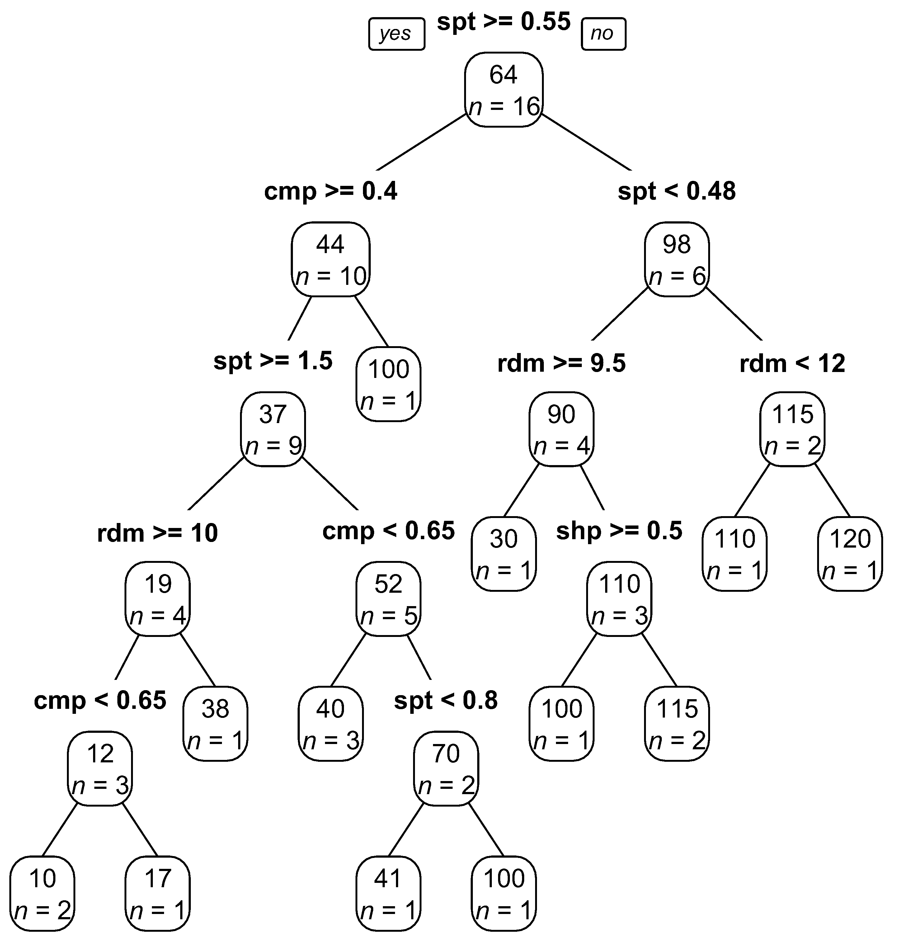
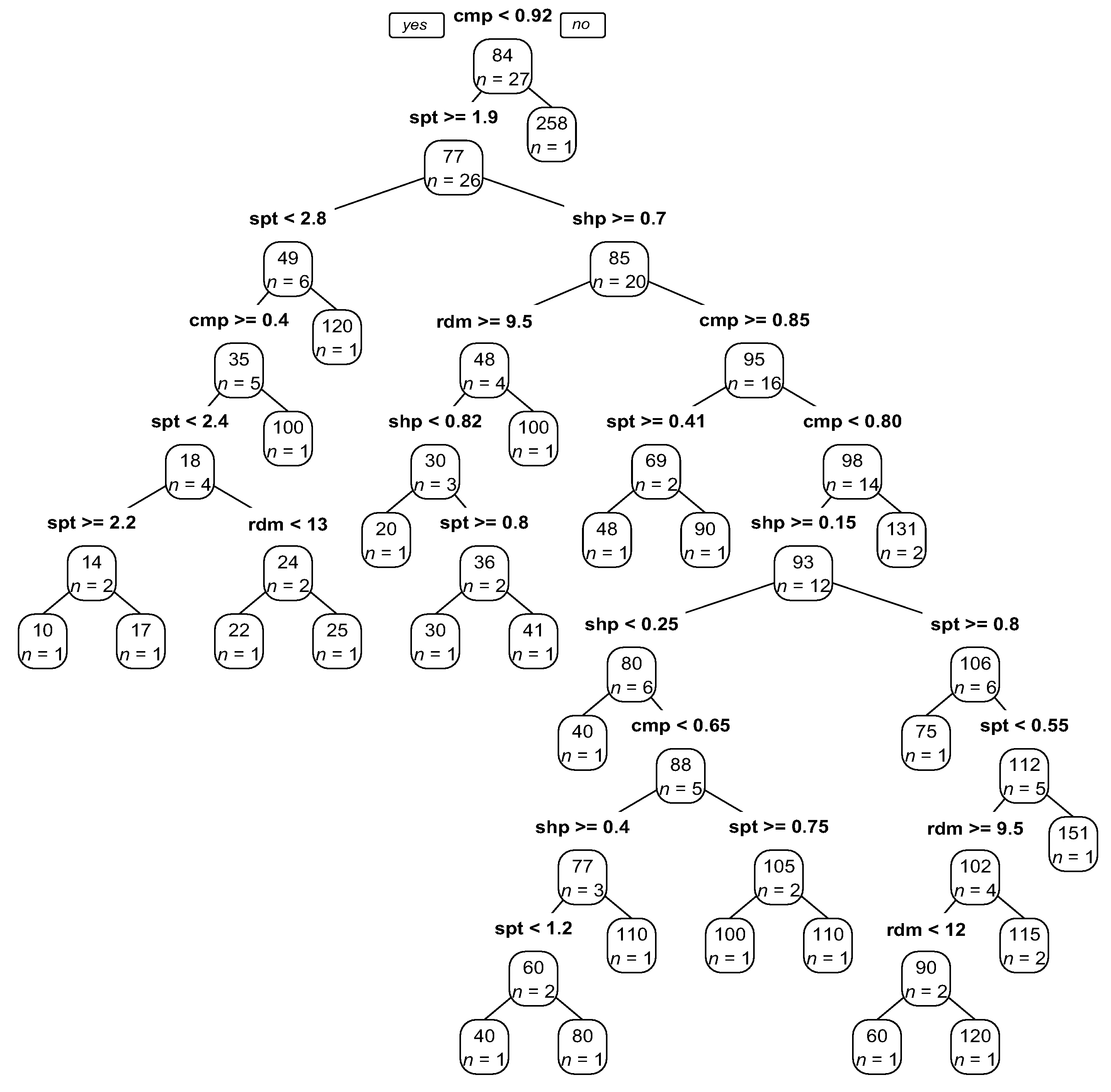
Graphical representation of the rulesets of the RT model established for the building class. Note: spt = spatial resolution, rdm = radiometric resolution, shp = shape/color weight, and cmp = compactness/smoothness weight, n = the number of samples at each node; the values in the rectangles are the estimated SPs.
Figure A3.
Graphical representation of the rulesets of the RT model established for the building class. Note: spt = spatial resolution, rdm = radiometric resolution, shp = shape/color weight, and cmp = compactness/smoothness weight, n = the number of samples at each node; the values in the rectangles are the estimated SPs.

Figure A4.
Graphical representation of the rulesets of the RT model established for the vegetation class. Note: spt = spatial resolution, rdm = radiometric resolution, shp = shape/color weight, and cmp = compactness/smoothness weight, n = the number of samples at each node; the values in the rectangles are the estimated SPs.
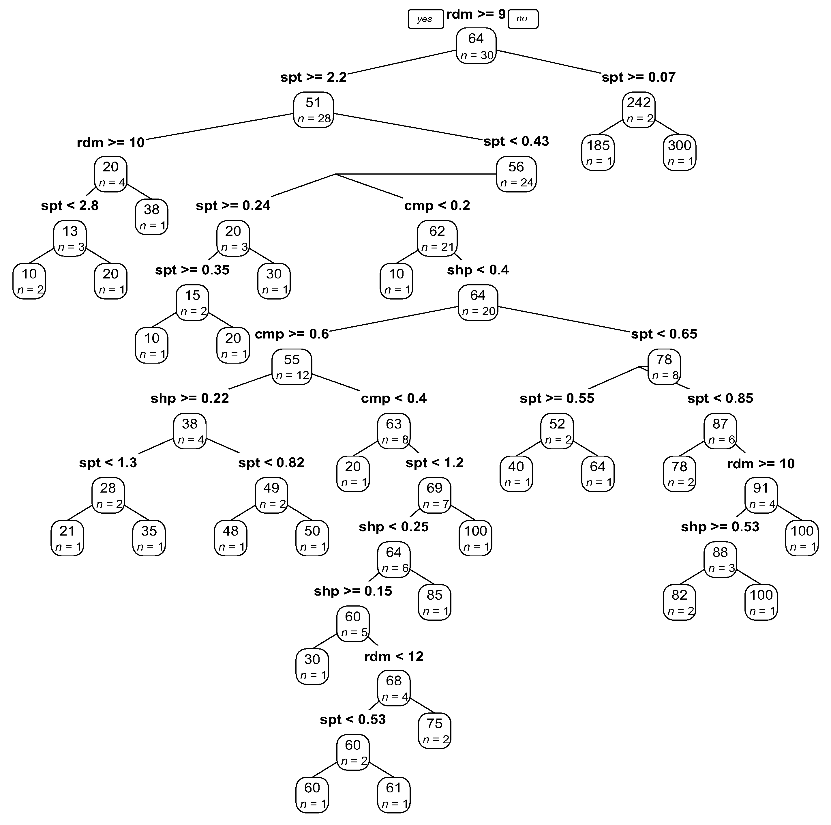
Figure A5.
Graphical representation of the rulesets of the RT model established for the road class. Note: spt = spatial resolution, rdm = radiometric resolution, shp = shape/color weight, and cmp = compactness/smoothness weight, n = the number of samples at each node; the values in the rectangles are the estimated SPs.
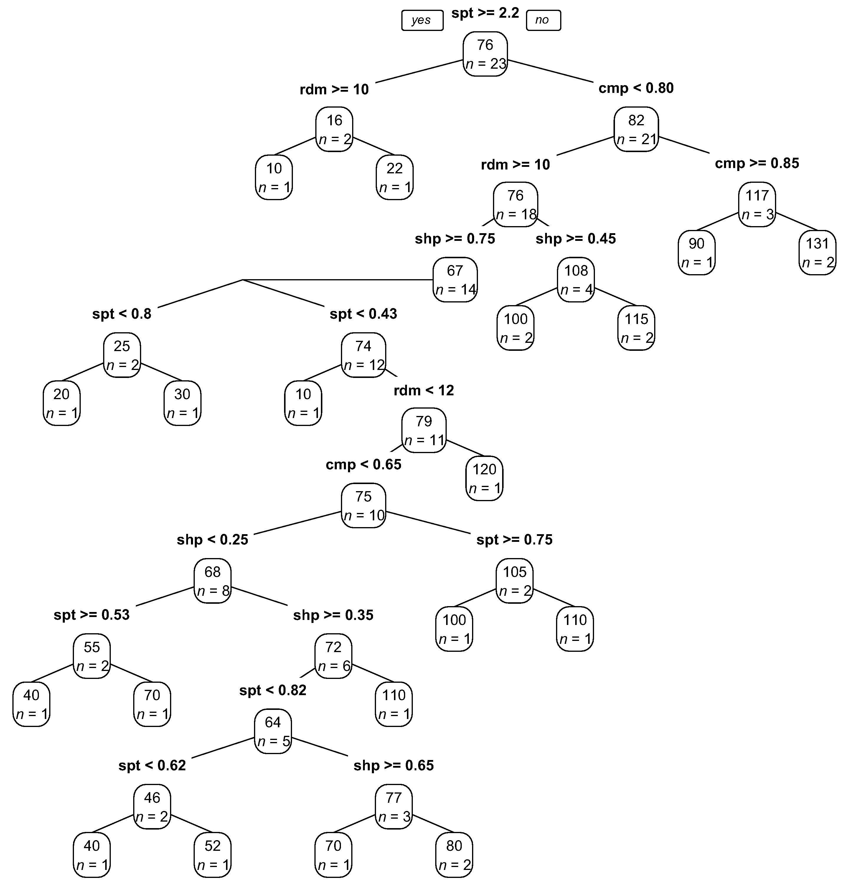
Figure A6.
Graphical representation of the rulesets of the RT model established for the bare soil class. Note: spt = spatial resolution, rdm = radiometric resolution, shp = shape/color weight, and cmp = compactness/smoothness weight, n = the number of samples at each node; the values in the rectangles are the estimated SPs.
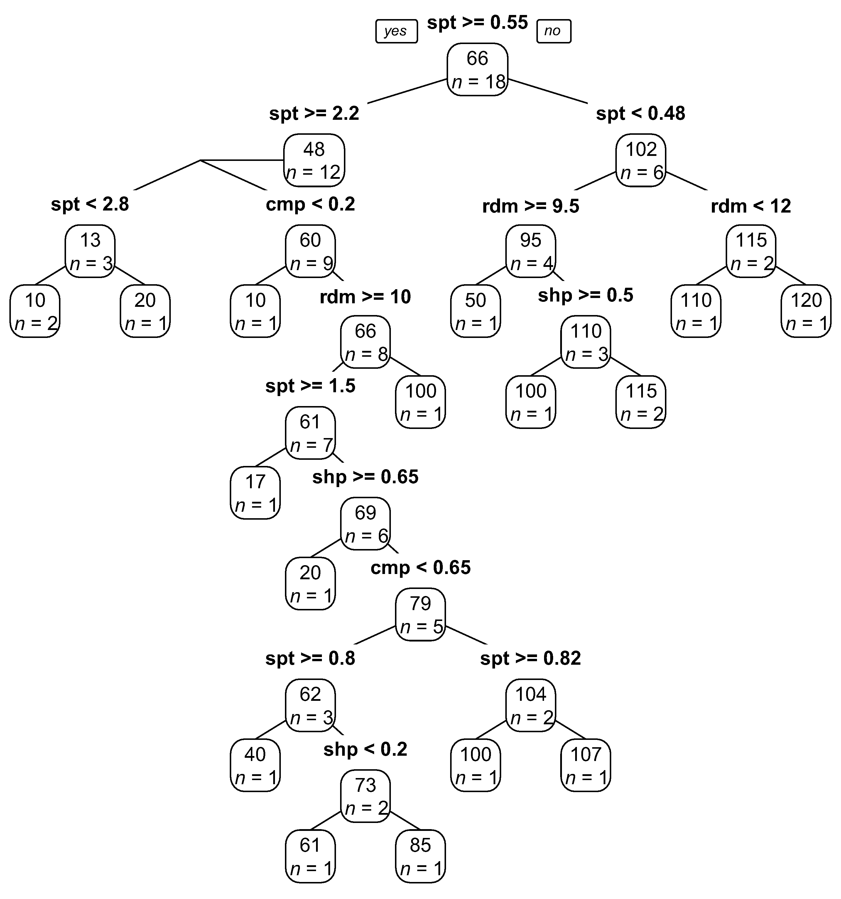
Figure A7.
Graphical representation of the rulesets of the RT model established for the water class. Note: spt = spatial resolution, rdm = radiometric resolution, shp = shape/color weight, and cmp = compactness/smoothness weight, n = the number of samples at each node; the values in the rectangles are the estimated SPs.
References
- Cetin, M. Using GIS analysis to assess urban green space in terms of accessibility: Case study in Kutahya. Int. J. Sustain. Dev. World Ecol. 2015, 22, 420–424. [Google Scholar] [CrossRef]
- Tang, Z.; Engel, B.A.; Lim, K.J.; Pijanowski, B.C.; Harbor, J. Minimizing the impact of urbanization on long term runoff. J. Am. Water Resour. Assoc. 2005, 41, 1347–1359. [Google Scholar] [CrossRef]
- Voogt, J.A.; Oke, T.R. Thermal remote sensing of urban climates. Remote Sens. Environ. 2003, 86, 370–384. [Google Scholar] [CrossRef]
- Wang, L.; Sousa, W.P.; Gong, P. Integration of object-based and pixel-based classification for mapping mangroves with IKONOS imagery. Int. J. Remote Sens. 2004, 25, 5655–5668. [Google Scholar] [CrossRef]
- Jebur, M.N.; Mohd Shafri, H.Z.; Pradhan, B.; Tehrany, M.S. Per-pixel and object-oriented classification methods for mapping urban land cover extraction using spot 5 imagery. Geocarto Int. 2014, 29, 792–806. [Google Scholar] [CrossRef]
- Platt, R.V.; Rapoza, L. An evaluation of an object-oriented paradigm for land use/land cover classification. Prof. Geogr. 2008, 60, 87–100. [Google Scholar] [CrossRef]
- Tenenbaum, D.E.; Yang, Y.; Zhou, W. A comparison of object-oriented image classification and transect sampling methods for obtaining land cover information from digital orthophotography. GISci. Remote Sens. 2011, 48, 112–129. [Google Scholar] [CrossRef]
- Jabari, S.; Zhang, Y. Very high resolution satellite image classification using fuzzy rule-based systems. Algorithms 2013, 6, 762–781. [Google Scholar] [CrossRef]
- Li, X.; Meng, Q.; Gu, X.; Jancso, T.; Yu, T.; Wang, K.; Mavromatis, S. A hybrid method combining pixel-based and object-oriented methods and its application in hungary using Chinese HJ-1 satellite images. Int. J. Remote Sens. 2013, 34, 4655–4668. [Google Scholar] [CrossRef]
- Estoque, R.C.; Murayama, Y.; Akiyama, C.M. Pixel-based and object-based classifications using high- and medium-spatial-resolution imageries in the urban and suburban landscapes. Geocarto Int. 2015, 30, 1113–1129. [Google Scholar] [CrossRef]
- Acharya, T.; Ray, A.K. Image Processing: Principles and Applications; John Wiley & Sons: Hoboken, NJ, USA, 2005; p. 428. [Google Scholar]
- Gonzalez, R.C.; Woods, R.E. Digital Image Processing, 3rd ed.; Prentice-Hall: Upper Saddle River, NJ, USA, 2007; pp. 711–800. [Google Scholar]
- Tian, J.; Chen, D.M. Optimization in multi-scale segmentation of high-resolution satellite images for artificial feature recognition. Int. J. Remote Sens. 2007, 28, 4625–4644. [Google Scholar] [CrossRef]
- Baatz, M.; Schäpe, A. Multiresolution segmentation: An optimization approach for high quality multi-scale image segmentation. In Angewandte Geographische Informationsverarbeitung XII. Beiträge zum AGIT-Symposium Salzburg 2000; Herbert Wichmann Verlag: Karlsruhe, Germany, 2000; pp. 12–23. [Google Scholar]
- Benz, U.C.; Hofmann, P.; Willhauck, G.; Lingenfelder, I.; Heynen, M. Multi-resolution, object-oriented fuzzy analysis of remote sensing data for GIS-ready information. ISPRS J. Photogramm. Remote Sens. 2004, 58, 239–258. [Google Scholar] [CrossRef]
- Witharana, C.; Civco, D.L. Optimizing multi-resolution segmentation scale using empirical methods: Exploring the sensitivity of the supervised discrepancy measure Euclidean distance 2 (ED2). ISPRS J. Photogramm. Remote Sens. 2014, 87, 108–121. [Google Scholar] [CrossRef]
- Drăguţ, L.; Csillik, O.; Eisank, C.; Tiede, D. Automated parameterisation for multi-scale image segmentation on multiple layers. ISPRS J. Photogramm. Remote Sens. 2014, 88, 119–127. [Google Scholar] [CrossRef] [PubMed]
- Johnson, B.A. Scale issues related to the accuracy assessment of land use/land cover maps produced using multi-resolution data: Comments on “the improvement of land cover classification by thermal remote sensing”. Remote Sens. 2015, 7, 8368–8390. Remote Sens. 2015, 7, 13436–13439. [Google Scholar] [CrossRef]
- Grybas, H.; Melendy, L.; Congalton, R.G. A comparison of unsupervised segmentation parameter optimization approaches using moderate- and high-resolution imagery. GISci. Remote Sens. 2017, 54, 515–533. [Google Scholar] [CrossRef]
- Jozdani, S.E.; Momeni, M.; Johnson, B.A.; Sattari, M. A regression modelling approach for optimizing segmentation scale parameters to extract buildings of different sizes. Int. J. Remote Sens. 2018, 39, 684–703. [Google Scholar] [CrossRef]
- Smith, A. Image segmentation scale parameter optimization and land cover classification using the random forest algorithm. J. Spat. Sci. 2010, 55, 69–79. [Google Scholar] [CrossRef]
- Johnson, B.; Bragais, M.; Endo, I.; Magcale-Macandog, D.; Macandog, P. Image segmentation parameter optimization considering within- and between-segment heterogeneity at multiple scale levels: Test case for mapping residential areas using landsat imagery. ISPRS Int. J. Geo-Inf. 2015, 4, 2292–2305. [Google Scholar] [CrossRef]
- Ma, L.; Cheng, L.; Li, M.; Liu, Y.; Ma, X. Training set size, scale, and features in geographic object-based image analysis of very high resolution unmanned aerial vehicle imagery. ISPRS J. Photogramm. Remote Sens. 2015, 102, 14–27. [Google Scholar] [CrossRef]
- Li, M.; Ma, L.; Blaschke, T.; Cheng, L.; Tiede, D. A systematic comparison of different object-based classification techniques using high spatial resolution imagery in agricultural environments. Int. J. Appl. Earth Obs. Geoinf. 2016, 49, 87–98. [Google Scholar] [CrossRef]
- Myint, S.W.; Galletti, C.S.; Kaplan, S.; Kim, W.K. Object vs. Pixel: A systematic evaluation in urban environments. Geocarto Int. 2013, 28, 657–678. [Google Scholar] [CrossRef]
- Li, X.; Myint, S.W.; Zhang, Y.; Galletti, C.; Zhang, X.; Turner, B.L. Object-based land-cover classification for metropolitan Phoenix, Arizona, using aerial photography. Int. J. Appl. Earth Obs. Geoinf. 2014, 33, 321–330. [Google Scholar] [CrossRef]
- Alahmadi, M.; Atkinson, P.; Martin, D. Fine spatial resolution residential land-use data for small-area population mapping: A case study in Riyadh, Saudi Arabia. Int. J. Remote Sens. 2015, 36, 4315–4331. [Google Scholar] [CrossRef]
- Drǎguţ, L.; Tiede, D.; Levick, S.R. ESP: A tool to estimate scale parameter for multiresolution image segmentation of remotely sensed data. Int. J. Geogr. Inf. Sci. 2010, 24, 859–871. [Google Scholar] [CrossRef]
- Johnson, B.; Xie, Z. Unsupervised image segmentation evaluation and refinement using a multi-scale approach. ISPRS J. Photogramm. Remote Sens. 2011, 66, 473–483. [Google Scholar] [CrossRef]
- Tong, H.; Maxwell, T.; Zhang, Y.; Dey, V. A supervised and fuzzy-based approach to determine optimal multi-resolution image segmentation parameters. Photogramm. Eng. Remote Sens. 2012, 78, 1029–1044. [Google Scholar] [CrossRef]
- Witharana, C.; Lynch, H. An object-based image analysis approach for detecting penguin guano in very high spatial resolution satellite images. Remote Sens. 2016, 8, 375. [Google Scholar] [CrossRef]
- Liu, J.; Du, M.; Mao, Z. Scale computation on high spatial resolution remotely sensed imagery multi-scale segmentation. Int. J. Remote Sens. 2017, 38, 5186–5214. [Google Scholar]
- Arvor, D.; Durieux, L.; Andrés, S.; Laporte, M.-A. Advances in geographic object-based image analysis with ontologies: A review of main contributions and limitations from a remote sensing perspective. ISPRS J. Photogramm. Remote Sens. 2013, 82, 125–137. [Google Scholar] [CrossRef]
- Belgiu, M.; Drǎguţ, L. Comparing supervised and unsupervised multiresolution segmentation approaches for extracting buildings from very high resolution imagery. ISPRS J. Photogramm. Remote Sens. 2014, 96, 67–75. [Google Scholar] [CrossRef] [PubMed]
- Ma, L.; Li, M.; Ma, X.; Cheng, L.; Du, P.; Liu, Y. A review of supervised object-based land-cover image classification. ISPRS J. Photogramm. Remote Sens. 2017, 130, 277–293. [Google Scholar] [CrossRef]
- Johnson, B.A. High-resolution urban land-cover classification using a competitive multi-scale object-based approach. Remote Sens. Lett. 2013, 4, 131–140. [Google Scholar] [CrossRef]
- Myint, S.W.; Gober, P.; Brazel, A.; Grossman-Clarke, S.; Weng, Q. Per-pixel vs. Object-based classification of urban land cover extraction using high spatial resolution imagery. Remote Sens. Environ. 2011, 115, 1145–1161. [Google Scholar] [CrossRef]
- Berger, C.; Voltersen, M.; Hese, O.; Walde, I.; Schmullius, C. Robust extraction of urban land cover information from HSR multi-spectral and LIDAR data. IEEE J. Sel. Top. Appl. Earth Obs. Remote Sens. 2013, 6, 1–16. [Google Scholar] [CrossRef]
- Cowen, D.J.; Jensen, J.R.; Bresnahan, P.J.; Ehler, G.B.; Graves, D.; Huang, X.; Wiesner, C.; Mackey, H.E. The design and implementation of an integrated geographic information system for environmental applications. Photogramm. Eng. Remote Sens. 1995, 61, 1393–1404. [Google Scholar]
- Liu, Y.; Bian, L.; Meng, Y.; Wang, H.; Zhang, S.; Yang, Y.; Shao, X.; Wang, B. Discrepancy measures for selecting optimal combination of parameter values in object-based image analysis. ISPRS J. Photogramm. Remote Sens. 2012, 68, 144–156. [Google Scholar] [CrossRef]
- Clinton, N.; Holt, A.; Scarborough, J.; Yan, L.; Gong, P. Accuracy assessment measures for object-based image segmentation goodness. Photogramm. Eng. Remote Sens. 2010, 76, 289–299. [Google Scholar] [CrossRef]
- Zhang, X.; Feng, X.; Xiao, P.; He, G.; Zhu, L. Segmentation quality evaluation using region-based precision and recall measures for remote sensing images. ISPRS J. Photogramm. Remote Sens. 2015, 102, 73–84. [Google Scholar] [CrossRef]
- Woodcock, C.E.; Strahler, A.H. The factor of scale in remote sensing. Remote Sens. Environ. 1987, 21, 311–332. [Google Scholar] [CrossRef]
- Kim, M.; Madden, M.; Warner, T. Estimation of optimal image object size for the segmentation of forest stands with multispectral IKONOS imagery. In Object-Based Image Analysis: Spatial Concepts for Knowledge-Driven Remote Sensing Applications; Blaschke, T., Lang, S., Hay, G.J., Eds.; Springer: Berlin/Heidelberg, Germany, 2008; pp. 291–307. [Google Scholar]
- Espindola, G.M.; Camara, G.; Reis, I.A.; Bins, L.S.; Monteiro, A.M. Parameter selection for region-growing image segmentation algorithms using spatial autocorrelation. Int. J. Remote Sens. 2006, 27, 3035–3040. [Google Scholar] [CrossRef]
- Gao, Y.; Mas, J.F.; Kerle, N.; Pacheco, J.A.N. Optimal region growing segmentation and its effect on classification accuracy. Int. J. Remote Sens. 2011, 32, 3747–3763. [Google Scholar] [CrossRef]
- Martha, T.R.; Kerle, N.; Westen, C.J.V.; Jetten, V.; Kumar, K.V. Segment optimization and data-driven thresholding for knowledge-based landslide detection by object-based image analysis. IEEE Trans. Geosci. Remote Sens. 2011, 49, 4928–4943. [Google Scholar] [CrossRef]
- Cánovas-García, F.; Alonso-Sarría, F. A local approach to optimize the scale parameter in multiresolution segmentation for multispectral imagery. Geocarto Int. 2015, 30, 937–961. [Google Scholar] [CrossRef]
- Yang, J.; Li, P.; He, Y. A multi-band approach to unsupervised scale parameter selection for multi-scale image segmentation. ISPRS J. Photogramm. Remote Sens. 2014, 94, 13–24. [Google Scholar] [CrossRef]
- Kruse, F.A.; Lefkoff, A.B.; Boardman, J.W.; Heidebrecht, K.B.; Shapiro, A.T.; Barloon, P.J.; Goetz, A.F.H. The spectral image processing system (SIPS)—Interactive visualization and analysis of imaging spectrometer data. Remote Sens. Environ. 1993, 44, 145–163. [Google Scholar] [CrossRef]
- Martha, T.R.; Kerle, N.; Jetten, V.; van Westen, C.J.; Kumar, K.V. Characterising spectral, spatial and morphometric properties of landslides for semi-automatic detection using object-oriented methods. Geomorphology 2010, 116, 24–36. [Google Scholar] [CrossRef]
- Stumpf, A.; Kerle, N. Object-oriented mapping of landslides using random forests. Remote Sens. Environ. 2011, 115, 2564–2577. [Google Scholar] [CrossRef]
- R Core Team, R. R: A Language and Environment for Statistical Computing; The R Foundation for Statistical Computing: Vienna, Austria, 2017. [Google Scholar]
- Kim, M.; Warner, T.A.; Madden, M.; Atkinson, D.S. Multi-scale geobia with very high spatial resolution digital aerial imagery: Scale, texture and image objects. Int. J. Remote Sens. 2011, 32, 2825–2850. [Google Scholar] [CrossRef]
- Belgiu, M.; Drǎguţ, L.; Strobl, J. Quantitative evaluation of variations in rule-based classifications of land cover in urban neighbourhoods using worldview-2 imagery. ISPRS J. Photogramm. Remote Sens. 2014, 87, 205–215. [Google Scholar] [CrossRef] [PubMed]
- Haque, M.E.; Al-Ramadan, B.; Johnson, B.A. Rule-based land cover classification from very high-resolution satellite image with multiresolution segmentation. J. Appl. Remote Sens. 2016, 10. [Google Scholar] [CrossRef]
Figure 1.
Varying spectra of different land covers over a given urban area. Note: The colors in the spectra diagrams show the distributions (histograms) of red, green, and blue bands.
Figure 1.
Varying spectra of different land covers over a given urban area. Note: The colors in the spectra diagrams show the distributions (histograms) of red, green, and blue bands.

Figure 2.
Workflow of GEOBIA framework in remote sensing.
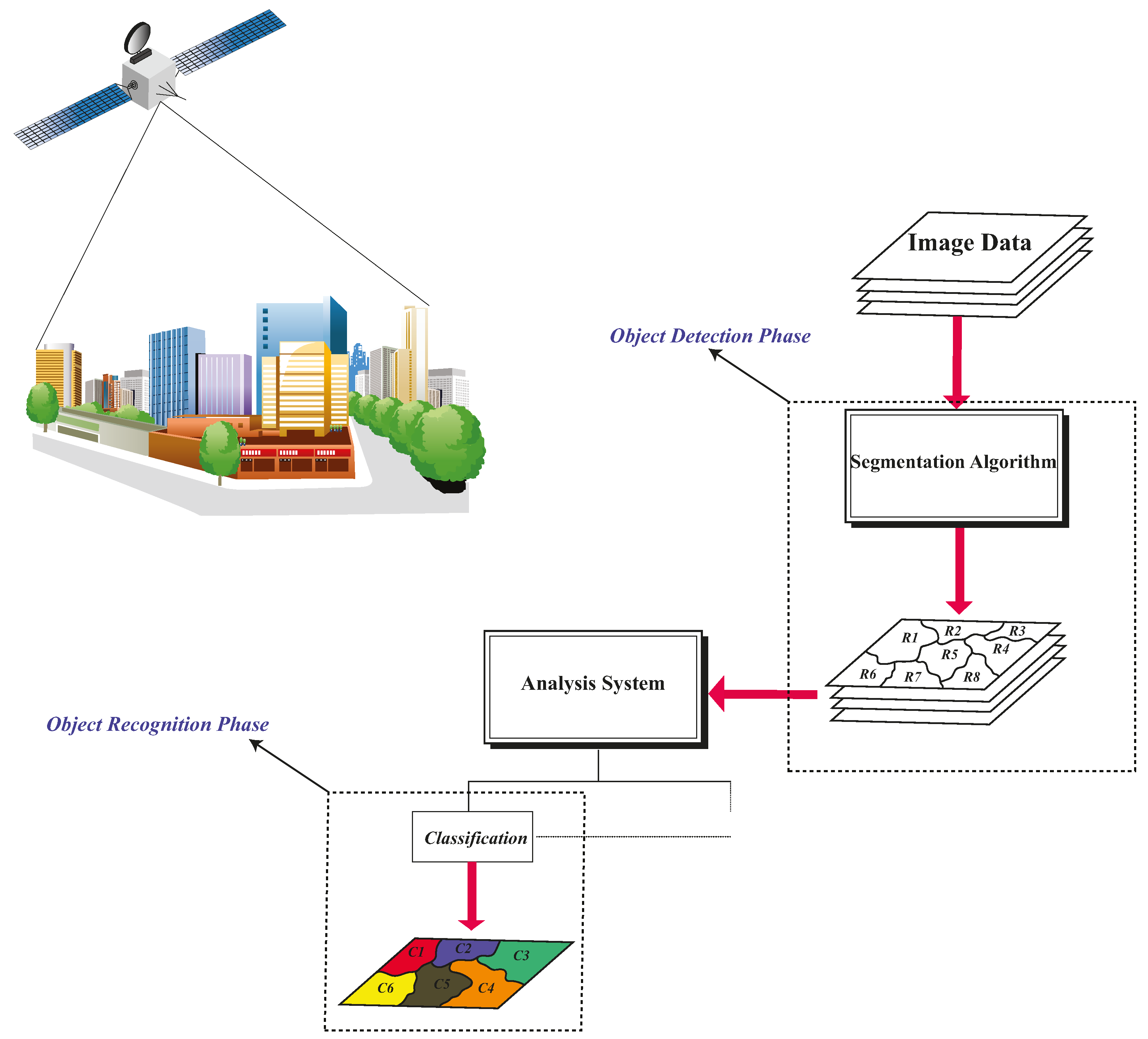
Figure 3.
Proportion of the samples data gathered from the reviewed studies for each land cover class.
Figure 3.
Proportion of the samples data gathered from the reviewed studies for each land cover class.
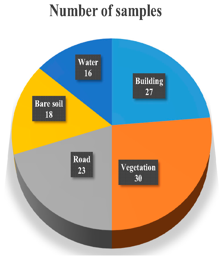
Figure 4.
Segmentation results of the building, vegetation, road, and water classes in the 30-cm test image.
Figure 4.
Segmentation results of the building, vegetation, road, and water classes in the 30-cm test image.
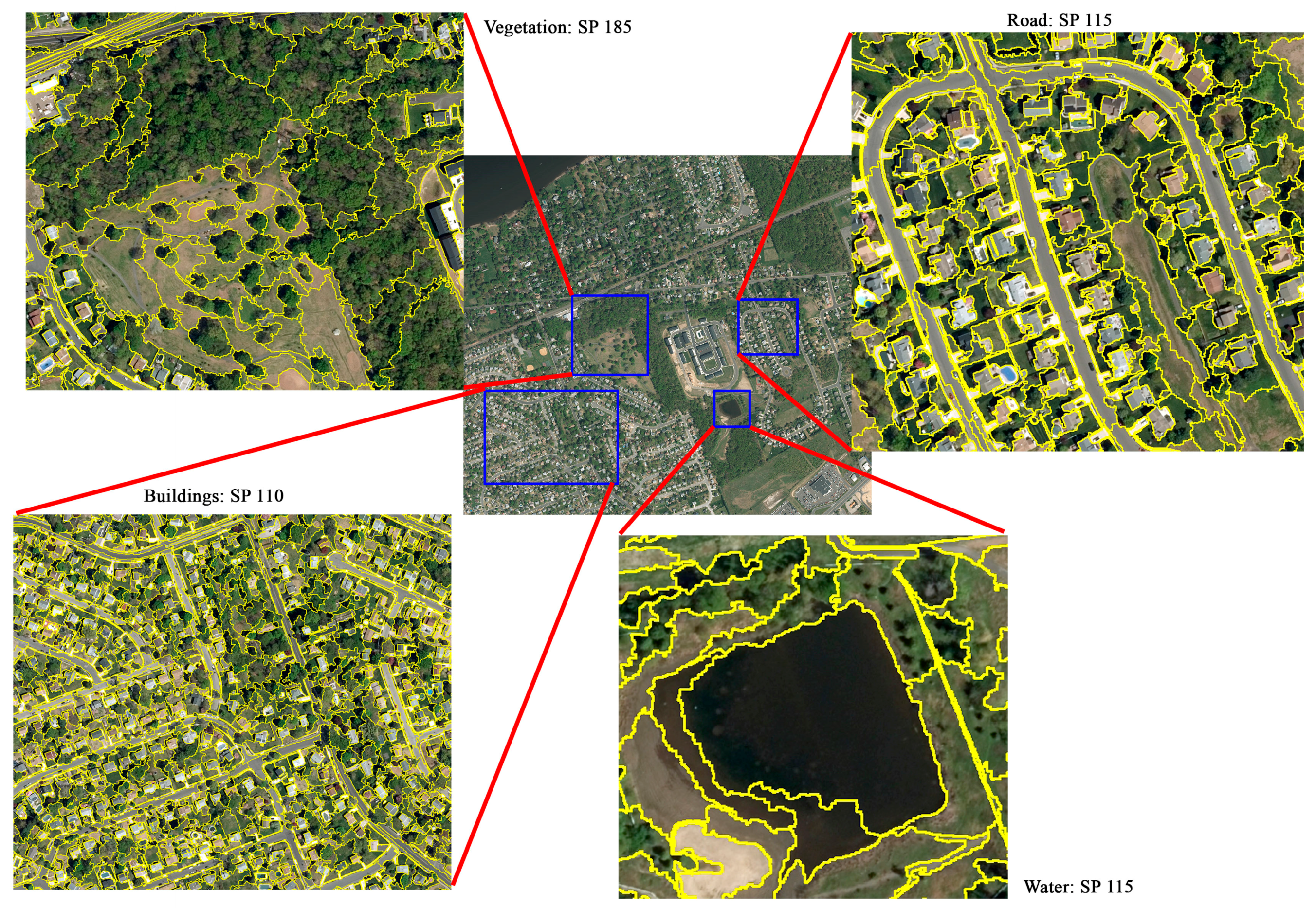
Figure 5.
Segmentation results of the building, road, and water classes in the 50-cm test image.
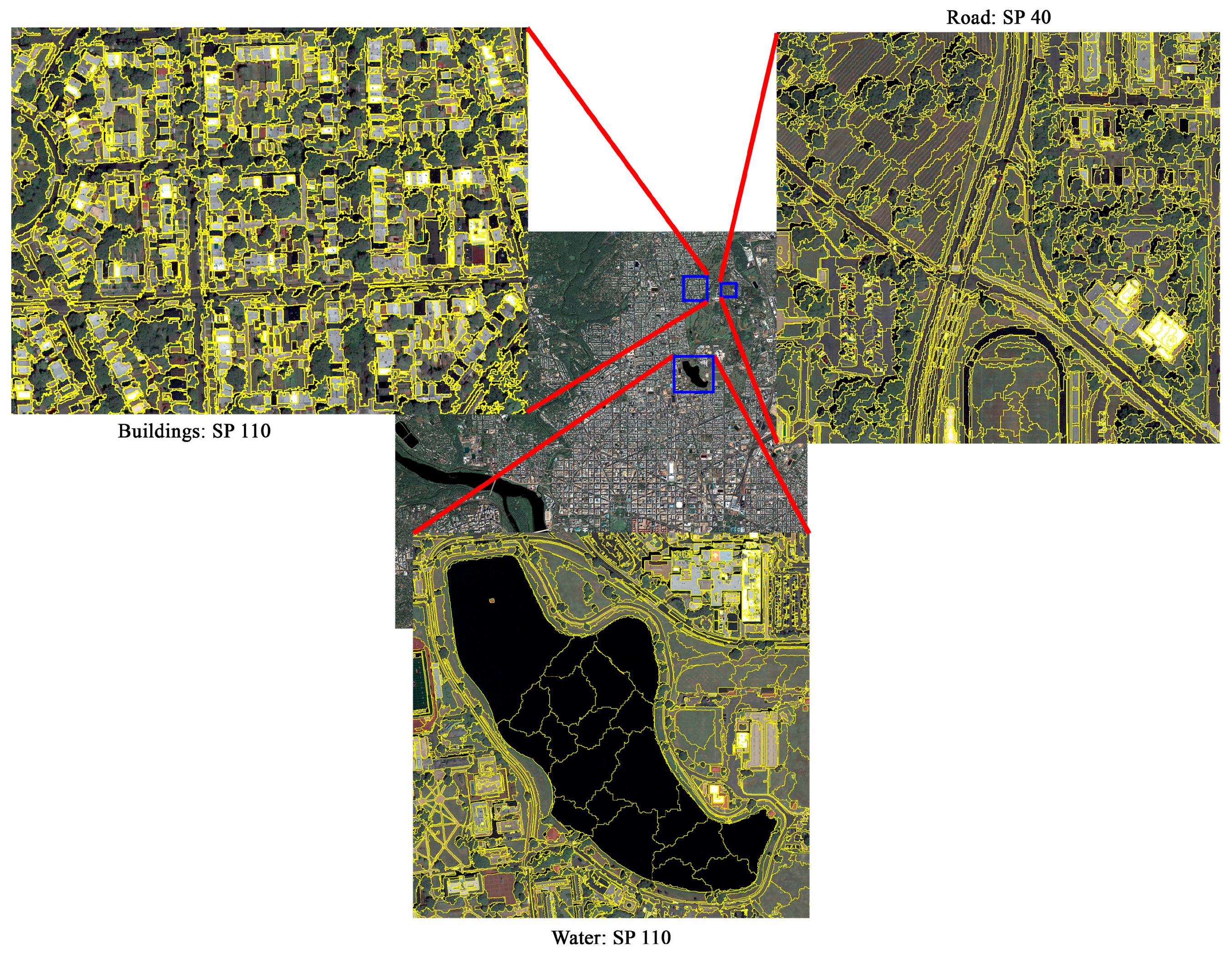
Figure 6.
Segmentation results of the building, vegetation, road, bare soil, and water classes in the 75-cm test image.
Figure 6.
Segmentation results of the building, vegetation, road, bare soil, and water classes in the 75-cm test image.
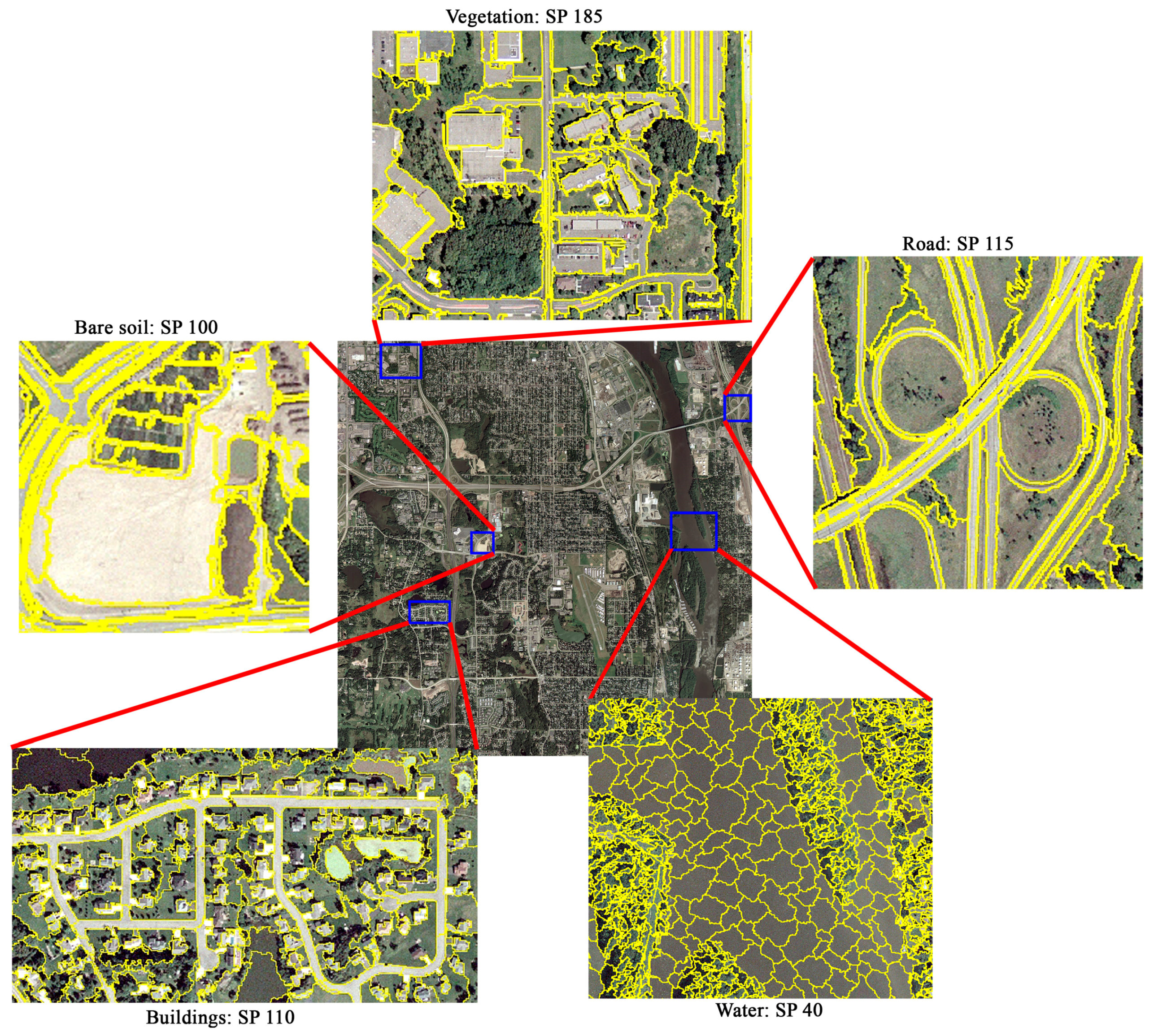
Figure 7.
Segmentation results of the building, vegetation, road, and water classes in the 1-m test image.
Figure 7.
Segmentation results of the building, vegetation, road, and water classes in the 1-m test image.
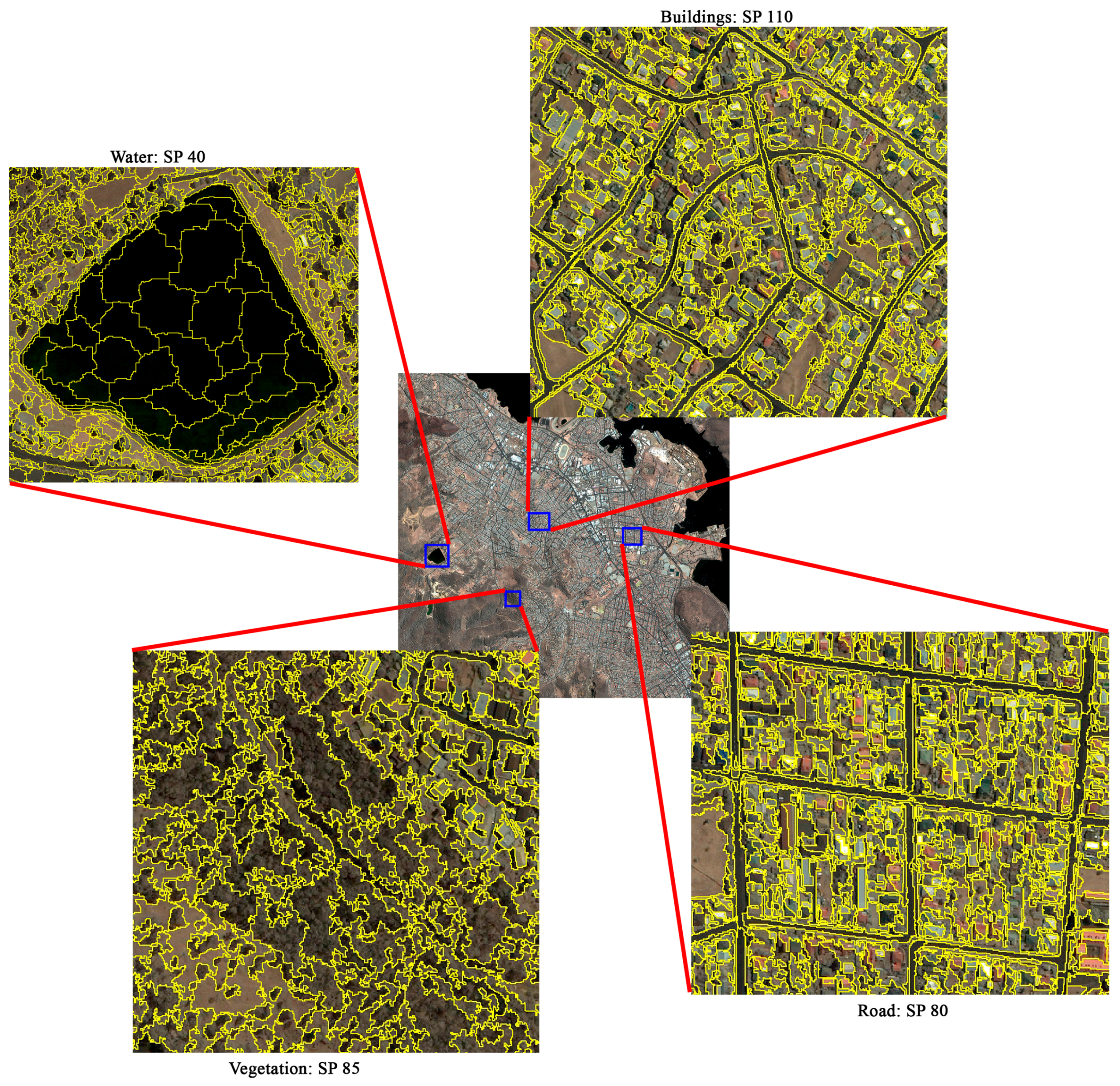
Figure 8.
Chart of the D and F values for the building, vegetation, and water classes.

Table 1.
Details of the six test images used in this study.
| Sensor | Radiometric Resolution | Spatial Resolution | Bands Used for Segmentation | Location | Tested Classes |
|---|---|---|---|---|---|
| Airborne | 8 bit | 25 cm | RGB | Cache, Utah, USA | Building, vegetation, water |
| Airborne | 8 bit | 30 cm | RGB | Calhoun, Illinois, USA | Building, vegetation, water, road |
| World-View-2 | 11 bit | 50 cm | RGB | Washington DC, USA | Buildings, road, water |
| Airborne | 8 bit | 65 cm | RGB | Riverside, California, USA | Building, vegetation, water |
| Airborne | 8 bit | 75 cm | RGB | Dakota, Minnesota, USA | Buildings, vegetation, water |
| IKONOS | 11 bit | 1 m | RGB | Hobart, Tasmania, Australia | Buildings, vegetation, road, bare soil water |
Table 2.
General information on the review process and the data extracted from reviewed papers.
| Total Number of Papers Reviewed | Number of Papers Data Extracted from | Total Number of Data | Extracted Parameters | Last Search Date |
|---|---|---|---|---|
| 215 | 39 | 114 | SP, Compactness/Smoothness, Shape/Color | 21 June 2017 |
Table 3.
Number of papers considered at each step of reviewing and reasons for eliminating papers in subsequent analyses.
Table 3.
Number of papers considered at each step of reviewing and reasons for eliminating papers in subsequent analyses.
| Step of Reviewing | Number of Papers Considered | Reason for Not Considering |
|---|---|---|
| 1 | 215 | Not related to urban mapping |
| 2 | 151 | MRS not applied |
| 3 | 124 | Optical/VHR imagery not applied |
| 4 | 88 | No classification applied |
| 5 | 39 | MRS parameters not reported |
Table 4.
Calculated mean values of the shape and compactness parameters used in the reviewed scientific papers.
Table 4.
Calculated mean values of the shape and compactness parameters used in the reviewed scientific papers.
| Class | Shape | Compactness |
|---|---|---|
| Building | 0.38 | 0.61 |
| Vegetation | 0.31 | 0.56 |
| Road | 0.44 | 0.54 |
| Bare soil | 0.36 | 0.55 |
| Water | 0.38 | 0.59 |
Table 5.
SPs estimated by the RT models for common VHR satellite sensors and the airborne sensors applied in this study. Note: the SPs were derived from the RT models based on the shape and compactness criteria defined in Table 4. The SP values are valid for pansharpened images (where applicable).
Table 5.
SPs estimated by the RT models for common VHR satellite sensors and the airborne sensors applied in this study. Note: the SPs were derived from the RT models based on the shape and compactness criteria defined in Table 4. The SP values are valid for pansharpened images (where applicable).
| Satellite/Airborne Sensor | Building | Vegetation | Road | Bare Soil | Water |
|---|---|---|---|---|---|
| IKONOS (1 m, 11 bits) | 110 | 85 | 80 | 40 | 40 |
| Quickbird (60 cm, 11 bits) | 110 | 85 | 40 | 85 | 40 |
| GeoEye-1 (41 cm, 11 bits) | 110 | 10 | 10 | 50 | 30 |
| GeoEye-2 (31 cm, 11 bits) | 110 | 20 | 10 | 50 | 30 |
| WorldView-1 and 2 (46 cm, 11 bits) | 110 | 85 | 40 | 50 | 30 |
| WorldView-3 and 4 (31 cm, 11 bits) | 110 | 20 | 10 | 50 | 30 |
| Pléiades (50 cm, 12 bits) | 110 | 85 | 120 | 120 | 120 |
| Airborne (25 cm, 8 bits) | 110 | 185 | 115 | 115 | 115 |
| Airborne (30 cm, 8 bits) | 110 | 185 | 115 | 115 | 115 |
| Airborne (65 cm, 8 bits) | 110 | 185 | 115 | 100 | 40 |
| Airborne (75 cm, 8 bits) | 110 | 185 | 115 | 100 | 40 |
Table 6.
Values of the supervised metrics calculated using all of the reference polygons for each class. The SP values used for the RT model varied by land cover class and image, and are provided in Table 3. The SP values selected by the ESP tool were: 161 (25-cm image), 236 (30-cm image), 251 (50-cm image), 266 (65-cm image), 291 (75-cm image), 271 (1-m image). Note: The parameters used for the segmentation of the test images are given in Table 4 and Table 5.
| Building | Vegetation | Water | ||||||||||
|---|---|---|---|---|---|---|---|---|---|---|---|---|
| Scale | OSeg | USeg | D | F | OSeg | USeg | D | F | OSeg | USeg | D | F |
| 10 | 0.95 | 0.18 | 0.71 | 0.09 | 0.98 | 0.10 | 0.71 | 0.04 | 1.00 | 0.04 | 0.71 | 0.01 |
| 20 | 0.83 | 0.16 | 0.62 | 0.24 | 0.91 | 0.11 | 0.66 | 0.13 | 0.99 | 0.07 | 0.71 | 0.02 |
| 30 | 0.70 | 0.17 | 0.53 | 0.38 | 0.83 | 0.18 | 0.63 | 0.21 | 0.97 | 0.10 | 0.70 | 0.04 |
| 40 | 0.58 | 0.22 | 0.48 | 0.46 | 0.73 | 0.26 | 0.60 | 0.27 | 0.95 | 0.10 | 0.69 | 0.07 |
| 50 | 0.49 | 0.27 | 0.45 | 0.51 | 0.63 | 0.33 | 0.56 | 0.33 | 0.93 | 0.12 | 0.68 | 0.10 |
| 60 | 0.42 | 0.31 | 0.43 | 0.53 | 0.56 | 0.37 | 0.55 | 0.35 | 0.92 | 0.13 | 0.67 | 0.12 |
| 70 | 0.34 | 0.35 | 0.41 | 0.55 | 0.46 | 0.45 | 0.52 | 0.38 | 0.90 | 0.16 | 0.66 | 0.14 |
| 80 | 0.24 | 0.44 | 0.41 | 0.54 | 0.36 | 0.49 | 0.50 | 0.40 | 0.86 | 0.16 | 0.64 | 0.17 |
| 90 | 0.18 | 0.49 | 0.42 | 0.51 | 0.34 | 0.51 | 0.51 | 0.39 | 0.84 | 0.16 | 0.62 | 0.20 |
| 100 | 0.13 | 0.55 | 0.43 | 0.49 | 0.25 | 0.53 | 0.48 | 0.41 | 0.82 | 0.17 | 0.62 | 0.21 |
| 110 | 0.12 | 0.59 | 0.45 | 0.46 | 0.16 | 0.60 | 0.48 | 0.41 | 0.80 | 0.17 | 0.60 | 0.24 |
| 120 | 0.11 | 0.65 | 0.49 | 0.41 | 0.14 | 0.66 | 0.51 | 0.36 | 0.75 | 0.17 | 0.57 | 0.28 |
| 130 | 0.10 | 0.68 | 0.50 | 0.38 | 0.12 | 0.67 | 0.50 | 0.36 | 0.73 | 0.18 | 0.55 | 0.31 |
| 140 | 0.09 | 0.71 | 0.52 | 0.35 | 0.10 | 0.71 | 0.53 | 0.32 | 0.70 | 0.18 | 0.54 | 0.32 |
| 150 | 0.09 | 0.73 | 0.54 | 0.32 | 0.10 | 0.71 | 0.53 | 0.32 | 0.66 | 0.19 | 0.52 | 0.36 |
| 160 | 0.07 | 0.76 | 0.55 | 0.30 | 0.09 | 0.72 | 0.53 | 0.31 | 0.64 | 0.19 | 0.50 | 0.38 |
| 170 | 0.07 | 0.79 | 0.57 | 0.27 | 0.07 | 0.74 | 0.53 | 0.31 | 0.53 | 0.21 | 0.44 | 0.48 |
| 180 | 0.07 | 0.79 | 0.57 | 0.26 | 0.07 | 0.74 | 0.54 | 0.30 | 0.51 | 0.22 | 0.42 | 0.50 |
| 190 | 0.06 | 0.82 | 0.59 | 0.23 | 0.07 | 0.77 | 0.55 | 0.28 | 0.51 | 0.23 | 0.44 | 0.48 |
| 200 | 0.05 | 0.83 | 0.60 | 0.22 | 0.07 | 0.78 | 0.56 | 0.26 | 0.48 | 0.24 | 0.43 | 0.49 |
| ESP tool | 0.03 | 0.88 | 0.63 | 0.16 | 0.07 | 0.81 | 0.59 | 0.23 | 0.30 | 0.33 | 0.39 | 0.53 |
| RT models | 0.12 | 0.58 | 0.44 | 0.47 | 0.17 | 0.69 | 0.53 | 0.34 | 0.92 | 0.15 | 0.67 | 0.12 |
© 2018 by the authors. Licensee MDPI, Basel, Switzerland. This article is an open access article distributed under the terms and conditions of the Creative Commons Attribution (CC BY) license (http://creativecommons.org/licenses/by/4.0/).
Share and Cite
MDPI and ACS Style
Johnson, B.A.; Jozdani, S.E. Identifying Generalizable Image Segmentation Parameters for Urban Land Cover Mapping through Meta-Analysis and Regression Tree Modeling. Remote Sens. 2018, 10, 73. https://doi.org/10.3390/rs10010073
AMA Style
Johnson BA, Jozdani SE. Identifying Generalizable Image Segmentation Parameters for Urban Land Cover Mapping through Meta-Analysis and Regression Tree Modeling. Remote Sensing. 2018; 10(1):73. https://doi.org/10.3390/rs10010073
Chicago/Turabian StyleJohnson, Brian A., and Shahab E. Jozdani. 2018. "Identifying Generalizable Image Segmentation Parameters for Urban Land Cover Mapping through Meta-Analysis and Regression Tree Modeling" Remote Sensing 10, no. 1: 73. https://doi.org/10.3390/rs10010073
Note that from the first issue of 2016, this journal uses article numbers instead of page numbers. See further details here.