Monitoring Water Surface and Level of a Reservoir Using Different Remote Sensing Approaches and Comparison with Dam Displacements Evaluated via GNSS

Abstract

Remote sensing allowed monitoring the reservoir water level by estimating its surface extension. Surface extension has been estimated using different approaches, employing both optical (Landsat 5 TM, Landsat 7 ETM+ SLC-Off, Landsat 8 OLI-TIRS and ASTER images) and Synthetic Aperture Radar (SAR) images (Cosmo SkyMed and TerraSAR-X). Images were characterized by different acquisition modes, geometric and spectral resolutions, allowing the evaluation of alternative and/or complementary techniques. For each kind of image, two techniques have been tested: The first based on an unsupervised classification and suitable to automate the process, the second based on visual matching with contour lines with the aim of fully exploiting the dataset. Their performances were evaluated by comparison with water levels measured in situ (r² = 0.97 using the unsupervised classification, r² = 0.95 using visual matching) demonstrating that both techniques are suitable to quantify reservoir surface extension. However ~90% of available images were analyzed using the visual matching method, and just 37 images out of 58 using the other method. The evaluation of the water level from the water surface, using both techniques, could be easily extended to un-gauged reservoirs to manage the variations of the levels during normal operation. In addition, during the period of investigation, the use of Global Navigation Satellite System (GNSS) allowed the estimation of dam displacements. The advantage of using as reference a GNSS permanent station positioned relatively far from the dam, allowed the exclusion of any interaction with the site deformations. By comparing results from both techniques, relationships between the orthogonal displacement component via GNSS, estimated water levels via remote sensing and in situ measurements were investigated. During periods of changing water level (April 2011–September 2011 and October 2011–March 2012), the moving average of displacement time series (middle section on the dam crest) shows a range of variability of ±2 mm. The dam deformation versus reservoir water level behavior differs during the reservoir emptying and filling periods indicating a hysteresis-kind loop.

1. State of Art and Introduction

Real-time monitoring and protection of strategic structures such as dams are necessary since these have social, economic, and environmental importance. The evaluation of the coherence between expected displacements and water levels over time could reveal whether the structure may suffer damages, a signifier that eventually could indicate a compromised safety expectation. In this way it would be possible to ensure proper functionality of a dam and its durability over time, rectifying any potential structural deficiency.

GNSS monitoring systems, used in combination with geotechnical, hydraulic and structural systems could allow the monitoring of real-time dam displacements, with high accuracy, even remotely. In several countries GNSS technology is used to monitor complex structures, including dams [1,2,3].

Among these cases, an integrated system has been set [4] to monitor the effects of water loads over three earthen dams near Hemet, United States of America (USA), which represent the largest water storage in the south of California. In particular, geotechnical instrumentation, active Continuously Operating Reference Station (CORS) GNSS and a fully automated terrestrial geodetic system were set up to evaluate the displacements of control points located on the crest and downstream sides of the dam within a tolerance of 10 mm at 95% confidence level.

Following an earthquake affecting the Sermo Dam in the Java Island (Indonesia), deformations were evaluated [5] using fixed multi-sensors (3D robotic total station, CORS sensors, automatic water level recorders, and digital IP cameras) and prisms. A base and a back sight station were located to analyze both dam displacements and stability of the surrounding area. The “reference” base station was positioned on a nearby tower proposed to be unaffected by the dam deformation. Water load also influences the state of a dam, thus, the knowledge of actual and expected deformations could point out any anomaly causing an eventual failure of a structure. Thus, many authors focused their research on assessing direct relationships between ordinary dam displacements and water levels.

Several studies were performed on Turkish dams with different approaches. A conventional geodetic monitoring system and a dynamic model were used to monitor the Yamula Dam. In particular, the vertical and horizontal displacements of many points distributed on the structure, were monitored through a geodetic positioning system during the first filling period. A dynamic model, resulting from measured displacements and water level, revealed maxima displacements at the center of the dam, and an apparent linear relationship between the changing reservoir level and the ordinary deformations of the dam [6]. The deformations of Ataturk dam were evaluated by monitoring several Global Positioning System (GPS) control points. The largest displacements were found on the upstream part of the crest and they were both horizontal and radial. Even though GPS and traditional measurements showed a comparable accuracy (<±1 cm), the study highlighted a non-perfect correlation between radial displacements and reservoir water level [7]. Finally, the horizontal displacements during the first filling period of the Ermenek Dam were analyzed using a geodetic network with total station and prisms. The orthogonal and tangential horizontal components showed a periodic behavior, with a linear trend related to temperature seasonal fluctuations of the concrete and increasing linearly with water level [8].

Besides the influence of water loads on the dam displacements, it also became important to investigate the water level change during the different emptying and filling period. Among the techniques that, in recent years, allow the recording of the reservoir water level, the authors focused their attention on the indirect estimation via remote sensing, since it is also applicable where in situ data is unavailable. Other authors [9] classified Moderate Resolution Imaging Spectroradiometer (MODIS) 16-day 250 m vegetation index products to obtain time-series, virtually cloud free, of water storage for 34 large reservoirs in the USA. The elevation-area relationship was derived, to obtain either the surface area or the water elevation when direct observations were unavailable, using altimetry products. Despite the low spatial resolution of these images and the possibility of cloud cover, the advantage of using these products is their high temporal revisit time (twice a day during diurnal hours). Higher spatial resolution optical images, such as those acquired by the Landsat mission, allow a more detailed evaluation of the surface water extent, although on the other hand, they are susceptible to cloud cover. SAR images try to exceed this limit allowing the identification of water bodies’ extension under cloudy, rainy, lacustrine foggy conditions as well as in the darkness (active sensor). For example, small reservoirs (surfaces <900 m²) were monitored using TerraSAR-X StripMap images (HH polarization) [10]. Indeed, the wavelength characterizing the TerraSAR X-band penetrates through clouds and thus, it is operational under almost all weather conditions. The surface-volume-depth relationship of the Urmia Lake, was calibrated through radar altimetry and high-resolution optical images [11].

Although radar altimetry has been designed for ocean applications and it is evident that calibration over oceans does not apply to inland seas, it has been widely applied to monitor inland waters. Some authors [12] calibrated/validated the Envisat satellite radar altimeter over Lake Issykkul (Kyrgyzstan). However, over inland water bodies, this technique is constrained by several factors (e.g., corrections, re-tracking, geographical effects). Other effects have been highlighted in previous studies [13]. Moreover, altimetry data for inland lakes are neither available readymade, nor is the extraction straightforward. The Envisat mission terminated on April 2012, after the loss of contact with the satellite, however, data was generated with nominal along-track spatial separation of ~400 m, thus few pure water signals could originate from small lakes characterized by a surface of ~ 1 km². All these factors limit the monitoring to larger inland bodies.

Recently, a rock dam was monitored trough Differential SAR Interferometry (DInSAR) and GNSS in the Taiho Subdam (Japan), showing strong correlation (r = −0.8) using either the ascending or descending orbits [14]. The advanced permanent scatterers InSAR technique, allowed evaluating the rate of continuous non-linear deformations of a dam over time caused (among factors) by variable water level [15].

Both remote sensing and GNSS techniques are helpful where data is unavailable, or where it is not feasible to retrieve data elsewhere.

This study analyses the advantages and disadvantages of different optical and SAR remote sensing methods to estimate water surface and level over a whole emptying and filling period of a reservoir. Results were compared with GNSS displacements to evaluate any relation between the variables.

As a first approach, a dataset from a short GNSS monitoring period (about three months) was analyzed, as was optical remote sensing for water surface detection. A good determination coefficient (r²) was found ranging between 0.5 and 0.7 [16].

Recently, the displacements of the dam were investigated using hydraulic and geotechnical models, and using GNSS. GNSS time series were compared with in situ conventional geodetic measures (total station and digital level). While differences were of few millimeters for the planimetric components, the time series appears scattered for vertical GNSS components. Indeed, the accuracy of GNSS data are in a range of ±10 mm, while the accuracy of spirit leveling allowed to obtain better results for vertical deformations [17]. Based on these preliminary studies, displacements were monitored over two years and water levels were investigated for a longer period than that closely related to the displacement monitoring (08 April 2011–13 May 2013), using satellite images from 22 January 2011 to 29 July 2013. The satellite dataset included different types of imagery (both optical and SAR) to investigate the relationship between the variables during both an emptying and filling period of the reservoir.

2. Theory and Methods

After reporting radiometric calibrations applied to optical and SAR remote sensing images, two methods for the determination of the water level were tested to ascertain the benefits and disadvantages if applied on images with different radiometric and geometric properties (optical and SAR) and the GNSS data processing to derive dam displacements subsequently stated.

2.1. Radiometric Calibration of Remote Sensing Data

Landsat 5 (LS5), Landsat 7 (LS7), Landsat 8 (LS8) and Advanced Spaceborne Thermal Emission and Reflection Radiometer (ASTER) optical images, and TerraSAR-X (TSX) and Cosmo-SkyMed (CSK) radar images were analyzed. The Landsat and ASTER images were obtained from United States Geological Survey (USGS) EarthExplorer portal (https://earthexplorer.usgs.gov). The ASTER images are characterized by three bands in the Visible and Near InfraRed (VNIR), five bands in the Thermal InfraRed (TIR) and six bands in the ShortWave InfraRed (SWIR). Due to geometric (or spatial) resolution (R_G), only VNIR bands were processed. LS7 and LS8 images consist of multispectral and thermal bands, and a panchromatic band with higher spatial resolution. Images of the LS7 archive are characterized by the permanent failure of Scan Line Corrector (SLC) starting from 31 May 2003. The effect of SLC-Off is prominent along the edge of the scene and gradually diminishes toward the center of the scene, which contains very little or no data loss, while the maximum width of the data gaps occurs along the edge of the image. The width of missing scan lines varies with position within the scene. Preliminarily, optical images were calibrated in spectral radiance [18] and reflectance [19], while SAR images were calibrated in brightness and backscattering (see [20,21] for TSX and CSK radiometric calibrations, respectively). However, SAR images are characterized by speckle noise, which, among several techniques, can be minimized by preliminarily aggregating brightness pixels. The pixel aggregate resampling method averages all of the pixel brightness values that contribute to the output pixel.

A flow diagram (Figure 1) summarizes the processing of both optical and radar images.

A similar approach was used to evaluate whether average resolution optical images (e.g., Landsat) and those radiometrically enhanced (e.g., using resolution merge) are suitable to estimate water surface extension with tolerable loss of accuracy. To this end, a small, an average and a large Sicilian reservoir were selected. The water surface of these reservoirs at the acquisition time was taken as reference extension, S_i. Over these areas, high-resolution satellite images were aggregated at decreasing spatial resolution aiming to quantify the loss of accuracy when estimating the water surface at lower spatial resolution, S. The loss of accuracy was quantified by calculating the relative variation of the surface estimates, $\Delta S=\left(S-S_i\right)/S_i$, with varying R_G. Aggregation levels were set to multiples of original spatial resolution.

Once the average resolution optical images were demonstrated suitable for analysis, two techniques were tested to evaluate the reservoir surface and water level: (i) The first is based on the visual matching of the water boundaries with the contour lines; (ii) the second quantifies the water surfaces by classification, then water level is retrieved, applying the relationship between water surface and storage characterizing the reservoir.

2.1.1. Pixel Aggregate on SAR Images

To evaluate if the loss of spatial resolution influences the accuracy in the determination of the water surface, preliminarily brightness pixels were aggregated to lower spatial resolution. The pixel aggregate resampling method averages all of the pixel values that contribute to the output pixel. The contribution of each input pixel to the output pixels is a weighted average based on the contributing area of each pixel to the output pixel area; when the resampled resolution is a multiple of the raw R_G (and that is the case for the present analysis) it coincides with the straight average. Thus, an analysis is required to determine the level of aggregation that maximizes the accuracy of the water surface estimation.

Next sections report visual matching and classification techniques. Both were applied on optical and SAR imagery.

2.1.2. Visual Matching

The detail of the extracted shoreline over optical images can be improved by applying a resolution merge (RM) technique, while a more suitable band combination was chosen to enhance the discrimination between land and water.

The false-color composition most suitable to identify the contour line matching the water bounds from LS5, LS7 and LS8 is given by SWIR and Near Infrared (NIR) bands, while from ASTER images is given by VNIR bands. The choice of NIR and SWIR bands, when available, is due to the bottom radiance contributing to determine the emerging radiance through the diffuse attenuation coefficient, K_d. Indeed, the higher K_d the lower bottom radiance emerging from the water surface [22]. Since K_d decreases with wavelength, NIR and SWIR spectral bands are more suitable to discriminate shallow water from land through a false-color visualization. Single-band single-polarization SAR images (both CSK and TSX) allow only grey-scale visualization. LS7 and LS8 images have a panchromatic (PAN) band characterized by higher spatial resolution than multispectral (MS) bands. MS bands were combined with PAN using RM technique based on the Principal Component (PC) analysis [23] to increase the spatial details of the water bounds, minimizing the distortion of the radiometric information.

Although the RM histograms closely match those of the MS image, shadows details in the PAN image cause distortions in the output RM image.

Water levels were weighted between the left and right bank estimates by visually matching the water bounds with the contour lines. Since the lower the slope, the more accurate the planimetric assessment, weights were assumed to be inversely proportional to the banks’ slopes depending on the geo-referencing correctness.

To analyze the accuracy of the visual matching technique, we calculated the water level range of variability ($\Delta$H), associated with different image resolutions for the given average slope of the two banks.

Water boundaries cannot be easily distinguished over a mixed pixel while pure water pixels are easily recognizable using both NIR and X-band images. Thus, it is important to select the optimum band combination. The coherence between water levels obtained by visual matching (H_e) with levels recorded in situ (H_m) depends mainly on two image characteristics: Primarily, on planimetric positioning accuracy, and secondly, on geometric resolution. Although all images were provided in World Geodetic System 1984 (WGS84), in many cases additional fine geo-referencing was required to improve matching with the contour lines. Results were compared with the water levels measured in situ.

2.1.3. Classification

The other technique is based on a classification process to assess the water reservoir extension and then the water level.

While both supervised and unsupervised image classification algorithms could have been utilized, unsupervised classification precludes operator subjectivity during automation. The K-means classification requires some parameters to be set including the number of classes, change threshold, and maximum number of iterations.

The latter was used for the analysis, through which the clusters are defined iteratively with a clustering algorithm. At each iteration, the algorithm recalculates class means and clusterizes the pixels. The process continues until the number of pixels in each class changes by less than the change threshold, or the maximum number of iterations is reached [24]. In particular, three classes were used for the reservoir classification, setting a maximum number of 100 iterations and 1% change threshold. The identified classes are water, bare soil and vegetated soil.

The use of LS7 ETM+ SLC-Off scenes strengthened the time series. Different methods exist in literature based on a moving window and local linear histogram to fill the gaps prior to classification. Gap filling was practically mandatory for subsequent classification in order to detect the reservoir surface using LS7. For the purposes of this research, the RSI ENVI 4.3 “replace bad values” (RBV) method was used. This technique fills the missing values based on Delaunay triangulation, with triangles calculated from the surrounding values.

For the other optical images, the K-means classification was applied on all VNIR bands (for ASTER images) and SWIR bands (for Landsat).

After the unsupervised classification, two different post-classification techniques were used [25]. The first one, applied to the whole dataset, is a segmentation technique, which converts a classified image into an image of connected regions in a given class thus allowing the identification of only the pixels belonging to the reservoir surface.

The minimum number of pixels required for a region to be defined as a segment, called population minimum, was set as 1000; for the connectivity, four neighboring pixels were used, with the exception of two CSK images for which the number of neighboring pixels was set as 8.

The chosen area of interest was a rectangle strictly limited to including the lake surface at its maximum water level during the monitoring period. SAR images were aggregated at lower resolution to minimize the speckle effect; however, residual speckle reduces the classification performance.

The CSK images are characterized by a surface roughness that could be due to wind action. Generally, the water surface under calm conditions reflects the radar signal away from the sensor; as a consequence, the backscatter signal which returns to the sensor is low and the water surface manifests as dark. The wind action produces waves and ripples, resulting in the radar signal being backscattered towards the sensor, producing brighter water surfaces [26]. The authors report that the variability of the backscatter between the water surface and the land should be related to the wind speed, direction and the distance over which it blows (fetch), and to the varying morphology that could influence the detection of reservoir surfaces during the classification process. Under calm conditions, for HH bands, the water surface appears dark in the radar image, while under windy conditions, the rough water surface appears bright. Front of capillary waves are induced by the orthogonal wind direction, thus, the higher the wind speed in the look direction, the higher the backscattering. For all CSK images, the correspondence between the hourly average wind direction and speed, and look direction of the scene acquisition was verified. The two CSK images in which the surface shows evident roughness have an average wind speed greater than 1.5 ms⁻¹ in the hours antecedent to acquisition, and a speed direction (at 2 m height) aligned with the look direction. The wind data was recorded from a weather station (Bivona, 37°35’43’’N, 13°24’55’’E, WGS84), located at a distance of ≈2 km north direction of the dam.

The other post-classification technique, used only for SAR images, was the class clumping, using morphological operators, to add spatial coherency to existing classified areas affected by speckle or holes, using a kernel with a specific size (3 × 3 for this study).

Results from the two methods were compared with in situ measures. Statistics were used to quantify the relationship between evaluated water levels and in situ measurements.

2.2. GNSS Processing

Previous work showed that the accuracy that can be achieved through a network of permanent stations is suitable to monitor displacements of a structure [16]. The coordinates of the permanent stations used for the monitoring refer to the terrestrial reference system (TRS). A Terrestrial Reference frame provides a set of coordinates of points located on the Earth’s surface. There are several variable global reference systems, referring to global or local frames. Among these, the International Terrestrial Reference System (ITRS) provides a world spatial reference system co-rotating with the Earth through its diurnal motion in space. The reference stations coordinates were computed in International GNSS Service, epoch 2008.0 (IGS08) system.

GNSS data was post-processed using the software Network Deformation Analysis (NDA) Professional. The software applies simplified tropospheric corrections involving the Saastamoinen and Niell mapping functions [27,28], while the ionospheric error was determined according to the Klobuchar model [29]. The software also applies ocean loading corrections based on Schwiderski’s model [30]. NDA was applied successfully in several applications (e.g., [31,32]) allowing similar accuracy than Bernese software [33,34].

A single baseline was used for the connection between the GNSS receiver and the permanent station. The displacement components were referred to the permanent station of Agrigento (AGRI). The choice of AGRI permanent station arises from a preliminary study [16], in which the time series processing has been derived from single baselines connected to four permanent stations (AGRI), Prizzi (PRIZ), Palermo (PALE), Trapani (TRAP) belonging to the UNIPA CORS network [35]. Best estimates were obtained from AGRI station.

For the baseline processing, the zenith troposphere estimation (affecting the baseline coordinates estimation) was enabled on both reference and rover stations (recommended for baseline over 15 km). According to the multi-frequency strategy, double-differenced observation data coming from the L5 (wide-lane) and L3 (ionospheric-free) frequency combination was used. This option is recommended for baseline length greater than 10 km by the software. To correct the error related to the satellite orbit, precise ephemeris (sp3 format) were used, while for the correction of the antenna phase center position, which is variable with the frequency and the elevation of the GNSS satellites, parameters provided by the International GNSS Service (IGS) were employed. The main parameters used are the time range (30 s), cut-off angle (10°), receivers for measurements of code and phase with double frequency using the double constellation of GPS and Globalnaya Navigazionnaya Sputnikovaya Sistema (GLONASS) satellites. Additional parameters used for the analysis are the rotation parameters of Earth’s rotation parameters (EOP) relative to the ground, provided weekly by the IGS, and the ephemerides relative to the sun and the moon provided by Jet Propulsion Laboratory (JPL). Sun and Moon ephemerides should be modeled and removed, when baseline length is ≥30 km. Indeed, sun ephemerides are necessary to remove the antenna satellite offset and fully exploit the sub centimeter precision of IGS precise ephemeris, while, moon ephemerides are used (together with the sun ephemerides) to compute the antenna displacement. To fix the phase ambiguity, the Least-Squares Ambiguity De-correlation Adjustment (LAMBDA) method was used. In the final solution, it was used the Wide-lane observable to estimate the Wide-lane ambiguity and then, the ionosperic-free observables to estimate the remaining Narrow-lane ambiguity. Results were statistically analyzed to remove outlier and residual noise.

Displacements, converted into a local reference system through a transformation matrix, were characterized by scattered behavior. To show the tendency, if any, of the long-term displacements, a simple moving average (SMA) was applied over a moving window. The suitable length of the moving windows was determined by testing different time lengths. The dam crest displacements were compared with water levels obtained via visual matching and measured in situ to analyze their relationship, if any. All data was analyzed over the two different periods (emptying and filling phases of the reservoir).

3. Study Area

The Castello dam on Magazzolo reservoir (37°34’51’’N, 13°24’48’’E, WGS84) is located ~30 km away from Agrigento (south-Italy) (Figure 2a) and is one of the main reservoirs in the western part of Sicily. The embankment dam (earth-filled) is made up of a coarse-grained homogeneous alluvium from the valley and limestone, with a seal coat of bituminous conglomerate. It consists of two segments of 165 and 317 m on the right and left hydraulic sides, respectively; and an arc developing for ≈310 m with a radius of ≈269 m and concavity facing valley (Figure 2b). The internal side of the bituminous surface, with a thickness of 2.00 m, is made of selected stones, with a layer of 15 cm of grit. On this, several layers make the retaining surface. It consists of a layer of binder with a thickness of 10 cm, a 5 cm overlying layer of bituminous closed conglomerate, (impermeable), a layer of draining bituminous conglomerate with a thickness of 8 cm, followed by another layer of water-impermeable conglomerate of 8 cm, in which there is a mastic seal with a thickness of 1.5–2 mm. The vertical cross section of maximum height has a trapezoidal shape, with ≈9 m width at the head and ≈214 m at the base. Soil thickness is variable between 5 and 10 m on the right side and even more on the left side, where instability needed a plate construction, with slopes equal to 0.09 on the left bank and ranging between 0.16 and 0.18 on the right bank. The material of the plate covering the left bank on the upstream face of the dam consists of coarse-grained alluvial material, which stands on a stone plinth.

Some auxiliary reservoirs were selected to quantify the loss of accuracy when classifying average resolution images. These reservoirs were Guadalami (geographic coordinates WGS84: 37°57′08″N 13°16′42″E) and Lentini (37°19′28″N, 14°56′54″E).

4. Materials

This research required the acquisition of optical and radar images as well as GNSS data. Ancillary data were water levels measured in situ and contours characterizing the dam banks.

4.1. Optical and SAR Remote Sensing Images

Optical images acquired during the monitoring period were 7 LS5, 9 LS8 and 8 ASTER images. In addition, further 26 LS7 ETM+ SLC-Off images were used to increase the dataset, even if the gaps characterizing the SLC-Off worsen the accuracy of the results. All LS scenes were acquired during the day, with cloud cover less than 20%. The data collected by SAR sensors were 6 CSK and 2 TSX images. All CSK and TSX images were in HH single-polarization, the latter with two different acquisition modes (1 Scansar and 1 Stripmap).

To improve the visual interpretation of the water bounds, SWIR and NIR bands were used for the visualization of LS8, LS7 and LS5 images. Water bounds were determined by matching with the contour lines over the right and left banks. Contour lines were available within the dam building design (scale 1:2000).

In particular, for LS8 and LS7 data, RM images characterized by high spatial and spectral resolutions (15 m) were used; while, for LS5 images the MS bands with a resolution of 30 m were adopted, and just two images were resampled at 60 m (provided by European Space Agency, ESA).

Guadalami, Castello and Lentini reservoirs were characterized by a reference surface S_i of 0.10, 0.58 and 9.29 km², respectively, at the acquisition dates (

Table 1. Reference surface of selected reservoirs.

Reservoir	Date (dd/mm/yyyy)	Reference Surface Si (km2)	Sensor
Guadalami	01/05/2015	0.10	GeoEye-1
Castello	25/08/2001	0.58	Ikonos-2
Lentini	16/09/2011	9.29	WorldView2

). Pixels were aggregated from R_G = 1.38 to 30.36 m (averaging 22 × 22 pixels) to obtain a spatial resolution comparable with that of Landsat MS images.

Images were downloaded by Google Earth Professional at maximum downloading resolution (4800 pixel × 3221 pixels per image).

For ASTER data, the available bands used for the analysis were that of VNIR with a resolution of 15 m (Figure 3a), while for SAR images a single layer was adopted to identify the water surface. The original spatial resolution, before the pixel aggregation, was 2.50 m for CSK images, 1.25 m for TSX Stripmap and 8.25 m for TSX Scansar images. Other main characteristics are summarized in

Table 2. CSK acquisition parameters.

		Cosmo-SkyMed
Date (dd/mm/yyyy)	Acquisition Time (UTC)	Look Direction (°CW from N)	Orbit Direction	Far Incidence Angle (°)	Near Incidence Angle (°)
08/09/2011	17:15	≈11.17	Descending	≈28.28	≈24.90
08/02/2012	04:54	≈169.36	Ascending	≈33.85	≈30.78
15/02/2012	17:13	≈11.17	Descending	≈28.29	≈24.91
23/06/2012	04:53	≈169.52	Ascending	≈35.45	≈32.43
10/09/2012	17:11	≈11.18	Descending	≈28.28	≈24.90
13/10/2012	04:52	≈169.51	Ascending	≈35.45	≈32.44

for CSK images and

Table 3. TSX acquisition parameters.

		TerraSAR-X
Date (dd/mm/yyyy)	Acquisition Time (UTC)	Look Direction (°CW from N)	Orbit Direction	Far Incidence Angle (°)	Near Incidence Angle (°)	Acquisition Mode
22/01/2011	16:57	≈ (169.78–169.54)	Ascending	≈34.56	≈31.76	Stripmap
15/03/2012	16:57	“ ”	Ascending	≈40.40	≈31.76	Scansar

for TSX images. Figure 4 shows two different CSK images in which the reservoir is characterized by smoothing (a) and rough (b) surfaces, acquired with different wind speed and direction. A false-color composition (Figure 4c) of CSK images (13/10/2012 in red scale, 08/09/2011 in green scale and 23/06/2012 in blue scale) shows water surface (≈ 0.78, 1.02, 1.40 km²) varying with increasing H_m (≈281.1, 285.3 and 291.4 m, respectively).

A relationship between water surfaces (S) and water levels (H) is required to determine the water levels from classified images. The polynomial equation relating S (km²) and H (m a.g.l.), used for the Castello dam on Magazzolo reservoir is Equation (1):

H = 8.2974 S³ − 30.025 S² + 49.426 S + 256.96

(1)

4.2. GNSS Time-Series

The time-series was collected using an unconventional approach. A permanent station operating 24 h a day at ~30 km (AGRI) even though relatively far away, was used as base station allowing to reduce economic costs; in literature coordinates and resulting displacements are conventionally monitored employing a base station positioned close to the structure (<≈1 km). Three receivers were placed on the crest of the dam, from the right to the left side of the dam, namely two Topcon GB-500 receivers with a PG-A1 antenna and a Topcon NET-G3A receiver connected to the Topcon G3-A1 antenna. Receivers were positioned on stainless steel pillars provided by Topcon and fixed to the ground through steel plates. The time reference is the Modified Julian Date (MJD), from the starting epoch (55,659 or 8 April 2011), up to the ending one (56,425 or 13 May 2013). The baseline post-processing required the acquisition of the observation and navigation data files in Receiver Independent Exchange Format (RINEX) format. Data for the reference permanent station of UNIPA CORS network were retrieved from NetGEO website (http://www.netgeo.it).

Other post-processing parameters (IGS ephemeris, IGS Earth rotation) were downloaded from the software server. The Centre for Orbit Determination in Europe (CODE) of the Astronomical Observatory of the University of Bern supplied the ionosphere model parameters daily. As matter of symmetry, within this study we initially analyzed the data collected by the antenna positioned on the central section of the crest (Figure 2b).

The coordinates of the reference station AGRI has been computed in the scientific system (IGS08), when the CORS Network has been established, with the Bernese GNSS software, release 5.0. This also results from the adoption of the National Geodetic Reference System, as required by the Italian Decree of Council of Ministers technical notes (10 November 2011).

AGRI coordinates were constrained by three fixed reference stations (namely PALE, CAMP (Campobello di Mazara), TERM (Termini Imerese)) of the Italian GPS dynamic permanent network called RDN (Rete Dinamica Nazionale, http://host154-194-static.207-37-b.business.telecomitalia.it/rdn/). Time-series data of AGRI reference station and controlled dam station were derived once per day.

5. Results and Discussion

5.1. Remote Sensing

Water levels recorded in situ were compared with levels determined via visual matching and unsupervised classification techniques. The visual matching allowed straightforward identification of the water level by matching the bounds with the closest contour line. Thus, it is based on the operator choice and therefore it is subjective. However, image classification could be automated, and thus, once classification parameters have been set up, it is objective. However, its limit resides on the algorithm performance when clouds, shadows, or missed lines degrade the quality of the image.

5.1.1. Pixel Aggregate of SAR and Optical Images

The influence of loss of spatial resolution on the accuracy of the water surface estimation was evaluated by aggregating brightness pixels at lower spatial resolution. Levels of aggregation ranged from 1.25 m to 41.25 m for TSX-Stripmap data and from 2.50 m to 42.50 m for CSK. By comparing estimated and measured water levels, it was found that the more suitable pixel resize is 5.00 m for both TSX Stripmap and CSK data. The analysis of the aggregated power image with the raw resolution one, highlights a smoother histogram and a reduction of the speckle noise, which increases the quality of SAR images. The TSX Scansar image was used with the original resolution (8.25 m) that is close to the best aggregation value. Preliminarily, three reservoirs were selected to verify the influence of different spatial resolutions on surface estimates loss of accuracy. Selected images strictly cover the largest reservoir (S₃), resulting in ~6642 × 4457 m². After pixel aggregation, unsupervised classification, segmentation, and water surface extension estimation, ΔS is evaluated at increasingly coarser R_G (Figure 5), resulting in negligible values at all R_G when S_i ~ 10 km².

Within this research, the estimated surface extension of the Castello reservoir ranged between 0.72 and 1.62 km². Within this range of variation, using average resolution images (e.g., Landsat images, R_G = 30 m) maximum ΔS is lower (in absolute value) than 2%. Thus, although commercial high-resolution images would be preferred (e.g., WorldView-3, R_G equal to 0.31 and 1.24 m in the panchromatic and multispectral configurations), average spatial resolution images (such as LS5, LS7 and LS8) can be considered suitable to estimate average water surfaces. Indeed, over surfaces of ~ 1 km² the loss of accuracy is acceptable, and images are freely available.

5.1.2. Visual Matching

The water level range of variability (ΔH) for varying R_G, evaluated at the left and right banks (ΔH_L and ΔH_R respectively,

Table 4. Water level range of variability for the left and right banks slopes (ΔH_L and ΔH_R) corresponding to a horizontal bound displacement equal to R_G.

RG (m)	ΔHL (m)	ΔHR (m)
1.25	0.11	0.20
2.50	0.23	0.41
5.00	0.45	0.81
8.25	0.75	1.34
15.00	1.36	2.44
30.00	2.73	4.88
60.00	5.45	9.77

), allowed weighting of the visual matching estimates over the left and right banks (≈0.65/0.66 and ≈0.34/0.35, respectively). These values were coherent with banks’ slopes. When cloud cover or missing scan-lines do not allow for the observation of one of the bounds, only the water depth retrieved from one bank was used (≈12% of the cases).

Visual Matching at Full Spatial Resolution

Both TSX and CSK SAR images can be represented only as grey-scale. At their full resolution, the Pearson correlation coefficient (r = 1.00) between estimates H_e and measured levels H_m was higher that the critical value for Pearson’s r (r_crit = 0.874 with significance level p = 0.01 for a two-tailed test), while the standard error of the estimate S.E. = 0.38 m (Figure 6a). A false-color composition of the VNIR ASTER bands (NIR; red, R; and green, G), at 15 m resolution, optimizes the optical distinguishability between water and land; r (1.00) was much higher than r_crit (0.537) with p = 0.01, while S.E. = 0.30 m (Figure 6b). LS5 images (R_G = 30 m) were visualized by combining SWIR and NIR bands (SWIR1, SWIR2, NIR); two LS5 images were provided with a limited number of bands at 60 m resolution, these images were visualized in a false-color composition of the VNIR as for the ASTER images; r (0.78) was almost equal to r_crit (0.755) with p = 0.05, while S.E. = 1.83 m (Figure 6c).

Results have shown a strong correlation between H_m and H_e for SAR and ASTER data (r² ~ 1.0) (Figure 6a,b, respectively), while for LS5 the correlation was lower (r² ~ 0.6) (Figure 6c), although few LS5 images were available covering low or average water levels and two were characterized by unsuitable resolution.

Visual Matching with Improved Spatial Resolution (Resolution Merge)

For the dataset, having a panchromatic band (LS7 and LS8), the spatial resolution of the visible MS bands (VIS) was improved by applying RM technique based on principal component analysis. It should be noted that RM could introduce radiometric distortions on output VIS bands when input NIR bands are affected by sun glint due to surface roughness driven by topographic wind. Resulting RM images are characterized by 15 m spatial resolution.

LS7 and LS8 images disaggregated with RM (R_S = 15 m) were visualized by combining SWIR 1,2 and NIR bands. LS8 dataset covering only high values of the water level (>288 m); r (0.95) was greater than r_crit (0.765) with p = 0.01, while S.E. = 0.61 m (Figure 7a). LS7 images cover a wider range of variability, although the distribution of water levels is not uniform; r (0.98) was greater than r_crit (0.537) with p = 0.01, while S.E. = 0.86 m (Figure 7b).

All data together cover the whole range of variability of water level; r (0.98) was much greater than r_crit (0.354) with p = 0.01, while S.E. = 0.92 m (Figure 7c).

The high resolution from the RM process achieved high performances for both LS8 and LS7 data. Indeed, even if the RM process could modify the radiometric content if applied to all MS bands, better results can be achieved by using visual matching, along with the geometric content and the band combination SWIR and NIR.

The observation of water bounds within LS7 SLC-Off images was less straightforward because of the changing gap width and position. When the gaps covered the structure, the identification of the water level was not possible, or it was only possible to observe a single bank.

LS7 dataset images (21 images out of 26) were used for the comparison with the measured data and the results have shown a strong correlation between the different observations (r² > 0.9). Finally, the results from each comparison were used to validate the visual interpretation method for the water level recognition, using different geometric resolution and radiometric imagery content. Results have shown a strong correlation between evaluated and measured water levels (r² > 0.9) using the whole dataset (52 images). Despite its intrinsic subjectivity, the technique promises straightforward measurement of the water level. Limits reside in the planimetric positioning accuracy and spatial resolution of the images. Benefits include the possibility of taking advantage of optical images even if these are contaminated by clouds and/or shadows or are characterized by SLC-Off (as for Landsat 7 SLC-Off dataset). This latter dataset is particularly important for historical analyses.

In total, 90% of the dataset (encompassing 58 images) were suitable to undergo processing.

5.1.3. Classification

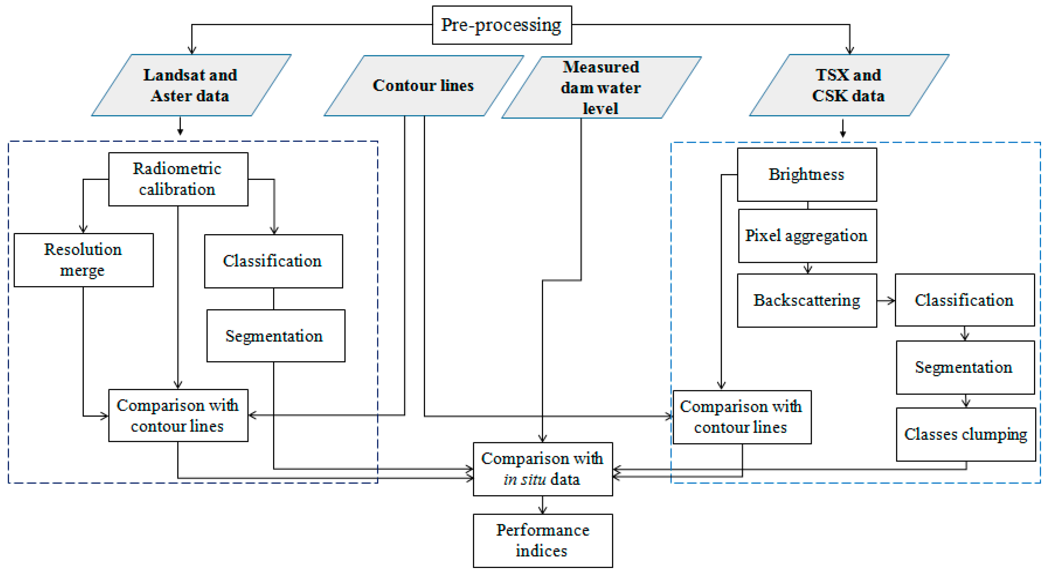
The unsupervised classification allowed estimation of the surface extension of the water body, while the subsequent segmentation enabled the exclusion of all pixels not connected with the water body but classified in the same class. The smallest segment was set equal to the number of pixels corresponding to a minimum reservoir surface during the entire time series (0.72 km², 12 September 2012); this minimum pixel number was varying with R_G. Connectivity was set equal to 4 neighbor pixels (

Table 5. Average reduction (± standard deviation) of inclusion and exclusion errors by applying segmentation and clumping on datasets with different geometric resolution.

	SAR		ASTER	LS8	LS5	LS7
RG	Stripmap 5.00	Scansar 8.25	15.00	30.00	30.00	30.00
Segmentation	−36.2 ± 16.9	−2.5	−2.9 ± 1.9	−1.1 ± 1.5	−0.5 ± 0.8	−0.2 ± 0.3
Clump	4.8 ± 4.8	0.8

).

The reduction, in terms of pixels classified as water surface is maximum for high-resolution grayscale images (~36 ± 17%, SAR Stripmap), and is small or even negligible for average resolution multispectral images (<3 ± 2%). Thus, image segmentation was particularly necessary over SAR images acquired at high geometric resolution. A class clumping algorithm was applied after segmentation by setting a 3 × 3 kernel. The clump allowed for the filling of pixels not classified as lake but positioned within the water body boundary. Water body boundary, conversely, was slight smoothed.

Segmentation statistic for ASTER images refer to three scenes acquired on the 3 August 2012 and 26 August 2012, and on the 9 May 2013. The other three images are characterized by partially cloudy conditions; for those images the average pixels’ reduction and standard deviation were ≈33.1 ± 1.9%. When clouds or shadows are positioned within the area of interest but do not cover the lake extension (e.g., ASTER scene acquired on the 1 January 2013, not shown here) segmentation produces a distinct segment that can therefore be removed. When clouds or shadows cover the lake extension (e.g., ASTER scene acquired on the 9 September 2011, not shown here), segmentation generates a unique segment causing an overestimation of the lake’s surface.

The clumping process was particularly effective over two CSK images acquired when the water surface was rough due to wind intensity and direction; over these images, a sharp increase in the number of pixels finally associated with the water body (~10%) was found.

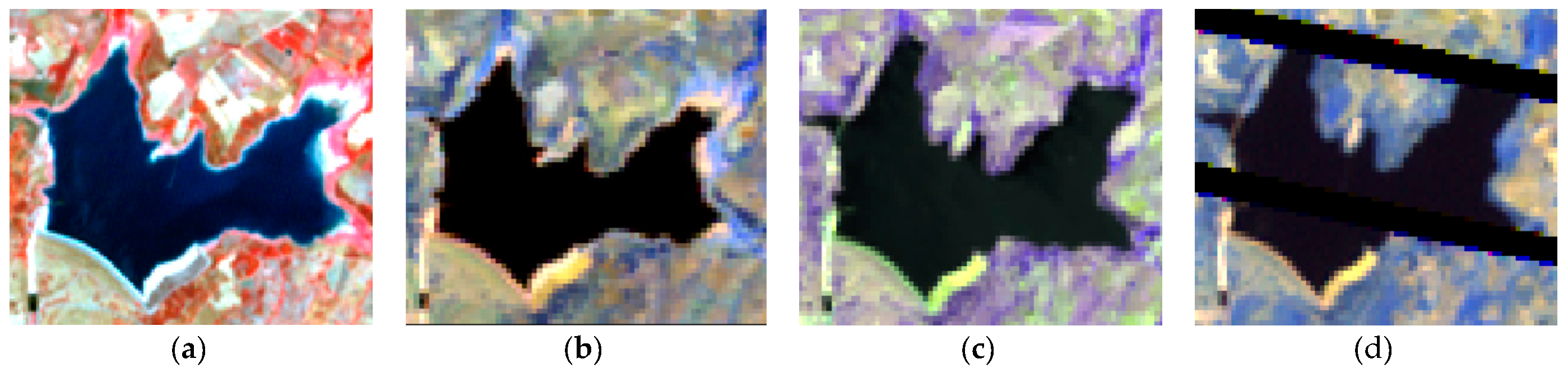
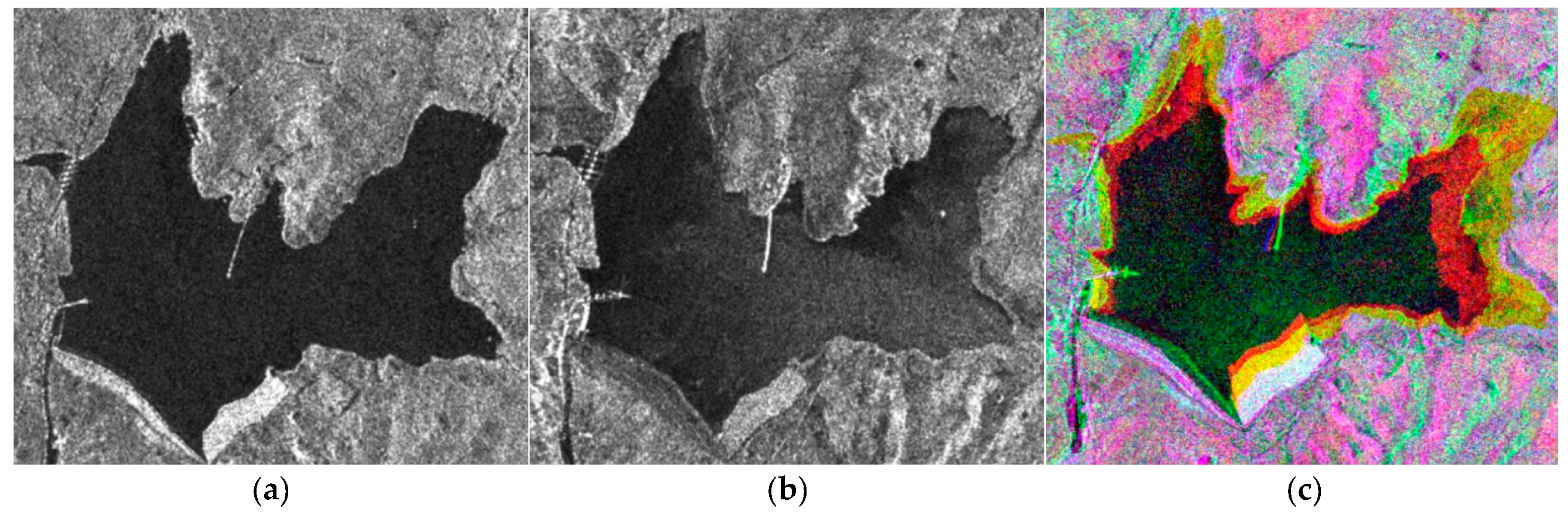
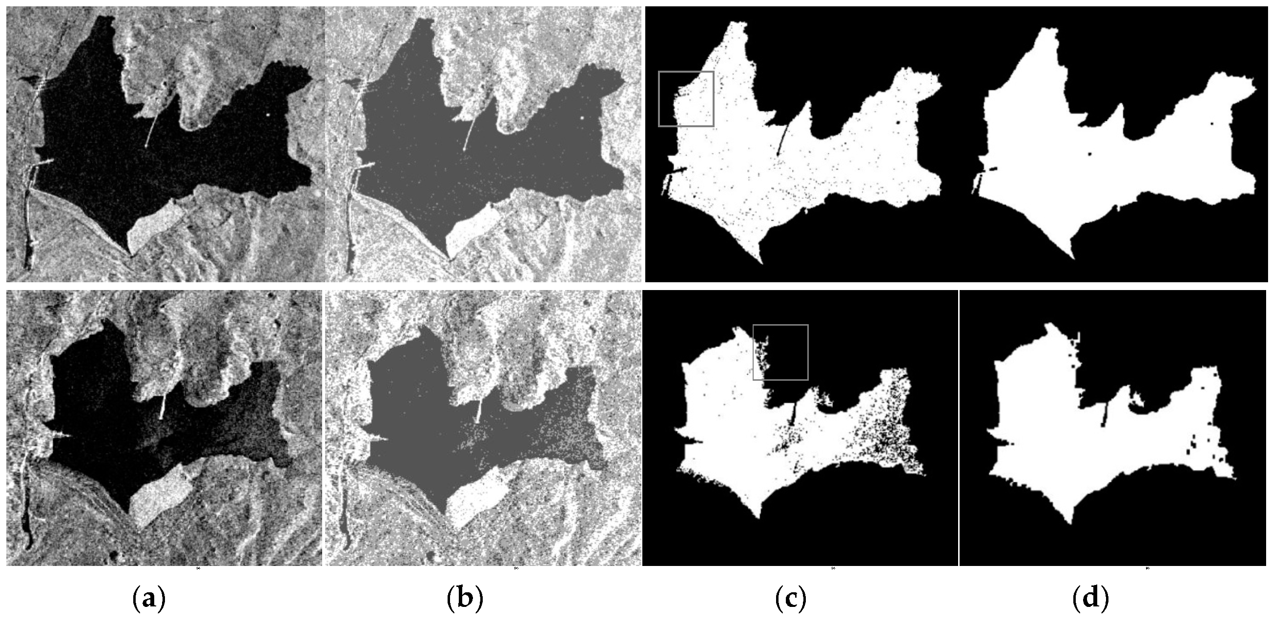
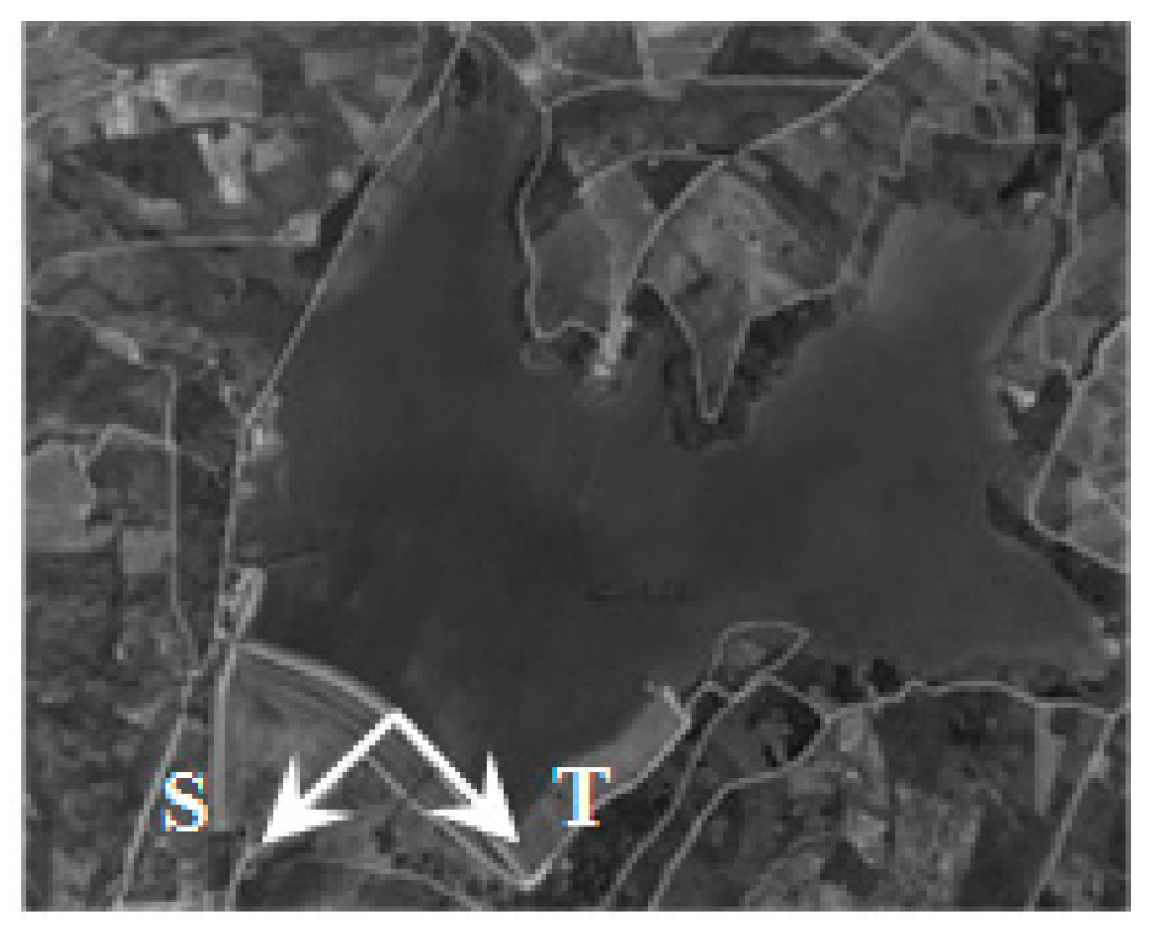
The classification of a CSK image acquired during a still day (Figure 8, upper panels) shows a clear delimitation of the main water body. Segmentation removed a small-disjoined segment since a branch of the reservoir was apparently disconnected from the main water body due to a bridge crossing it (west north-west zone of the reservoir, Figure 8c). A CSK image characterized by local windy conditions (10 September 2012) has shown limits in the classification performance (lower panels, a–d). Segmentation removes most of the pixels outside the water body even though some misclassified pixels remain (northern branch of the reservoir, lower panel, Figure 8c). The clumping process is not able to remove all pixels within the reservoir not classified as water (Figure 8d).

Although wind intensity and direction reduces the performance of the classification procedure, new radar satellites, such as the four radar satellites of the COSMO-SkyMed constellation offer a low revisit time (≤12 h for CSK) [36] comparable to in situ measurements (daily). Thus, discarding some images should not affect the operational applicability of the technique.

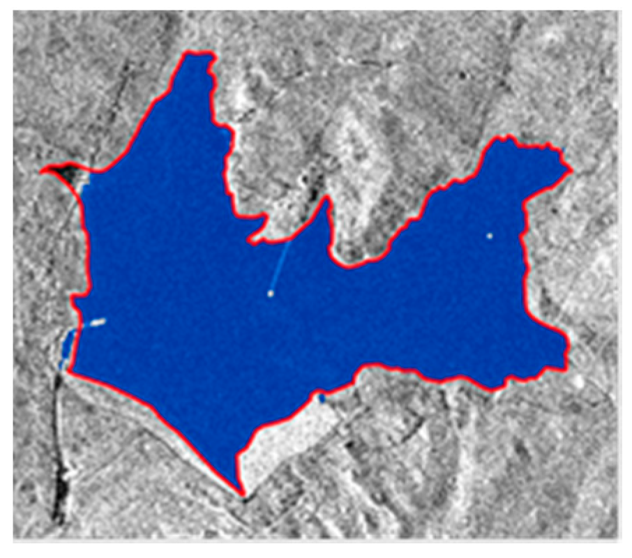
The comparison between the area resulting from the classification procedure (1.259 km², Figure 9, blue polygon) and the area evaluated via hand-digitization (1.265 km², red boundary) confirms the accuracy of the procedure (0.48% of underestimation for the selected still day CSK image).

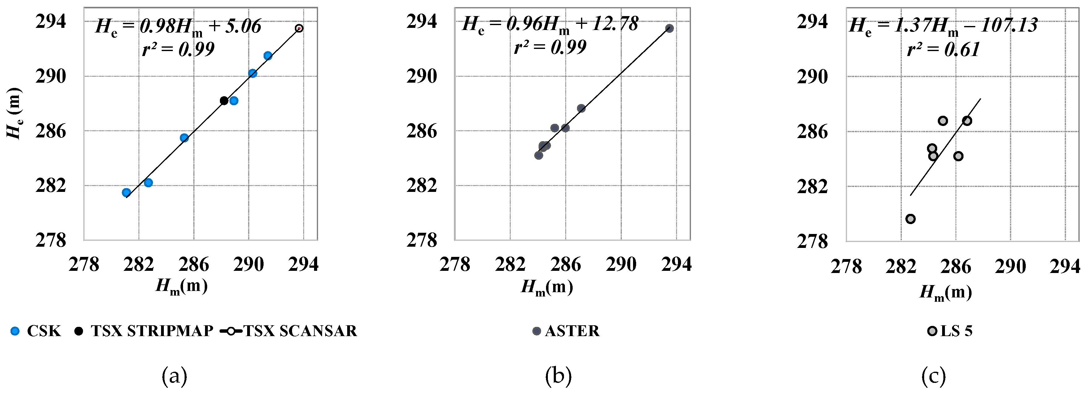
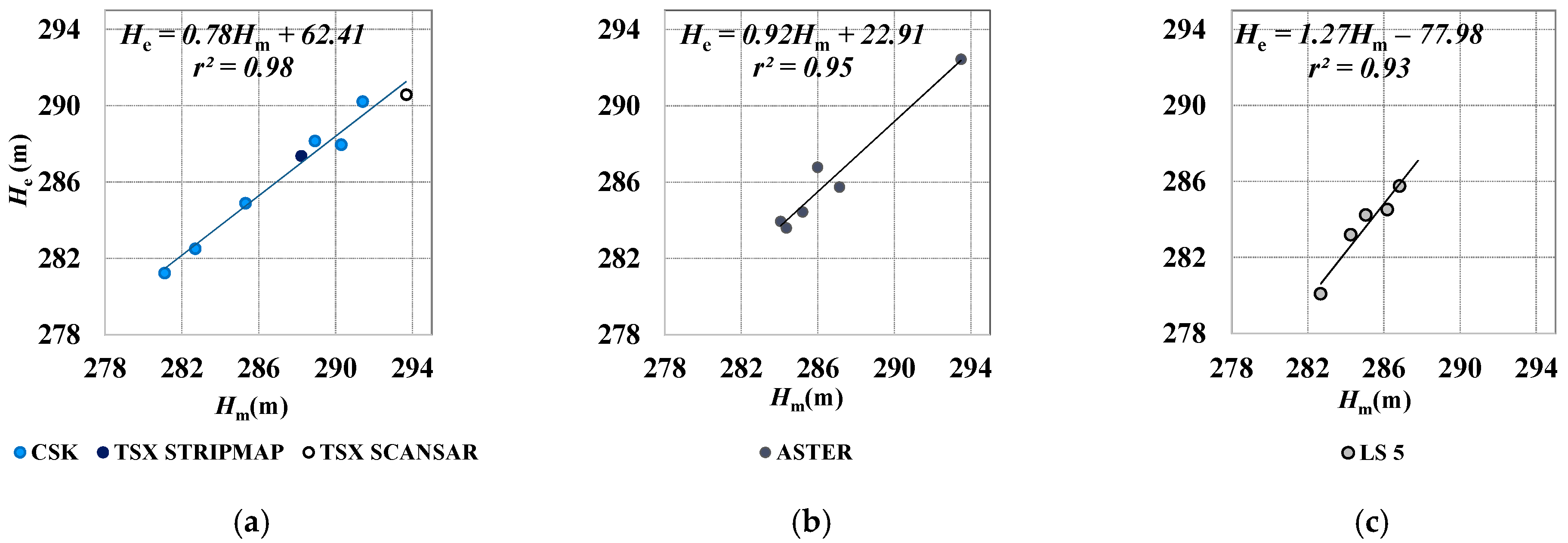
Water levels resulting from SAR, ASTER and LS5 processing are compared to water levels measured in situ (Figure 10a–c, respectively).

Both residual speckle and local wind speed and direction could influence SAR backscattering [37], thus SAR images require a specific setting of both segmentation and class clumping algorithms as specified in the methods section. Because water, σ₀ is similar to that characterizing surrounding land, images influenced by wind generally provide estimated levels lower than the measured ones.

Two partially cloudy ASTER images were not used after the classification, since this algorithm was not able to identify the water surface. Also, two LS5 images were not suitable for classification since the gap size did not allow an accurate water surface estimation. However, the estimated correlation was very high for all the different images (r² ~ 0.9). For LS5 data, the classification was applied just after a layer stacking representing the SWIR and NIR bands, because using all the MS available bands in many cases caused the classification process to fail, while using just the three bands meant the reservoir surface was easily determined.

Difficulties arise when RM was applied to LS8 and LS7 images. Despite an increase in the spatial resolution, the technique carries in the SWIR bands disturbances occurring in the visible bands. The panchromatic covers green, G, to NIR (specifically, 0.52 to 0.90 μm in LS7 and 0.50 to 0.68 μm in LS8). If applied on the whole MS images, RM damages SWIR bands when glint occurs in the visible bands. In these cases, water pixels are misclassified.

For that just the MS bands in the SWIR and NIR were used, with a resolution of 30 m, and then the segmentation process was applied. Before the classification, for LS7 SLC-Off data, the ENVI-IDL RBV method was used to fill the missing pixels inside the reservoir.

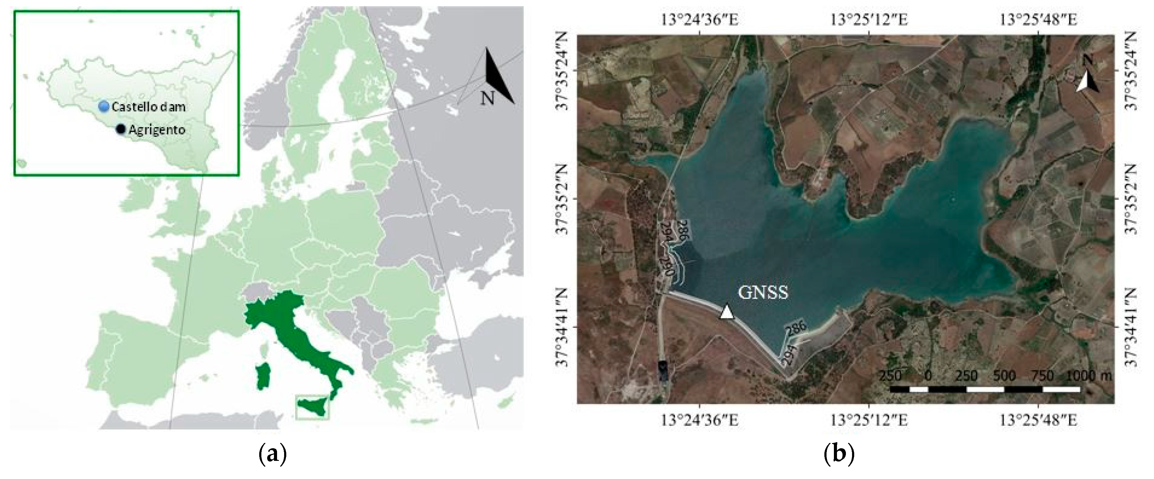
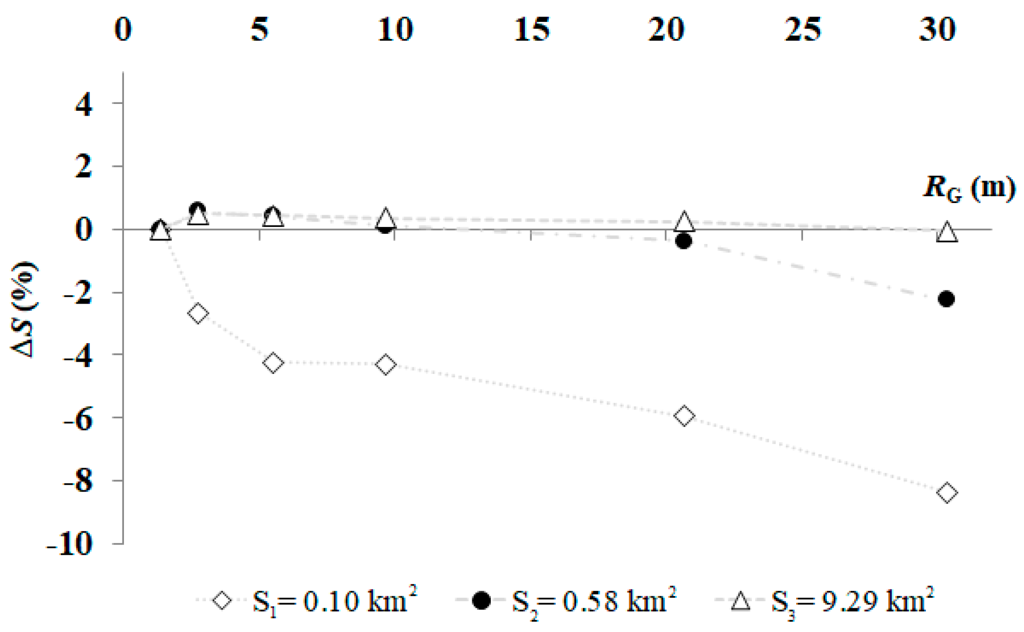
The reservoir is positioned on the central part of the Landsat scene 189/34 (~57 km from the left boundary) and on the lower right part of the Landsat scene 190/34 (~8 km from the right boundary). The position and the percentage of un-scanned rows and cloudiness inside the basin also differed. The average width of un-scanned rows is approximately 200 m for the scene 189/34, 400 m for the 190/34. In a previous work, the surface underestimation of a reservoir using the K-means clustering algorithm was analyzed, by applying synthetic stripes simulating the un-scanned rows in the LS7 SLC-Off data [16]. It was found that with the increasing ratio between total width of un-scanned rows (L_S) and length of the water body orthogonal to the scan line direction (L_L), came decreasing algorithm performance. Evaluated values of the characteristic ratios L_S/L_L were 0.033, 0.067, 0.133, and 0.200. A maximum underestimation of ~10% was considered suitable and using the MS bands, the obtained acceptable estimate for the ratio was lower than ~0.17.

Gaps characterizing the Castello dam on Magazzolo reservoir within the scene 189/34 have a characteristic ratio L_S/L_L < 0.17, thus the algorithm performance was considered satisfactory. On the contrary, L_S/ L_L over the scene 190/34 was higher than 0.2, thus these images were excluded from the analysis.

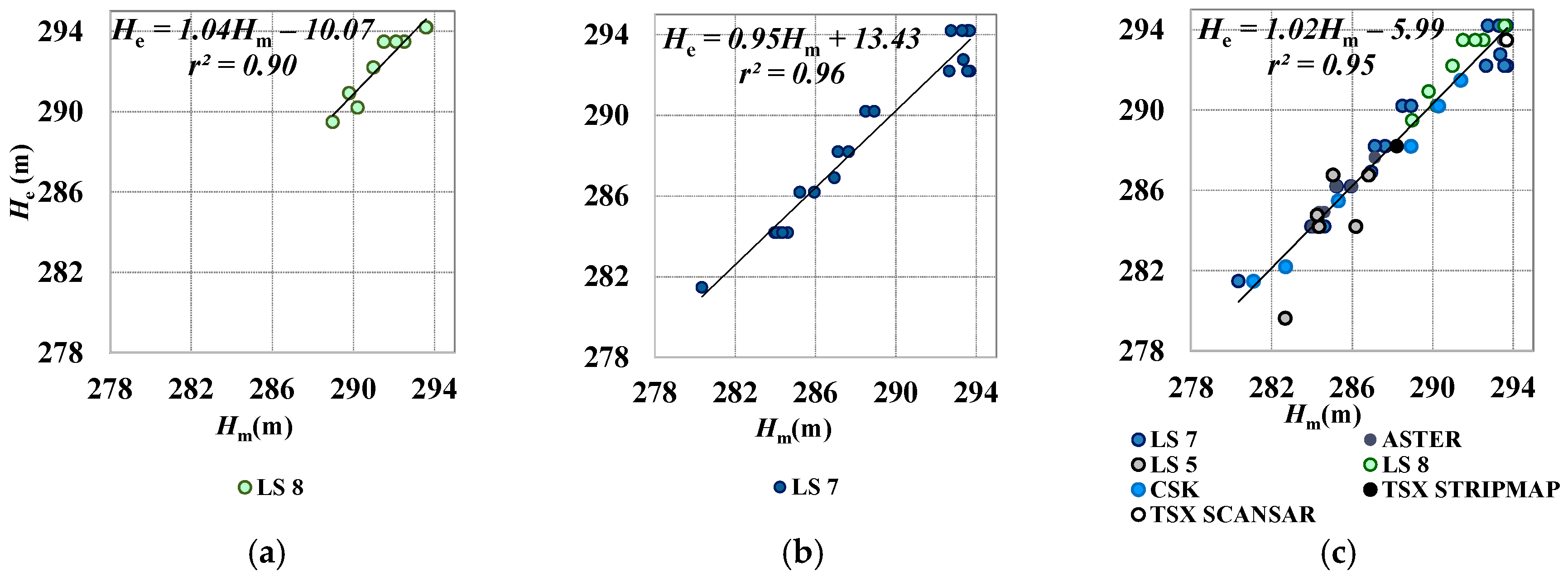
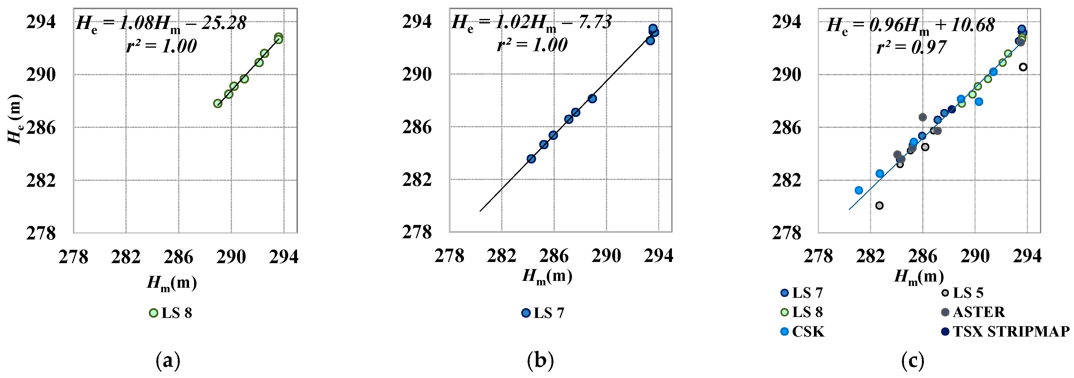
Moreover, some cases could occur where un-scanned rows are positioned along the dam or along a reservoir boundary that is almost parallel to the scan line. In both cases, because the loss of shape information, the RBV algorithm fails to rebuild the reservoir shape. Thus, all LS7 190/34 scenes (14 images) were excluded from the analysis, as well as two 189/34 scenes characterized by high clouds coverage or by missing scan lines coincident with the lake shoreline. Water levels estimated from LS8 and LS7 were compared to measured values (Figure 11).

Very high correlation (r² = 1.00) and low S.E. (0.14 and 0.21 m) were found between H_m and H_e derived from LS8 and LS7, respectively, although, few Landsat images were used (8 LS8 and 10 LS7). High correlation (r² > 0.9) was also found applying the classification method on the whole dataset, although S.E. was relatively high (0.70 m).

Although the unsupervised classification promises high performances, it presents many limitations. The method is influenced by cloudiness and shadows. When LS7 SLC-Off images need to be processed, the preliminary gap filling is a point of weakness for the accuracy of the subsequent classification. It needs to be highlighted that the position and the average width of the gap within the scene, for a given location, change with the acquisition path. In particular, it depends on the distance with the limits of the scene.

After the first screening of the dataset (cloud cover, scan-lines missing, shadows), 37 images were used for the analysis. Main statistical indicators used to evaluate the performance of the different methods are summarized in

Table 6. Main statistical indicators evaluating the performance of visual matching (M) and classification (C) techniques on different datasets. Best and worst values in black bold and blue bold, respectively.

	SAR		ASTER		LS8		LS5		LS7		All Data
	M	C	M	C	M	C	M	C	M	C	M	C
	(8)	(8)	(8)	(6)	(9)	(8)	(6)	(5)	(21)	(10)	(52)	(37)
m (−)	0.98	0.78	0. 96	0.92	1.04	1.08	1.37	1.27	0.95	1.02	1.02	0.96
q (m)	5.06	62.41	12.78	22.91	−10.07	−25.28	−107.13	−77.98	13.43	−7.73	−5.99	10.68
r (−)	1.00	0.99	1.00	0.98	0.95	1.00	0.78	0.96	0.98	1.00	0.98	0.98
S.E.(m)	0.38	0.58	0.30	0.81	0.61	0.14	1.83	0.65	0.86	0.21	0.92	0.70

. Statistics includes the slope (m), the intercept (q), r, S.E. and p value, for visual matching (M) and unsupervised classification (C) techniques, with the available number of images reported between parentheses. Best values are formatted in black bold, worst values in blue bold.

Main statistical indicators have shown that: (i) the classification procedure performed better on optical data when SWIR and NIR bands were used for visualization (LS7, m = 1.02, r = 1.00 and LS8, S.E. = 0.14 m, r = 1.00) while performed worst on optical images characterized by few spectral bands (this LS5 dataset, m = 1.27). Residual speckle and local wind effects on SAR single polarization (X_HH) band caused an underestimation of the water class (m = 0.78) although the correlation remained strong (r = 0.99); (ii) the visual matching produced best results on LS8 with a slight overestimate of the water levels (m = 1.04) although the correlation remained high (r = 0.95). Worst results occur when the technique is applied on LS5 images, with a strong overestimation (m = 1.37), low correlation (r = 0.78) and high standard error of the estimates (S.E. = 1.83 m). Also, for most of the analyzed dataset the correlation is significant and very strong (r > 0.9 and p < 0.01), just for LS5 with classification technique the p value highlights a lower significance (r = 0.78 and p = 6.7 × 10⁻²). Overall, the classification technique allows reaching a lower S.E. (0.70 m) and a significance level of 4.3 × 10⁻²⁷, although a limited number of images is suitable to be processed (<70% of the whole dataset in this case), while, the visual matching technique despite a higher S.E. (0.92 m) can be applied to almost the whole dataset (~90%) allowing a better estimate of the water level compared to the classification technique.

5.2. GNSS

After acquiring all the data from both the reference permanent station and the receiver positioned on the central part of the dam, the parameters for post-processing were set. RMS errors of processed baselines range between 0.54–1.17, 0.20–2.40 and 0.42–0.96 mm (X, Y and Z components, respectively). Average percentage of resolved ambiguities was 94.51%. Resulting coordinates were converted from geocentric to a local reference system (Figure 12), to obtain a displacement time series. Only horizontal components were analyzed since they were characterized by accuracy suitable to monitor the dam displacements. The horizontal accuracy after post-processing (≈1−5 × 10⁻³ m) was better than vertical (≈10−20 × 10⁻³ m), indeed the displacements time series has a more scattered behavior for the vertical component and the precision is one order of magnitude less than other traditional geodetic techniques (e.g., spirit leveling). A time averaging allowed the displacement behavior to emerge, although is characterized by a marked scattering.

Within this study, the displacements orthogonal to the dam for the central section were analyzed. Indeed, considering as first approximation the hydrostatic pressure acting orthogonally to the wall, the evaluation of any relation between the variables in the same direction seems to be interesting for a preliminary understanding of the deformation process. The actual deformation process of the earth dam appears too complex to be easily interpreted, since analogous displacements could be due to the different loads and rearrangements of the dam filling material during the emptying and filling periods.

The orthogonal displacements were monitored over two years, but several values are missing because of no-data acquisition or post-processing failures. However, a time series without gaps covers a cycle of emptying and filling phases (for an overall period of ~1 year).

The moving average (MA) was tested using different averaging periods (7, 14, 28 and 56 days). The results showed that the most reliable averaging period to evaluate the displacements of the dam through the receiver is about two months. Although, it could hide signal with shorter periods we are not interested in (e.g., real time monitoring). Displacements trend appears when the ≈ two months filter is applied. The MA of the displacements along S-axis shows a variability range of ±2 mm (Figure 13).

The two vertical dashed lines delimit: on the left, a period when water is used for irrigation and no rainfall occurs (until the 17 September 2011); a three months period within which the water level was quite stable (no water use, no rainfall); and on the right, a period characterized by no water use and rainfall (from 17 December 2011). The absolute minimum of the water level (H_m = 283.70 m) occurred within the central period, on the 20 October 2011 (white dot). Within the central period d_s standard deviation ranged between 1.39 and 2.05 mm, with 1.89 mm on the 20th of October. These values were similar to those occurring in the first and third periods (1.65–2.44 and 1.32–2.17 mm, respectively).

Preliminarily, displacements evaluated over ≈ two months MA were compared to water levels measured in situ to check if any relationship occurs. By averaging over time measured displacements a different behavior emerges during the emptying phase from the minimum water level (April 2011–September 2011) and the filling phases from the minimum water level (October 2011–March 2012). The minimum water level occurred when GNSS measured the maximum displacement.

5.3. Comparison between Displacements and Water Levels

Displacements evaluated via GNSS, water level measured in situ and estimated through remote sensing were compared during the one-year no-gaps displacements monitoring period (April 2011–March 2012). The monitoring period ranges from the emptying to the filling phase of the reservoir. Water levels derived from visual matching were used to enlarge the dataset.

The time behavior (Figure 14, left panel) shows that, a maximum displacement occurs when the lake was at its minimum level (20 October 2011, blue circle). However, the water level, apparently, does not fully explain the dam displacement behavior.

Indeed, a maximum dam displacement occurs in the middle of July 2011 (black circle) when daily average air temperature and water surface temperature reached their maxima values (30.5 °C on the 15 and 26.2 °C on the 18, respectively); while, a minimum dam displacement occurs during the second decade of February 2012 (black circle) when air and water temperatures reached their minima values (2.5 °C on the 11 and 8.2 °C on the 16, respectively).

A polynomial regression (red continuous lines, right panel) emphasized the behavior over the time of pairs water levels—displacements, highlighting a difference between the emptying phase until minimum (upper curve, green dots) from filling phase from minimum (lower curve, blue dots). A hysteresis-like loop seems to describe the time behavior of the pairs during a whole hydrological cycle (April 2011–March 2012), probably due to the different rearrangements of the dam filling material and loads applied during the different periods.

6. Conclusions and Recommendations

The analyses highlight the advantages of using satellite technologies to determine dam displacements and reservoir water level.

Two methods for the determination of the water level were tested to point out benefits and disadvantages if applied on images with different radiometric and geometric contents (optical and SAR). The classification method failed over cloudy or shadowed images (~7% of the original dataset) while, over SLC-off images, its performance decays abruptly with un-scanned row width. The average width of un-scanned rows and the ratio L_S/L_L were calculated for both 189/34 and 190/34 scenes over the Castello dam on Magazzolo reservoir. L_S/L_L was less than 0.17 on 189/34 images, thus the performance of the gap filling algorithm was considered satisfactory; 190/34 images, on the contrary, have a ratio higher than 0.2, thus these images were excluded from the analysis.

Performances of the visual matching method reside in the operator ability to distinguish wet ground from shallow water. A false-color composition needs to be chosen to enhance this visual separability. Considering how the spectral behavior of the diffuse attenuation coefficient influences the emerging radiance, the spectral bands facilitating the discrimination between land and water were SWIR and NIR bands when available (LS images), or just VNIR bands otherwise (ASTER images). The visualization of SAR images (here single band and polarization) is limited to grey-scale.

The application of the resolution merge based on principal component analysis increased the spatial resolution of optical images, thus facilitating the delimitation of the water bounds within the visual matching technique. Radiometric distortions, however, could be introduced in visible bands even if glint occurs only on NIR bands, thus damaging images suitable to be classified with an unsupervised technique. This is due to the high spatial-low spectral resolution panchromatic image substitutes the first PC of the low spatial-high spectral resolution multispectral images, and then the inverse principal component transformation is applied to obtain the high spatial-high spectral RM images. Thus, features such as sun glint, visible in the PAN image since it covers also NIR in LS7 and LS8, should not be introduced in visible bands.

The speckle noise of SAR images decreases with increasing pixel aggregation, thus different levels of aggregation were tested. The optimum level of aggregation was identified in this study as the multiple R_G for which the difference between H_e and H_m was minimized. The spatial resolution characterizing the optimum level of aggregation was 5 m for Stripmap, R_G was left equal to 8.25 m for Scansar.

Moreover, backscattering depends on wind speed and direction influenced by local morphology. Indeed, analyzing hourly wind speed and direction recorded from a weather station (≈2 km North direction), when roughness of surfaces was remotely sensed the averaged wind speed was higher than 1.5 ms⁻¹ in the hours before the time acquisition and the wind direction (at 2 m height) was aligned with the look direction.

Segmentation and class clumping algorithms allow dealing with speckle, wind, clouds, and shadow influences on optical and SAR images. Segmentation allowed removing misclassified pixels outside the reservoir (inclusive errors). Despite SAR images being aggregated to minimize the speckle effects, several pixels within the reservoir are misclassified due to residual noise; indeed, residual speckle reduces the classification performances. Segmentation of SAR classified images reduces misclassified pixels up to ~36% on average (Stripmap images, R_G = 5 m). Segmentation of classified clear sky optical images reduces inclusive errors up to ~3% on average. Clumping allowed removing misclassified pixels within the reservoir (exclusive errors). It is required on SAR images. Clumping of classified Stripmap images reduces exclusive errors up to ~10%.

Clouds covering a reservoir limit the applicability of the classification method. The position and width of un-scanned rows, especially when these are positioned along the dam structure or on the upper bound of the lake, reduces the accuracy of the classification. Results showed a strong correlation between H_m and H_e (r² ranged between 0.93 using LS5 and 1.00 using LS8 and LS7, it reached 0.97 using the whole dataset) although a limited number of images were used (<70 % of the dataset).

Conversely, the visual matching relies on the geometric content and data planimetric positioning accuracy of the images; moreover, the method is influenced by the operator subjectivity. However, it allows employing a more robust dataset (90% of the whole dataset), even if the reservoir is partly covered by clouds of shadows or partly un-scanned (e.g., Landsat 7 SLC-Off images). The comparison between H_m and H_e using this method has shown a strong correlation as well, with r² ranging between 0.61 (LS5) and 0.99 (SAR and ASTER), and 0.95 using the whole dataset, just for LS5 images the p value highlights a lower significance (6.7 × 10⁻²).

GNSS allows evaluating displacements of the crest of the dam continuously over the time. Contrasting with other authors (e.g., [5]) the baseline employed a permanent station relatively far away from the study site (AGRI, ~30 km). The planimetric component of the displacements appears to be sensitive to sub-centimeter displacements. The use of a relatively distant permanent station reduced the materialization costs and allows excluding that the base station is influenced by the dam deformation or the reservoir emptying-filling cycle. Due to failures of data acquisition or post-processing, a continuous displacements time series is available for just ~1 year. Even though, the ≈two month moving average allowed the displacements trend to emerge.

Finally, the displacements evaluated from GNSS were compared with water levels measured in situ and derived from remote sensing visual matching, despite a limited number of images were acquired during the no-gap GNSS monitoring period. Displacements during emptying and filling phases of the reservoir show different response to water levels. Water level seemingly does not fully explain the dam displacement behavior; indeed, a secondary maximum displacement occurs when air and water temperatures reach their maxima, while a minimum occurs when temperatures reach their minima.

A different behavior during the emptying and filling phases (April 2011–March 2012) was found to form a hysteresis-kind loop. However, time averaged displacements are characterized by high standard deviation (±2 mm). Other authors found an apparent linear relationship between water levels and dam deformations (e.g., [6,16]), while others found a non-perfect correlation between radial displacements and water levels [7]; thus, different interpretations could emerge when a short time series is analyzed. Thus, further analyses are required to interpret the displacements response to the water level.

References

1. Szostak-Chrzanowski, A.; Massiéra, M. Modelling of deformations during construction of a large earth dam in The La Grande Complex, Canada. Tech. Sci. 2004, 7, 109–122. [Google Scholar]
2. Drummond, P. Combining Cors Networks, Automated Observations and Processing, for Network Rtk Integrity Analysis and Deformation Monitoring. In Proceedings of the 15th FIG Congress Facing the Challenges-Building the Capacity, Sydney, Australia, 11–16 April 2010. [Google Scholar]
3. Taşçcedil, L. Analysis of dam deformation measurements with the robust and non-robust methods. Sci. Res. Essays 2010, 5, 1770–1779. [Google Scholar]
4. Duffy, M.; Hill, C.; Whitaker, C.; Chrzanowski, A.; Lutes, J.; Bastin, G. An automated and integrated monitoring program for Diamond Valley Lake in California. In Proceedings of the 10th FIG International Symposium on Deformation Measurements, Orange, CA, USA, 19–22 March 2001. [Google Scholar]
5. Tarsisius Aris, S.; Kabul Basah, S.; Fakrurazzi, D.; Adin, S.; Adhi, D.; Susilo, A. Design and installation for Dam Monitoring Using Multi sensors: A Case Study at Sermo Dam, Yogyakarta Province, Indonesia. In Proceedings of the FIG Working Week 2012, Knowing to Manage the Territory, Protect the Environment, Evaluate the Cultural Heritage, Rome, Italy, 6–10 May 2012. [Google Scholar]
6. Bayrak, T. Verifying Pressure of Water on Dams, a Case Study. Sensors 2008, 8, 5376–5385. [Google Scholar] [CrossRef] [PubMed] [Green Version]
7. Kalkan, Y. Geodetic deformation monitoring of Ataturk Dam in Turkey. Arab. J. Geosci. 2014, 7, 397–405. [Google Scholar] [CrossRef]
8. Yigit, C.O.; Alcay, S.; Ceylan, A. Displacement response of a concrete arch dam to seasonal temperature fluctuations and reservoir level rise during the first filling period: evidence from geodetic data. Geomat. Nat. Hazards Risk 2016, 7, 1489–1505. [Google Scholar] [CrossRef]
9. Gao, H.; Birkett, C.; Lettenmaier, D.P. Global monitoring of large reservoir storage from satellite remote sensing. Water Resour. Res. 2012, 48, W09504. [Google Scholar] [CrossRef]
10. Kleine, I.; Rogass, C.; Medeiros, P.H.A.; Erpen, N.M.; Francke, T.; Bronstert, A.; Förster, S. Comparison of approaches for water surface area segmentation using high resolution TerraSAR-X data for reservoir monitoring in a large semi-arid catchment in north eastern Brazil. In Proceedings of the 2013 SPIE Remote Sensing, Dresden, Germany, 23–26 September 2013. [Google Scholar]
11. Sima, S.; Tajrishy, M. Using satellite data to extract volume-area-elevation relationships for Urmia Lake, Iran. J. Great Lakes Res. 2013, 39, 90–99. [Google Scholar] [CrossRef]
12. Crétaux, J.-F.; Bergé-Nguyen, M.; Calmant, S.; Romanovski, V.V.; Meyssignac, B.; Perosanz, F.; Tashbaeva, S.; Arsen, A.; Fund, F.; Martignago, N.; et al. Calibration of Envisat radar altimeter over Lake Issykkul. Adv. Space Res. 2013, 51, 1523–1541. [Google Scholar] [CrossRef]
13. Birkett, C.M.; Beckley, B. Investigating the performance of the Jason-2/OSTM Radar Altimeter over Lakes and Reservoirs. Mar. Geodesy 2010, 33, 204–238. [Google Scholar] [CrossRef]
14. Shimizu, N. Rock Displacement Monitoring using Satellite Technologies-GPS and InSAR. In Proceedings of the ISRM VietRock International Workshop, Hanoi, Vietnam, 12–13 March 2015. [Google Scholar]
15. Lazecky, M.; Perissin, D.; Lei, L.; Qin, Y.; Scaioni, M. Plover Cove Dam Monitoring with Spaceborne InSAR Technique in Hong Kong. In Proceedings of the 2nd Joint International Symposium on Deformation Monitoring (JISDM), Nottingham, UK, 9–10 September 2003. [Google Scholar]
16. Dardanelli, G.; La Loggia, G.; Perfetti, N.; Capodici, F.; Puccio, L.; Maltese, A. Monitoring displacements of an earthen dam using GNSS and remote sensing. In Proceedings of the 2014 SPIE Remote Sensing, Amsterdam, The Netherlands, 22–25 September 2014. [Google Scholar]
17. Dardanelli, G.; Pipitone, C. Hydraulic models and finite elements for monitoring of an earth dam, by using GNSS techniques. Period. Polytech. Civ. Eng. 2017, 61, 421–433. [Google Scholar] [CrossRef]
18. Thome, K.; Markham, B.; Barker, J.; Slater, P.; Biggar, S. Radiometric calibration of Landsat. Photogramm. Eng. Remote Sens. 1997, 63, 853–858. [Google Scholar]
19. Epema, G.F. Effect of moisture content on spectral reflectance in a playa area in Southern Tunisia. In Proceedings of the International Symposium Remote Sensing and Water Resources, Enschede, The Netherlands, 20–24 August 1990; pp. 301–308. [Google Scholar]
20. Airbus Defence & Space. Radiometric Calibration of TerraSAR-X Data-Beta Naught and Sigma Naught Coefficient Calculation. Document: TSXX-ITD-TN-0049-radiometric_calculations_I3.00.doc. March 2014. Available online: https://spacedata.copernicus.eu/documents/12833/14537/TerraSAR-X_RadiometricCalculations (accessed on 5 January 2018).
21. E-Geos. COSMO SkyMed Image Calibration. Document: COSMO-SkyMed-Image_Calibration.pdf. Available online: http://www.e-geos.it/products/pdf/COSMO-SkyMed-Image_Calibration.pdf (accessed on 3 January 2017).
22. Ciraolo, G.; Cox, E.; La Loggia, G.; Maltese, A. The classification of submerged vegetation using hyperspectral MIVIS data. Ann. Geophys. 2006, 49, 287–294. [Google Scholar]
23. Welch, R.; Ehlers, W. Merging Multiresolution SPOT HRV and Landsat TM Data. Photogramm. Eng. Remote Sens. 1987, 53, 301–303. [Google Scholar]
24. Tou, J.T.; Gonzalez, R.C. Pattern Recognition Principles; Addison-Wesley Publishing Company: Reading, MA, USA, 1974; pp. 97–104. [Google Scholar]
25. Jensen, J.R. Introductory Digital Image Processing; Prentice-Hall: Englewood Cliffs, NJ, USA, 1986; p. 379. [Google Scholar]
26. Liebe, J.R.; van de Giesen, N.; Andreini, M.S.; Steenhuis, T.S.; Walter, M.T. Suitability and Limitations of ENVISAT ASAR for Monitoring Small Reservoirs in a Semiarid Area. IEEE Trans. Geosci. Remote Sens. 2009, 47, 1536–1547. [Google Scholar] [CrossRef]
27. Saastamoinen, J. Atmospheric correction for troposphere and stratosphere in radio ranging of satellites. In The Use of Artificial Satellites for Geodesy; Henriksen, S.W., Mancini, A., Chovitz, B.H., Eds.; AGU: Washington, WA, USA, 1972; Volume 15, pp. 247–252. [Google Scholar]
28. Niell, A.E. Global mapping functions for the atmosphere delay at radio wavelengths. J. Geophys. Res. 1996, 101, 3227–3246. [Google Scholar] [CrossRef]
29. Klobuchar, J.A. Ionospheric Effects on GPS. In Global Positioning System: Theory and Applications; American Institute of Aeronautics and Astronauitc: Reston, VA, USA, 1996; Chapter 12; Volume 1, pp. 485–515. [Google Scholar]
30. Schwiderski, E.W. On charting global ocean tides. Rev. Geophys. Space Physics. 1980, 18, 243–268. [Google Scholar] [CrossRef]
31. De Martino, P.; Tammaro, U.; Obrizzo, F.; Sepe, V.; Brandi, G.; D’Alessandro, A.; Pingue, M.D.E.F. The GPS network of Ischia Island: Ground deformations in an active volcanic area (1998–2010). Quad. Geofis. 2011, 95, 95. [Google Scholar] [CrossRef]
32. Panza, G.F.; Peresan, A.; Magrin, A.; Vaccari, F.; Sabadini, R.; Crippa, B.; Marotta, A.M.; Splendore, R.; Barzaghi, R.; Borghi, A.; et al. The SISMA prototype system: Integrating Geophysical Modeling and Earth Observation for time-dependent seismic hazard assessment. Nat. Hazards 2013, 69, 1179–1198. [Google Scholar] [CrossRef]
33. Fermi, M.; Caldera, S.; Chersich, M.; Osmo, M. Validazione del software NDA Professional per la compensazione di reti di stazioni permanenti GNSS. In Proceedings of the 14a Conferenza Nazionale ASITA, Brescia, Italy, 9–12 November 2010. [Google Scholar]
34. Dardanelli, G.; Sciortino, M. Time series analysis in the UNIPA NRTK GNSS network. In Proceedings of the 5th International Conference and Exhibition, Melaha, Location Technologies and Solutions: The Next Frontier, Cairo, Egypt, 3–5 May 2010. [Google Scholar]
35. Dardanelli, G.; Franco, V.; Lo Brutto, M. La rete GNSS per il posizionamento in tempo reale dell’Università di Palermo: progetto, realizzazione e primi risultati. Boll. SIFET 2008, 2, 107–124. [Google Scholar]
36. Italian Space Agency. COSMO-SkyMed. Document: ASI-CSM-PMG-NT-001 COSMO-SkyMed Mission and Products Description.pdf. Available online: http://www.e-geos.it/images/documents/COSMO-SkyMed%20Mission%20and%20Products%20Description.pdf (accessed on 3 January 2017).
37. Clemente-Colón, P.; Yan, X.H. Low-Backscatter Ocean Features in Synthetic Aperture Radar Imagery. Johns Hopkins APL Tech. Dig. 2000, 21, 116–121. [Google Scholar]
Figure 1. Flow diagram of optical and SAR imagery processing.
Remotesensing 10 00071 g001
Figure 2. (a) Geographical position of the study area; (b) satellite view of the Castello dam with over imposed the GNSS reference station position.
Remotesensing 10 00071 g002
Figure 3. (a) A pseudo-color composition (VNIR bands) of an ASTER image (3 August 2012, 15 m); (bd) pseudo-color compositions (SWIR1, 2 and NIR bands) of LS5 (28 August 2011, 30 m), LS8 (11 June 2013, 30 m) and LS7 (13 May 2011, 30 m) images, respectively.
Remotesensing 10 00071 g003
Figure 4. Smooth and rough water surfaces (left and central panels, respectively) sensed by CSK on the 23 June and 15 February 2012, and diachronic CSK false-color composition for increasing Hm, (281.10, 285.31 and 291.40 m represented in red, gran and blue color scales, respectively).
Remotesensing 10 00071 g004
Figure 5. ΔS at varying RG over different lake sizes.
Remotesensing 10 00071 g005
Figure 6. Water level measured in situ (Hm) versus levels obtained by visual matching technique (He) using: (a) SAR; (b) ASTER and (c) LS5.
Remotesensing 10 00071 g006
Figure 7. Water levels measured in situ (Hm) vs. levels obtained by visual matching (He) using: (a) LS8; (b) LS7; (c) all data.
Remotesensing 10 00071 g007
Figure 8. CSK acquired on the 08th of February 2012 during still day (upper panels) and on the 10 September 2012 during windy conditions (lower panels). (a) Backscattering σ0; (b) unsupervised classification; (c) segmented image; (d) clumped image.
Remotesensing 10 00071 g008
Figure 9. CSK acquired on the 8 February 2012, over-imposed a polygon extracted from the classification procedure (in blue) and a hand-digitized water surface (red boundary).
Remotesensing 10 00071 g009
Figure 10. Water levels measured in situ (Hm) vs. levels evaluated through classification (He) using: (a) SAR; (b) ASTER; (c) LS5 data. The water level was derived from the specific surface-level relationship of the reservoir.
Remotesensing 10 00071 g010
Figure 11. Water levels measured in situ (Hm) vs. levels evaluated trough classification (He) using: (a) LS8; (b) LS7; (c) all data.
Remotesensing 10 00071 g011
Figure 12. Local reference system (T and S indicate directions tangential and orthogonal to the dam).
Remotesensing 10 00071 g012
Figure 13. Temporal behavior of timely averaged GNSS displacements of the central section along S-axis (black dots) with over imposed ± the standard deviation within the 2 months moving window (yellow bars). Vertical dashed lines delimit a period of water use and no rainfall (on the left), a period of no water use and no rainfall (central); a period of no water use and rainfall (on the right). The white dot indicates ds occurring with minimum the water level.
Remotesensing 10 00071 g013
Figure 14. On the left panel: Time behavior of the water level from measurements in situ (Hm, black line) and visual matching (He, big circles) during the emptying phase until the minimum (in green) and filling phase (in blue) from the minimum (primary y-axis,) and GNSS time averaged displacements (dS) (green and blue lines, secondary y-axis). On the right panel, He, and Hm, vs. dS. during the emptying (green circles) and filling (blue circles) phase, over-imposed two interpolation curves (red continuous lines).
Remotesensing 10 00071 g014