1. Introduction
Satellite remote sensing techniques are very useful and powerful tools that have helped us to acquire in-depth knowledge of the Earth’s surface environment and its interior over the past few decades. These techniques play important roles in research fields including hydrology, ecology, oceanography, glaciology and geology. Among the current spaceborne techniques, global navigation satellite system reflectometry (GNSS-R) is an effective and innovative remote sensing technique for the ocean, land and cryosphere [
1,
2]. It can be used to derive geophysical parameters based on the GNSS L-band signals that are reflected by the Earth’s surface under all weather conditions [
3,
4,
5,
6,
7].
Accurate sea surface heights and wind direction/speeds have been retrieved based on GNSS-R observations from different ground-based, airborne and spaceborne platforms [
8,
9,
10,
11,
12]. The sea/ice transition was observed using GNSS-R bi-static radar images generated from TechDemoSat-1 (TDS-1) Delay Doppler Maps (DDMs) [
13]. Phase altimetry over sea ice was performed using high-precision Global Positioning System (GPS) carrier phase measurements extracted from TDS-1 coherent GNSS reflections [
14]. The surface’s reflectivity and variability of snow and ice surfaces interacting with GPS L1 and L2 signals were investigated using the direct and reflected polarizations of each signal [
15]. An overview of the challenges and status of the determination of soil moisture and snow properties in alpine environments was provided by Botteron et al. [
16]. The accuracy of GPS interferometric reflectometry for soil moisture and snow depth was evaluated by Larson [
17]. An algorithm of sea target detection from spaceborne GNSS-R DDMs was tested and validated using TDS-1 GNSS-R data [
18]. Besides, GNSS-R experiments for various land remote sensing applications, such as soil moisture, agriculture and forest elements, have been successfully tested [
7,
19,
20]. Thus, it can be seen that previous experimental and theoretical works show that GNSS-R are very useful. In addition, some studies for simulated scenario had been performed. Valencia et al. [
21] performed a comprehensive simulation to assess the impact of the observation geometry on the GNSS-R observable directly used to describe ocean surface’s roughness. An effective technique to reconstruct the normalized radar cross-section image from GNSS-R DDM had been applied to simulated noise DDMs [
22]. However, this method provides a wide swath and improved spatiotemporal sampling when compared with other spaceborne missions. Since a few spaceborne GNSS-R missions have been realized to date and several GNSS systems are under construction at present, there is a lack of datasets obtained from real space-based measurements covering dual-band signals from multiple constellations (e.g., GPS, Global Navigation Satellite System (GLONASS), the Galileo satellite navigation system (Galileo), and the BeiDou Navigation Satellite System (BDS)). In this paper, we perform simulations and analyses to evaluate the characteristics of ground-based reflected signals in terms of longitudinal/latitudinal variability and revisit time in the presence of future multiple constellations of GNSS satellites with nearly 120. The spaceborne GNSS-R payload generally consists of one or two nadir-oriented left-hand circularly polarized (LHCP) antenna, a zenith-oriented right-hand circularly polarized (RHCP) antenna, and a specialized GNSS-R receiver [
23,
24,
25]. Because the payload does not contain a transmitter and is small enough to be installed on a micro-satellite, GNSS-R is a low-cost passive remote sensing space technique with low power consumption. Consequently, it is possible to launch several LEO (low Earth orbit) micro-satellites into orbit at altitudes of approximately 500 km using a single rocket to form a GNSS-R constellation. In addition, as increasing numbers of available GNSS satellites will transmit L-band navigation signals in the future, this technique offers the advantage of enabling Earth surface observation with unprecedentedly high temporal resolution when compared with other traditional satellite missions.
We can now forecast that the future state-of-the-art GNSS-R Earth observation system will consist of several LEO observatories and approximately 120 GNSS satellites from multiple constellations. Unlike active space-based remote sensing techniques, the observation areas of the GNSS-R system are centered on specular reflection points on the Earth’s surface between the GNSS transmitters and the LEO receivers rather than on the nadir points. Many researchers worldwide have studied GNSS-R through various simulations and analyses. In 1998, several criteria for altimetry using reflected GPS signals were addressed, including the required signal strength, the required delay characteristics and an algorithm for computation of the specular reflection position between the GPS and the LEO receiver [
26]. In 2003, the TOPEX/Poseidon and Challenging Minisatellite Payload (CHAMP) satellites were used as GPS-R observatories and the distributions of ocean reflections from GPS satellites were simulated [
27]. Klokočník et al. [
28] proposed that a resonance orbit could be used to enhance the ground track density of GNSS-R LEO satellites. In 2006, Germain and Ruffini [
29] presented the performances of two proposed GNSS-R altimetry space missions. The results showed that the required antenna gain in the case of 700-km orbit height was higher than that in the case of 500-km orbit height [
29]. In 2017, Camps et al., analyzed the altimetric root mean square error of ESA (European Space Agency) proposed GEROS-ISS (GNSS Reflectometry, Radio Occultation and Scatterometry-International Space Station) mission for the minimum (330 km) and maximum (460 km) ISS orbital heights [
30]. In recent years, some researchers have begun to consider the spatial and temporal resolutions of GNSS-R anew because of the NASA (National Aeronautics and Space Administration) mission called the Cyclone Global Navigation Satellite System (CYGNSS). At the end of 2016, NASA launched the CYGNSS mission, which used eight micro-satellites; each individual observatory can track up to four parallel reflected GPS L1 signals [
24]. The medium and mean revisit times for CYGNSS missions were computed using an empirical distribution. The results showed that the median time is 2.8 h and the mean revisit time is 7.2 h when calculated across the entire 13-day cycle. Zavorotny et al. [
31] showed that the mean revisit time over the equatorial regions with an approximate latitude range of ±38° is approximately 5 h, but they may have adopted a different strategy from that of Ruf et al. [
24]. In addition, Zavorotny et al. [
31] performed a coverage and revisit time simulation for a possible GNSS-R constellation consisting of 24 polar orbiting satellites, with each of these satellites tracking up to 10 parallel reflections from both GPS and Galileo satellites. The average revisit time for this system was less than 2 h globally. However, researchers have seldom studied the potential performance of GNSS-R when four GNSS systems are fully operational and detailed simulation methods and results have not been published to date.
The precursor of CYGNSS is TDS-1 mission launched in July 2014, which carried a GNSS-R payload called the Space GNSS Receiver Remote Sensing Instrument (SGR-ReSI). An updated revision of the SGR-ReSI was selected as payload on each satellite of CYGNSS mission. This instrument on TDS-1 could receive GPS L1 and L2C signals and gathered many useful and important spaceborne GNSS-R data for scientific research [
32]. Much of the data from TechDemoSat-1 GNSS-R experiment has been made available at the MERRByS website and analyzed to perform geophysical parameter retrievals [
14,
15,
18].
On August 15th, 2016, a Spanish experimental GNSS-R
3cat-2 satellite with a PYCARO (P (Y) and C/A reflectometer) payload that can receive reflected signals from different GNSS satellites was launched using the CZ-2D (2) rocket at China’s Jiuquan Space Center [
25]. This mission proves that the four-system GNSS-R system will be feasible in future. Additionally, other GNSS-R missions such as the PARIS-IoD (Passive Reflectometry and Interferometry System In-orbit Demonstration) and GEROS missions are also in progress [
33,
34].
Increasing numbers of GNSS satellites will be operational in the next few years. Galileo will reach full operational capability (FOC) in 2020 [
35]. China is also in the process of expanding its regional BDS to form the global BeiDou-3 GNSS by 2020 [
36]. Approximately 120 GNSS satellites in orbit, including GPS, GLONASS, Galileo and BDS satellites, will be available for use as illuminators in a few years. The upcoming GNSS-R constellations should therefore receive more and better reflected signals simultaneously from all four main GNSS constellations. If this concept can be realized, then the coverage and revisit times of GNSS-R constellations will be upgraded to higher levels.
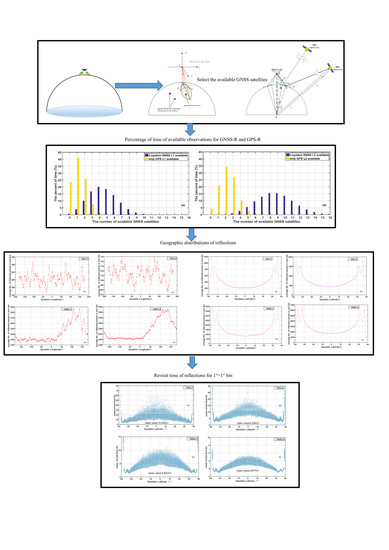
To meet the specific requirements of a variety of missions, including monitoring of the sea surface height and surface winds, and detection of sea surface ice and other large targets, it is important to quantize the observation capacity exactly during the mission design phase. Analysis and evaluation processes are thus necessary to determine a series of accurate and effective simulation methods. In this paper, we first propose a strategy for construction of a multi-GNSS-R system, including orbit simulation of the LEO micro-satellite constellation and the formation of a fully global multi-GNSS constellation. Second, the face directions and receiving angles of GNSS-R antennas are discussed and a method for selection of contacted specular reflections based on the antenna characteristics is proposed. Third, the distributions and the revisit time of the reflection points in each 1° × 1° bin are analyzed. Finally, the results are discussed and conclusions are drawn.
2. Proposed Method
There are no realistic measurements and feasible experiment that can be used to analyze the performance of the proposed multi-GNSS-R system. In this section, we provide methods for simulation of the remaining GNSS constellations that have still to be launched and the GNSS-R LEO constellation, and methods for calculation of the available specular reflection geographical distributions. In addition, a method for revisit time computation is also proposed.
2.1. Simulation of the Full GNSS Constellation Orbit
At present, GPS and GLONASS are fully global operational GNSS systems, while the European Union’s Galileo system and the Chinese BDS are both scheduled to be fully operational by 2020. International GNSS Service (IGS) analysis centers release all the precise ephemeris information for GPS and GLONASS and partial details of the available Galileo and BDS satellite orbits methodically. At this time, one precise orbit file contains at most the coordinates of 31 GPS satellites, 23 GLONASS satellites, 14 BDS satellites and 13 Galileo satellites, for a total of up to 81 navigation satellites. However, the full global BDS constellation will consist of at least 35 satellites, including five geostationary Earth orbit (GEO) and three (inclined geostationary Earth orbit) IGSO satellites. The Galileo navigation system will consist of 24 satellites plus at most six spares by 2020 and these satellites will be deployed in three orbital planes with 56° inclination, and the ascending nodes will be separated by 120° in longitude [
35]. The IGS orbit files cover the full constellation of GPS and GLONASS, besides all of GEOs and IGSOs of BDS, parts of BDS MEO (Medium Earth Orbit) and parts of GALILEO constellations. Therefore, to form a complete four-system GNSS constellation, in this paper, orbits of the full Galileo and BDS MEO constellations are simulated based on their officially released files. The main parameters are listed in
Table 1 [
36,
37]. The values of altitude, inclination, satellite number, number of orbit planes, and satellite number in each plane are given in the released files. As all the satellites are in near circle orbit, the values of eccentricity and argument of perigee are set to 0.001 and 0°, respectively. The values of longitude of the ascending node are set to 0°, 120° and 240° because the ascending nodes will be separated by 120° in longitude for the two constellations. In addition, for GALILEO every 10 satellites are equally spaced in one orbit plane, while for BDS MEO constellation all 9 satellites are equally spaced in one orbit plane. Consequently, the total number of GNSS satellites used in this simulation ranges up to 120, which means that this number of satellites should be considered.
2.2. Simulation of the GNSS-R LEO Constellation Orbit
Monitoring of the sea surface winds is one of the most important and mature applications of GNSS-R. CYGNSS is the first LEO constellation in the world that focuses on monitoring of tropical cyclones using reflected GPS signals. Therefore, to ensure that our work is both feasible and meaningful, the main orbit parameters used for the GNSS-R LEO constellation are the same as those of CYGNSS. All the microsatellites are in repeated ground track orbits with 13 day periods, and an inclination of 35° was selected to ensure coverage of most of the areas in which cyclones and typhoons occur [
24]. In addition, the orbit altitudes are approximately 500 km to ensure that the GNSS reflected signals have sufficient power.
Equation (1) is constrained to design the repeat ground track orbits.
where
D is the number of nodal days and
N is the number of nodal revolutions in a complete cycle.
D and
N are relatively prime.
is the satellite’s mean motion.
is the rate of the argument of perigee.
is the rate of the mean argument of latitude.
represents the Earth’s rotation rate in the inertial frame, and
represents the rotation rate of the satellite’s line of node.
,
and
are the functions of the orbital semi-major parameter, the inclination and the eccentricity, respectively. Because the CYGNSS satellites are in a near-circular orbit at an altitude of approximately 500 km,
N can be solved to give a value of 194 using Equation (1). The orbital parameters can then be solved according to the principles of repeat ground track orbits [
38,
39].
Table 2 lists the orbital parameters of the GNSS-R LEO constellation used in this simulation, including the nodal day and the number of revolutions. The solutions of a, e and ω are elaborated in
Appendix A. Longitude of the ascending node can be set arbitrarily according to the real situations and we set it to 0 in this paper. In addition, the eight micro-satellites are equally spaced in a single orbit plane. After these orbital parameters have been determined, we can then use orbit generation software to generate the complete constellation. The orbit generation software is developed using the Gauss–Jackson method of numerical integration [
40].
2.3. Determination of Reflecting Ground Coverage for GNSS-R Off-Nadir Antennae
The nadir LHCP antennae are used to receive the GNSS signals that are reflected from the Earth’s surface. The sizes and the locations of the reflecting ground coverages are closely related to the beamwidth and the face direction of each of the LHCP antennae. The beamwidth angles are limited by some of the antenna characteristics, along with the frequency and power of the received signals, while the face direction is related to the observation modes of the missions.
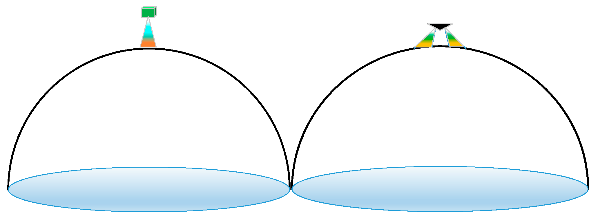
First, we compare the antenna observation modes of the current GNSS-R missions. TDS-1 (TechDemoSat-1), which is the precursor of the CYGNSS mission, has only one nadir antenna that uses a fixed array of four flared spiral elements. However, each micro-satellite in the CYGNSS constellation has two tilted antenna elements.
Figure 1 shows the TDS-1 and CYGNSS nadir antenna observation modes. Obviously, the two-antenna mode should be selected because it can receive more GNSS reflected signals than the single antenna mode when the same instruments are used. Additionally, in the processing of GNSS-R data, the transformation between spatial location on the Earth surface and location in the DDM has ambiguities outside the specular region [
41]. When two antennae face different directions, to some extent, they can receive and distinguish the signals reflected from locations in different direction on the Earth surface. It will make a positive impact on the solution of the typical ambiguity problem for GNSS-R.
From
Figure 1, the reflecting ground coverage for the two kinds of antenna modes are both finite, and are limited by the antenna beamwidth. Using TDS-1 as an example, the beamwidths are 34° × 35° at GPS L1, with a peak gain of 13.8 dBi, and 49° × 41° at GPS L2, with a peak gain of 10.8 dBi [
23]. However, no files have been released that contain the definitive beamwidths of the CYGNSS antennae. Therefore, in this paper, the beamwidth angles used for the GNSS-R LEO nadir antennae are the same as those of TDS-1.
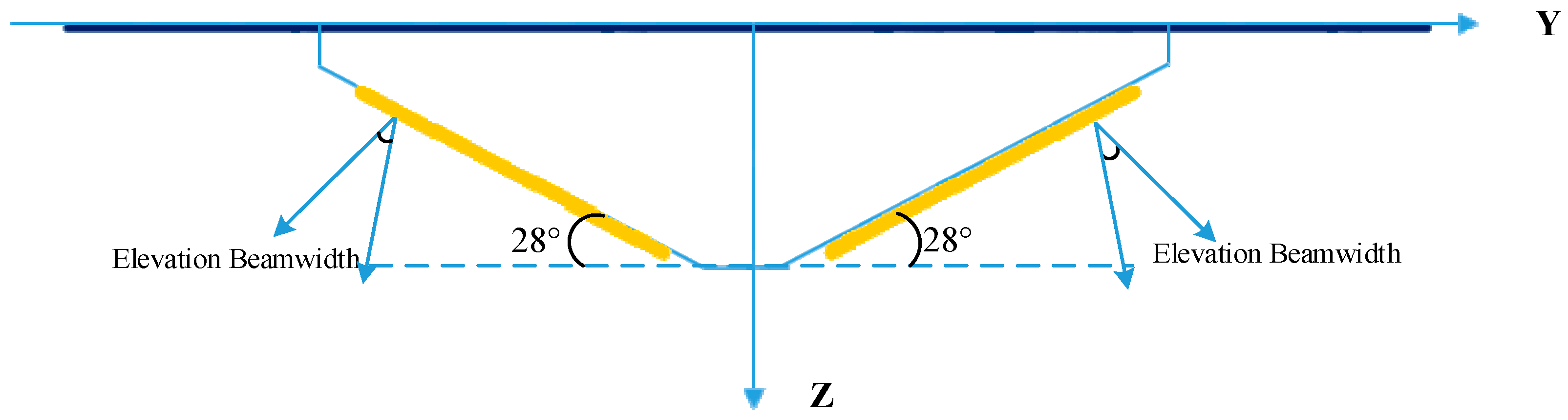
Figure 2 shows a schematic view of a CYGNSS microsatellite and its double nadir antennae. In
Figure 2 and
Figure 3, the +X and +Z axes point in the directions of flight and nadir, respectively. The +Y axis points towards the normal of the orbit plane and the orientations follow the right-hand rule. The antennae are off-pointing from the nadir by 28°. At the GPS L1 frequency, the elevation beamwidth is 34° and the azimuth beamwidth is 35°. The corresponding values at the GPS L2 frequency are 49° and 41°, respectively.
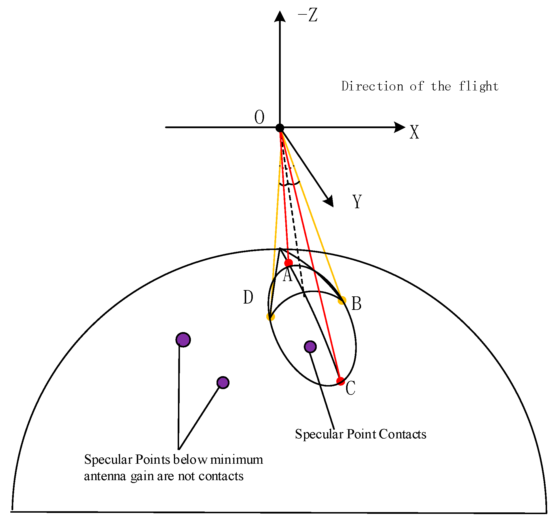
Figure 3 shows the available observation area for a single CYGNSS LHCP antenna on the Earth’s surface. The specular points that are located within the green area can be contacted, while the points that lie outside the green area cannot be contacted. The next subsection will be devoted to the design of a method for removal of the uncontacted specular reflections and selection of the available GNSS satellites; the reflected signals from these satellites can be received by the LEO observatory.
2.4. Selection of the Available Reflected Signals
We propose a three-step method for selection of the available GNSS reflected signals. (1) The potentially available GNSS satellites are selected for each LEO satellite; (2) the locations of the specular reflection points between the LEO and GNSS satellites are computed; (3) the specular reflection points that lie below the minimum antenna gain are removed.
In the processing of both ground-based and airborne GNSS-R measurements, we can simply select the available satellites based on the cutoff elevation because the direct signals can be deemed to be parallel with the reflected signals. However, the reflected points are very far away from the receivers in the spaceborne case, so that the views of the two signals are no longer in parallel. Here, we present a new method for selection of the available GNSS satellites.
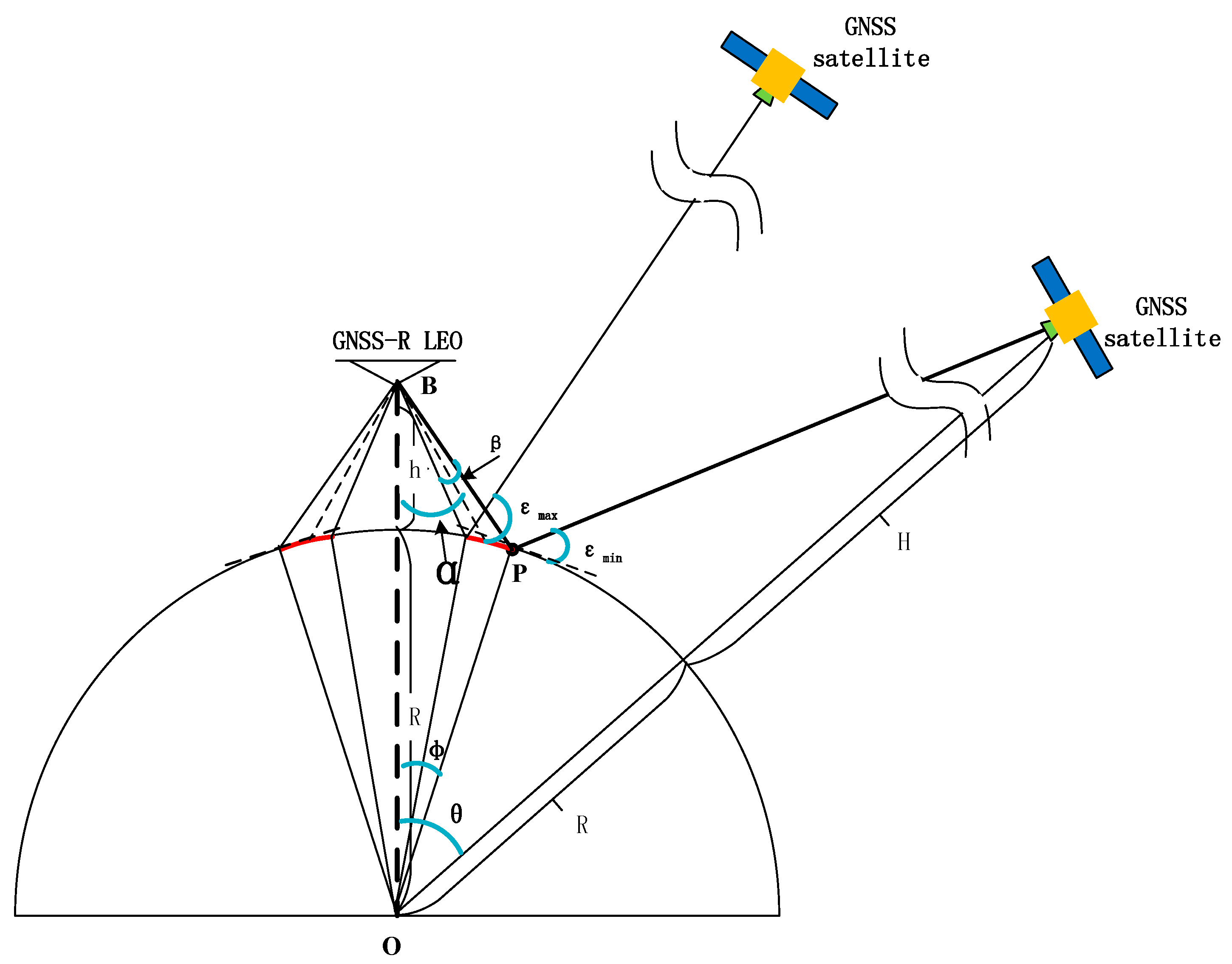
Figure 4 shows the geometrical relationships among the antenna face direction (
), the elevation beamwidth (
), the minimum elevation angle (
), the maximum elevation angle (
), the geocentric angle between the LEO and the specular reflected point (
), and the geocentric angle between the GNSS satellite and the LEO
. In
Figure 4, point O represents the center of the Earth; point P is the specular reflection point; point B is the location of the receiver antenna;
R is the Earth’s mean radius;
h is the orbit height of the GNSS-R LEO observatory, and
H is the GNSS satellite’s orbit altitude. The red arcs indicate the profiles of the reflecting ground coverage. When the specular points are located at the edges of these red arcs, there are minimum and maximum elevations. These minimum and maximum elevations can be derived using the following equations.
The minimum elevations are 40.31° and 31.18° at L1 and L2, respectively, while the maximum elevations are 78.13° and 86.23° at L1 and L2, respectively.
After the minimum elevation with respect to the specular points is obtained, based on the sine theorem within the triangle that is formed by the LEO, the Earth’s center and the specular point, Equation (3) can be given as follows.
can then be calculated using Equation (3). Subsequently,
can be derived based on Equation (4).
In Equation (4), because the minimum and maximum angles
have already been determined, the value of
is dependent on
H and
. Therefore,
will change with the altitudes of the different GNSS satellites, which range from 19,100 km to 35,900 km.
Table 3 lists the values of
H and
for the different types of GNSS satellites. We can then select the available GNSS satellites based on their geocentric angles at different epochs.
After the appropriate GNSS satellites have been selected, the locations of the reflections can then be determined using the method that was proposed by Wagner and Klokočník [
27]. The equations of computing the latitude and longitude of a specific specular reflected point according to the geometry shown in
Figure 4 are provided in this subsection. The locations of specular reflected points can be computed using Equations (5) and (6).
where
and
are the geodetic latitude and longitude of the LEO, respectively;
and
are the geodetic latitude and longitude of the GNSS satellite, respectively;
and
are the geodetic latitude and longitude of the reflected point, respectively.
After computation of the locations of the specular reflection points, we must remove the specular points that are below the minimum antenna gain. We propose a method based on the use of the azimuths and elevations of the vectors between the reflections and the LEO satellites in the body-fixed coordinate system to select the available reflections. We can obtain the azimuth and elevation ranges at both L1 and L2 using the beamwidths and face directions of the antennae.
Based on the geometry shown in
Figure 4, the elevation angle range can easily be computed to be
. However, to obtain the azimuth range, which is the angle between the
x-axis vector and the reflection, the vectors OD and OB in the body-fixed coordinate system shown in
Figure 3 must be determined. The following characteristics of OD and OB can help us to solve for the values of their unit vectors. Both vectors OD and OB lie perpendicular to the antenna axis
and the angle between this axis and the normal vector of the panel
is
, where
is the elevation beamwidth. The unit vectors of OB and OD can be set to
. The following three equations are therefore derived:
The solutions for are , and .
From the solutions to Equation (7) and the geometry, the azimuths of OB and OD in the body-fixed coordinate system are determined to be 123.07° and 56.93°, respectively, at the L1 frequency, while the corresponding angles are 51.47° and 128.53°, respectively, at the L2 frequency. After the elevation and azimuth ranges are computed, the available specular reflection points can then be selected.
2.5. The Revisit Time Computation Principle
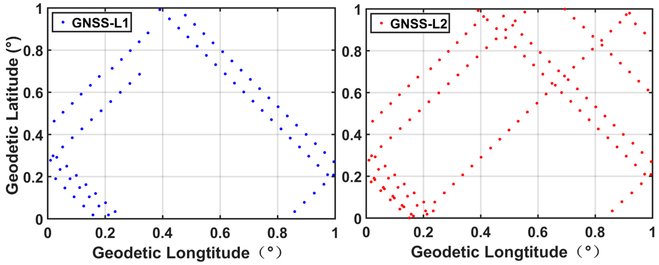
To assess the observation capacity of a future GNSS-R constellation that is compatible with the four GNSS systems, the spatial and temporal resolutions of the specular reflection points must be computed. Because the reflected points are located using the precise coordinates from the GNSS and the LEO satellites, it is difficult to find an analytical algorithm that can calculate the temporal resolution like that for monostatic remote sensing satellites. However, the reflections also form continuous ground tracks on the Earth’s surface that look like the arcs and passes shown in
Figure 5.
Figure 5 shows the reflection point distribution in a single 1° × 1° bin during 48 h period for a 1° × 1° bin at GPS L1 frequency (left) and GPS L2 frequency (right) when eight GNSS-R LEO satellites and 119 GNSS satellites are used.
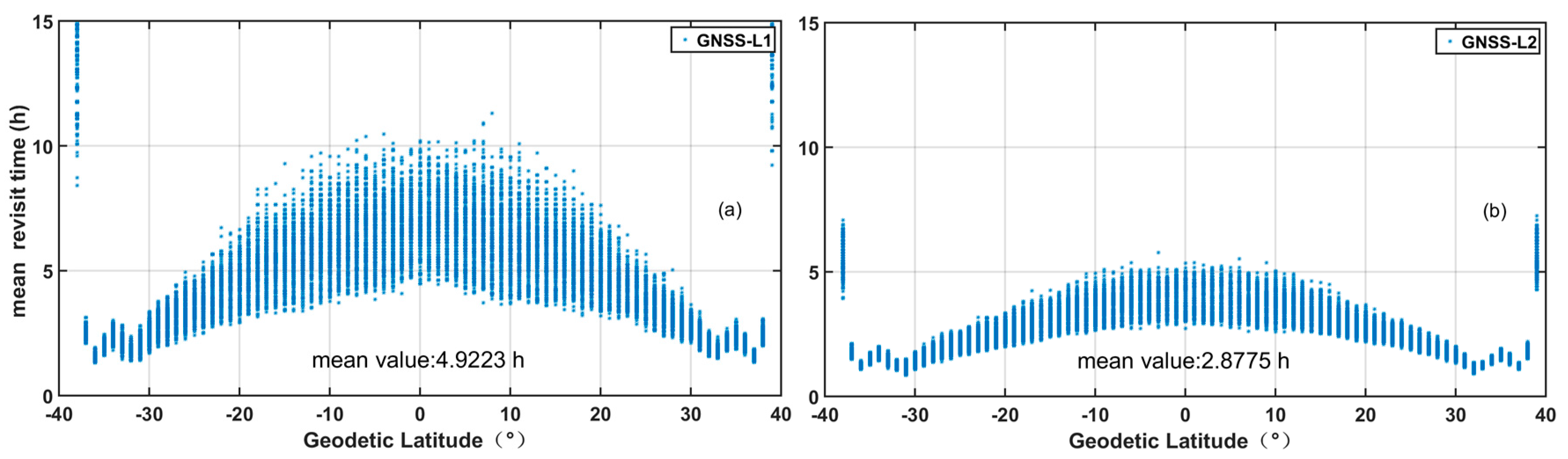
The interval between successive passes in one bin, i.e., the revisit time, is regarded as an index of the temporal resolution. Every track on the ground stands for a pass, and the period divided by the number of tracks is mean revisit time. The mean revisit time is an important criterion that is used to evaluate the GNSS-R LEO constellation. For instance, we can find that there are 8 ground tracks and 13 ground tracks during 48 h in
Figure 5 (left) and
Figure 5 (right), respectively. So, the values of mean revisit time in
Figure 5 (left) and
Figure 5 (right) are 6 h and 3.69 h, respectively. Here, the Earth’s surface is divided into 1° × 1° bins and we have developed a program that can compute the mean revisit time for each bin.
4. Discussion
The GNSS-R of the future will feature the combination of GPS, BDS, GLONASS and GALILEO, and high spatiotemporal resolutions. In order to evaluate observation capacity of a multi-GNSS-R LEO constellation quantitatively, detailed comparisons were made between the case where the four GNSS systems were available and the case where only the GPS system was used at the L1 and L2 frequencies in this work. And other useful advice and hints on how to design certain criteria for future spaceborne GNSS-R instruments and constellations are given in this paper. Additionally, this research not only advances our understanding of the observation capacity of the proposed four-system GNSS-R but also presents some appropriate simulation methods and results.
Pervious researchers had also stated some results about the GNSS-R spatial and temporal resolutions, but early simulations were conducted based on GPS and one LEO satellite, and other late results are lack of details [
24,
25,
26,
27,
28,
31]. Here, we describe the simulation and analysis methods, as well as the parameters’ values, used in this paper, and conduct the experiments using 119 GNSS satellites and 8 LEO satellites. However, the spatial and temporal resolutions of GNSS-R missions vary with several parameters, such as constellation constructions, antennae beamwidths and observation modes. The ones who design GNSS-R missions with different targets can use the methods given in this paper to recompute the observation resolutions.
Evaluation of the spatial and temporal resolutions of the GNSS-R reflections is very important for different types of GNSS-R missions with different objectives. Among the current applications of the GNSS-R techniques, monitoring of sea surface winds is the most mature. Other potential applications include ocean and ice altimetry. For the investigation of cyclone generation processes, we suggest that one or two of the GNSS-R LEO satellites should be put into orbit at a 20° inclination because 87% of hurricanes form no farther away than 20° north or south [
42,
43]. However, for ocean sea surface altimetry, the GNSS-R observatories should be inclined at 70° to cover the high latitude sea surfaces and the number of observatories required will be less than that required for monitoring of the sea surface winds.
In this study, the results are obtain by using simulated data, including parts of GNSS constellations and the GNSS-R LEO constellation. It is impractical for us to perform an officially sensitivity/uncertainty assessments on the simulated orbits. So, there are inevitable potential errors that might be associated with these constellations.
Two or three years later, the four main GNSS systems will be fully operational, and their precise orbits will be released. If the precise orbits and other related parameters of a certain GNSS-R LEO constellation are provided, the methods presented in this paper can be used to evaluate the performance of that GNSS-R system with higher accuracy and authoritative.
In addition, we assess the spatial resolutions of GNSS-R using the numbers of reflections in different 1° × 1° bins simply. However, the observed scene for one reflection can be divided into several areas with smaller size [
22]. So, the spatial resolutions also depend on the algorithm of GNSS-R data processing. A deeper analysis on the spatial resolutions based on different algorithms can be achieved in future work.
5. Conclusions
The initial motivation of this work was to evaluate the observation capacity of a near-future GNSS-R LEO constellation based on simulated orbits and reflections when all four GNSS systems are available after 2020. In this paper, we propose a strategy for construction of a multi-GNSS-R system that includes 119 GNSS satellites and eight LEO GNSS-R observatories with two nadir GNSS LHCP antennae apiece, along with a three-step method to select the available GNSS reflection signals. In addition, a method for calculation of the revisit time for the GNSS-R specular reflections is presented. The results of these simulations have helped us to analyze and evaluate the performance of future four-system spaceborne GNSS-R missions quantitatively. Detailed comparisons were made between the case where the four GNSS systems were available and the case where only the GPS system was used at the L1 and L2 frequencies.
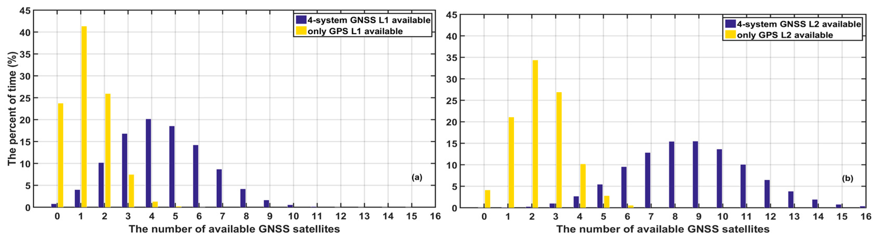
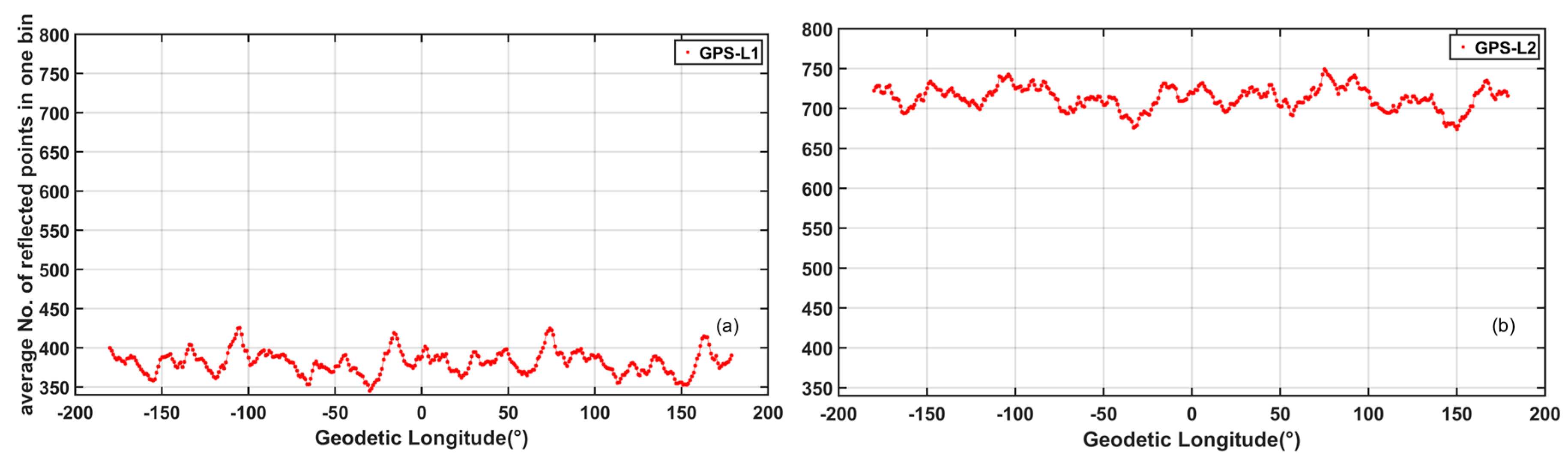
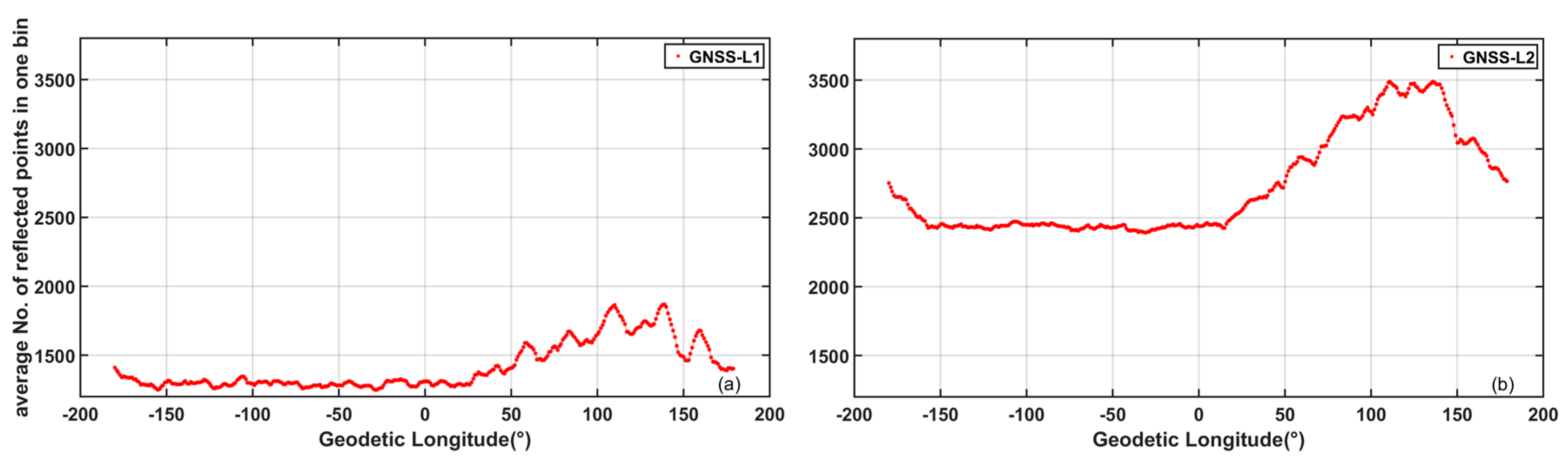
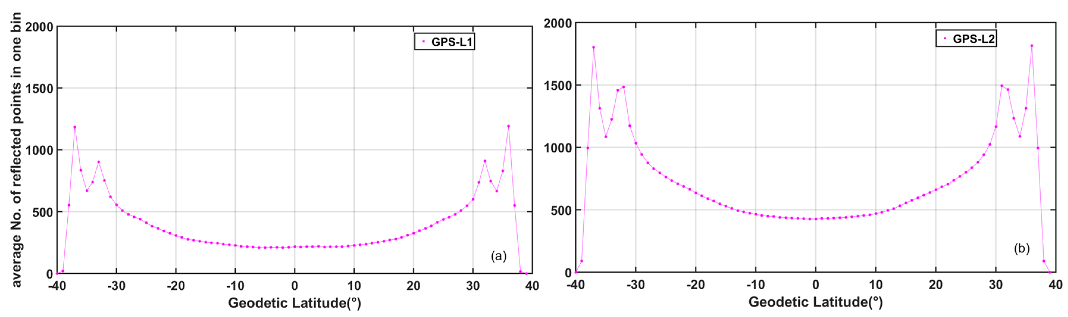
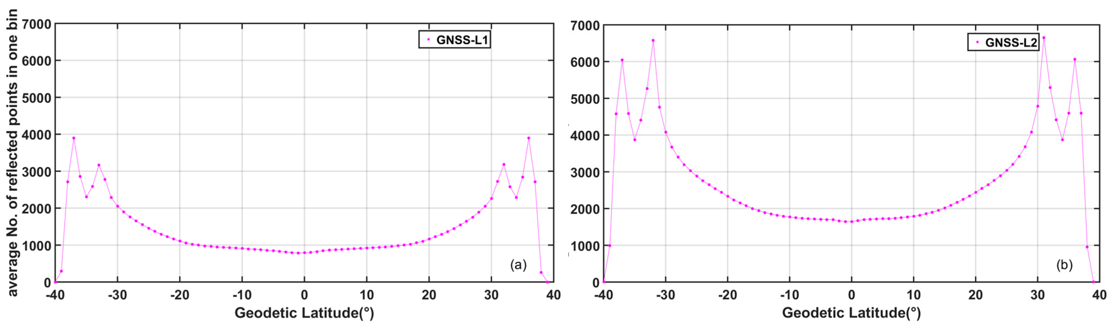
In the case of the four-system GNSS-R, a single observatory can track up to 10 and 16 parallel specular reflections at the GPS L1 and L2 frequencies, respectively. However, in the GPS-R case, a given GNSS-R LEO satellite can only track up to four and six parallel specular reflections at the GPS L1 and L2 frequencies, respectively. In addition, 1.2 GPS-only reflections and 4.5 four-system GNSS reflections can be received at L1 on average, while the corresponding values at L2 are 2.3 and 8.7 because of its wider beamwidth. We therefore propose that future spaceborne GNSS-R instruments should have wider beamwidths and the ability to receive more signals from different GNSS systems to allow the system to provide more available reflections.
Larger numbers of observations would improve the spatiotemporal sampling over that of current spaceborne missions. The number of multi-GNSS-R reflections in a single 1° × 1° grid is several times the corresponding number of GPS-only reflections. The spatial density of the specular reflections in the Asia-Pacific region is higher than that in other areas at the same latitude because of the locations of the Chinese BDS GEO and IGSO satellites. Additionally, the numbers of reflections around are two to four times higher than those in other areas because of the orbit inclinations of the LEO GNSS-R observatories. When compared with the GPS-R case, the mean revisit times will be reduced by approximately three times when the satellites from all four GNSS systems are used. Overall, the number of available GNSS illuminators, the distribution of the GNSS satellites and the inclinations of the LEO satellites are closely related to the spatiotemporal resolution of GNSS-R.
For a specific mission design, the parameters of the instrument and orbits will different from those presented in this paper. In future work, several possible LEO constellations for different targets will be constructed and simulations will be conducted to assess the performances of a planned GNSS-R mission.


