Multi-Temporal Analysis of Forestry and Coastal Environments Using UASs

 , , , , ,
Abstract
:
1. Introduction
2. Background
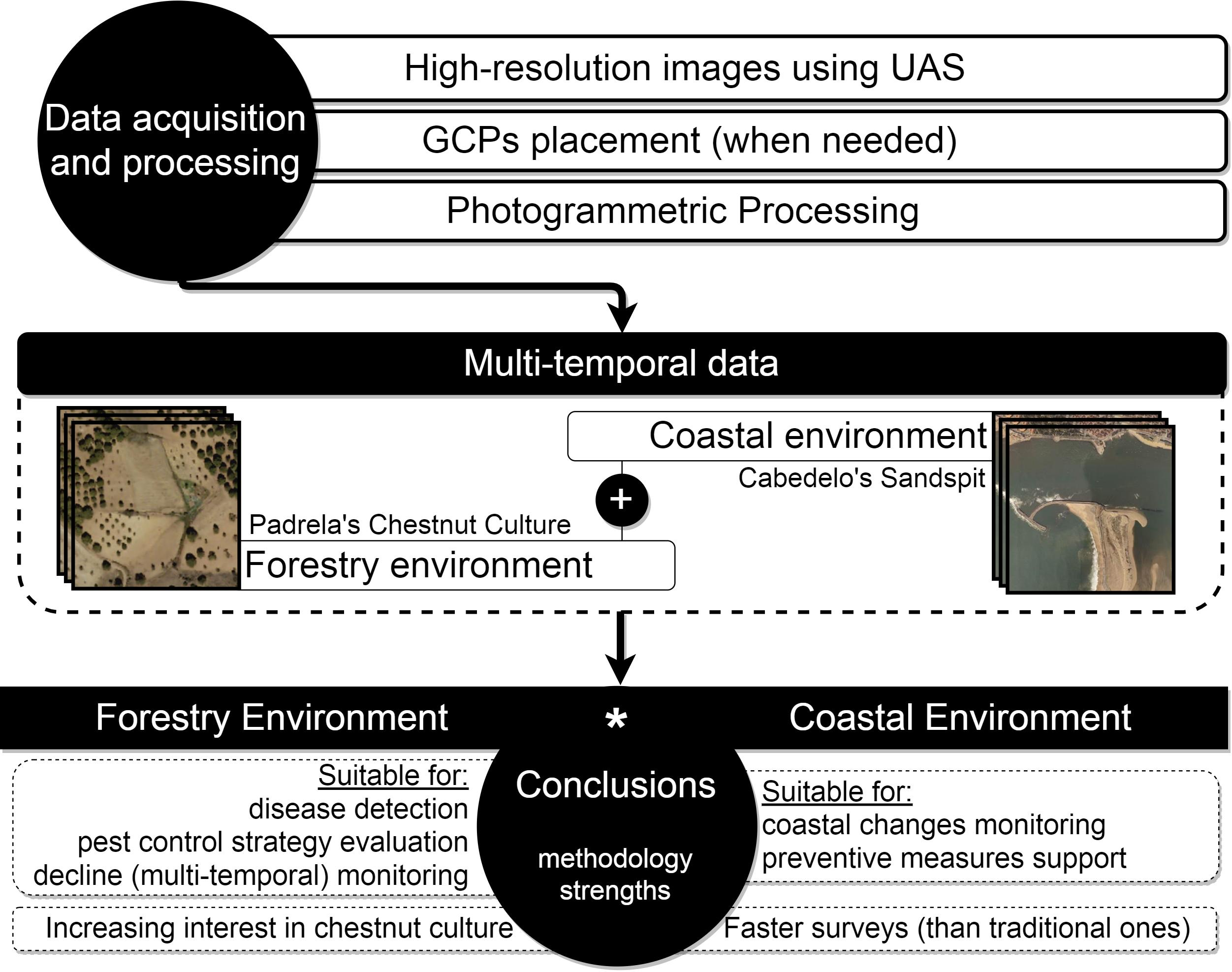
3. Methodology
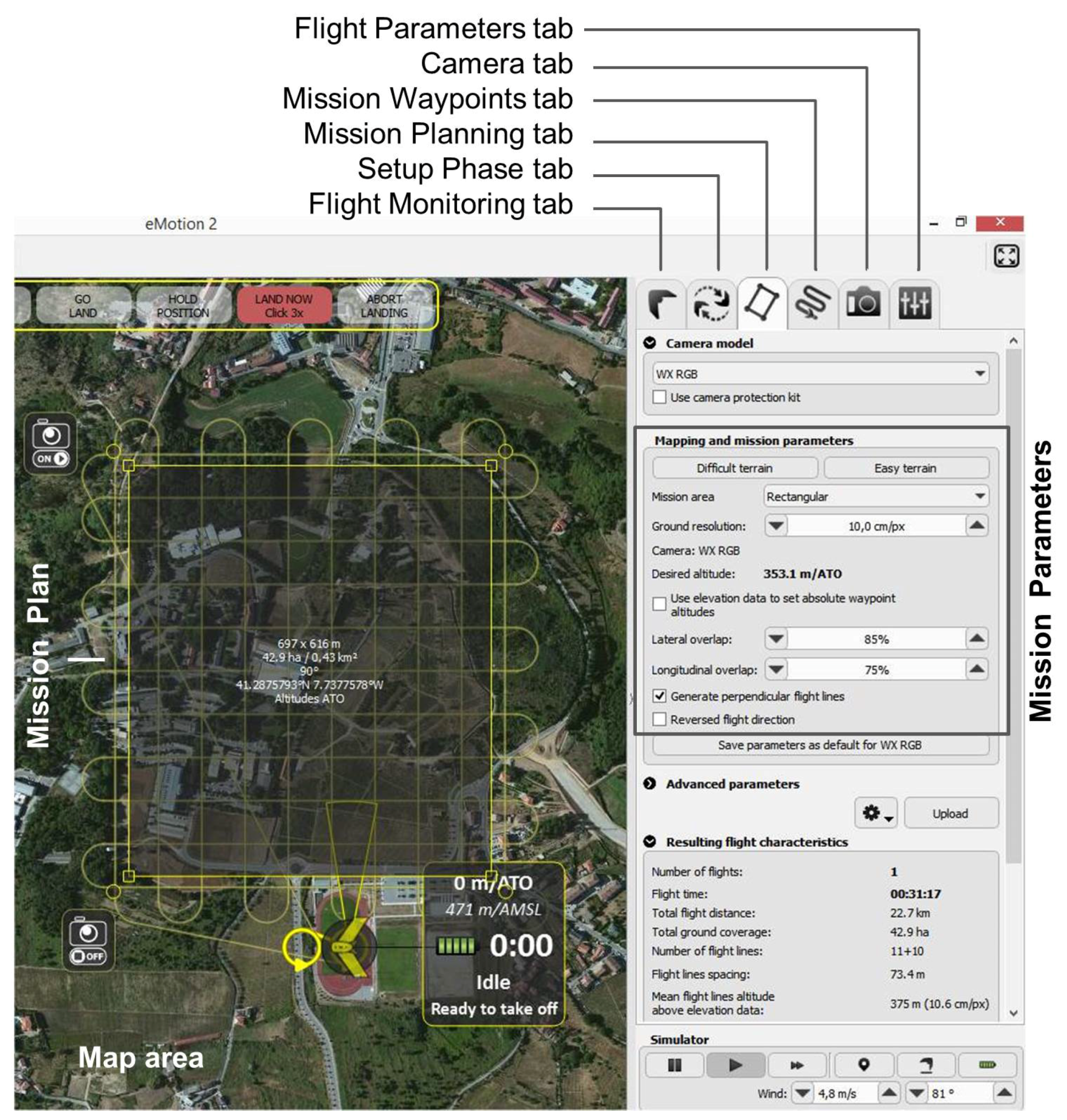
3.1. Data Collection
3.2. Data Processing
4. Case Studies
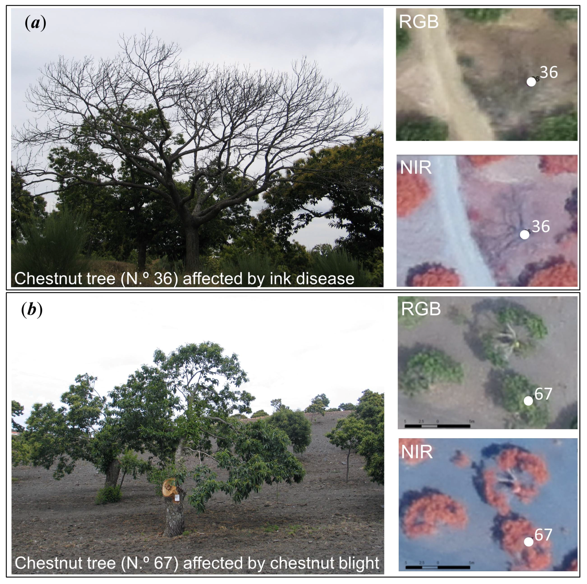
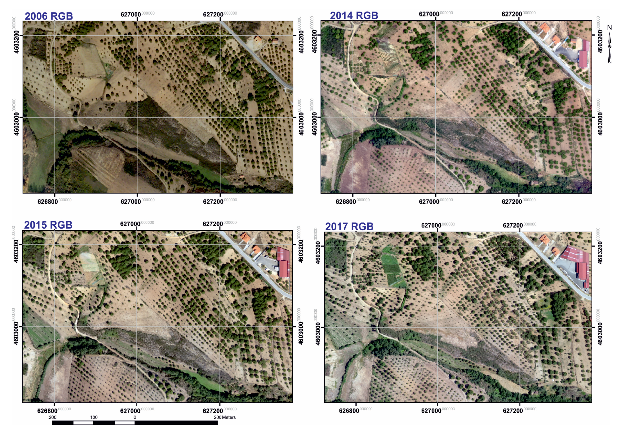
4.1. Chestnut Health Monitoring
4.1.1. Considerations about Surveys of Chestnut Trees
- CG—Chestnut growth (%)
- CI—Canopy cover index in 2006
- CI—Canopy cover index in 2014
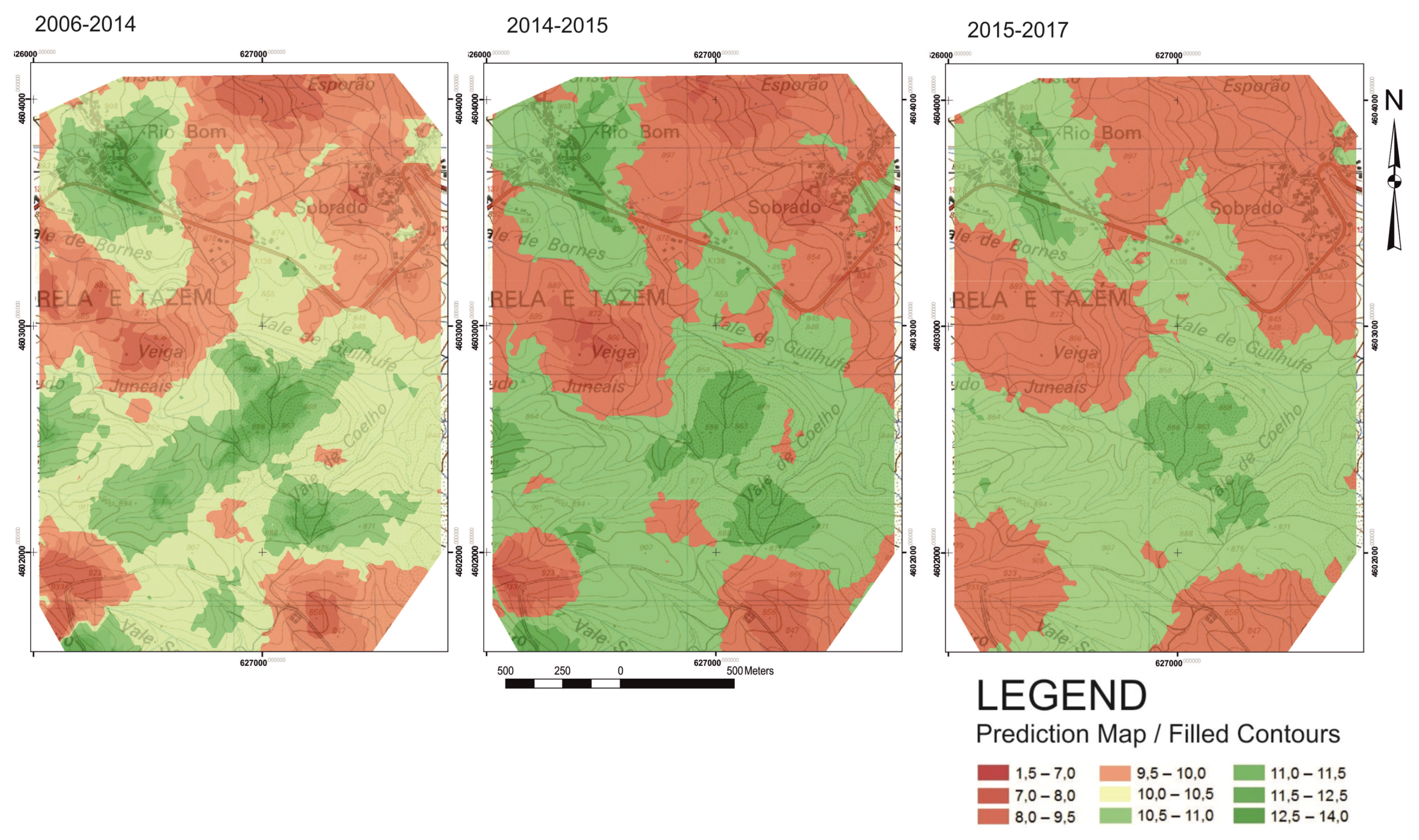
4.1.2. Results and Discussion
- detecting chestnut ink disease symptoms [84];
- monitoring tree canopy cover decline by means of multi-temporal analysis (assess chestnut blight presence);
- providing the means for evaluating gall wasp biological control strategy effectiveness.
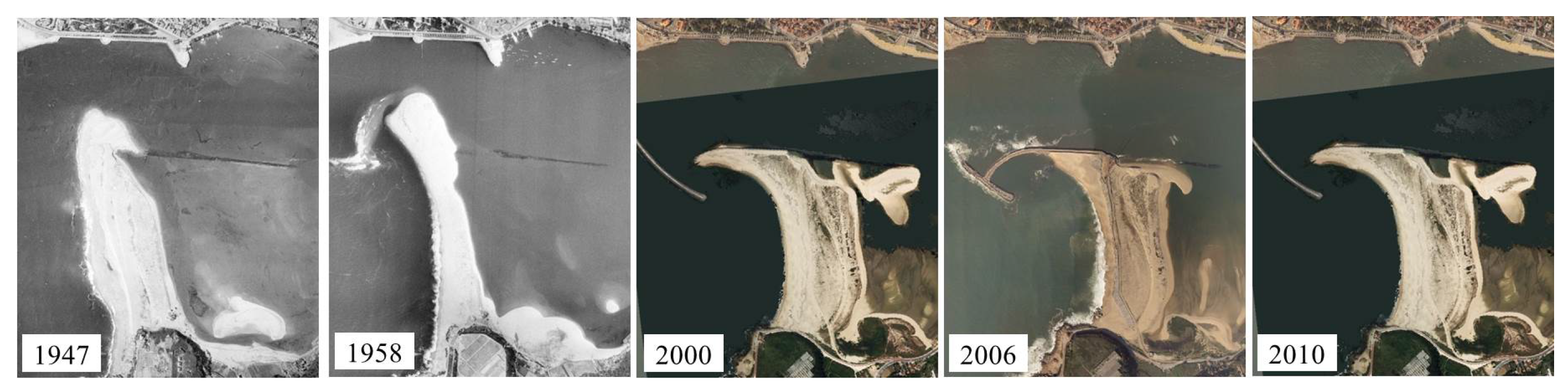
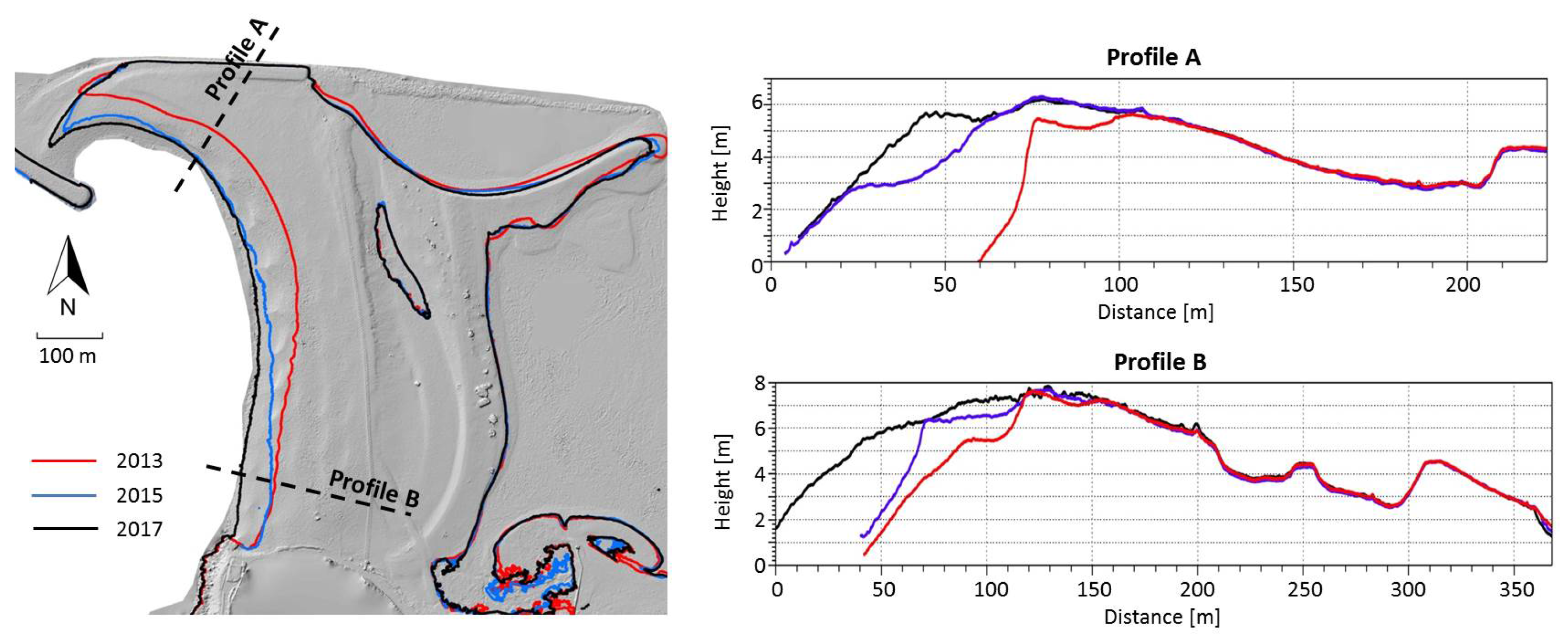
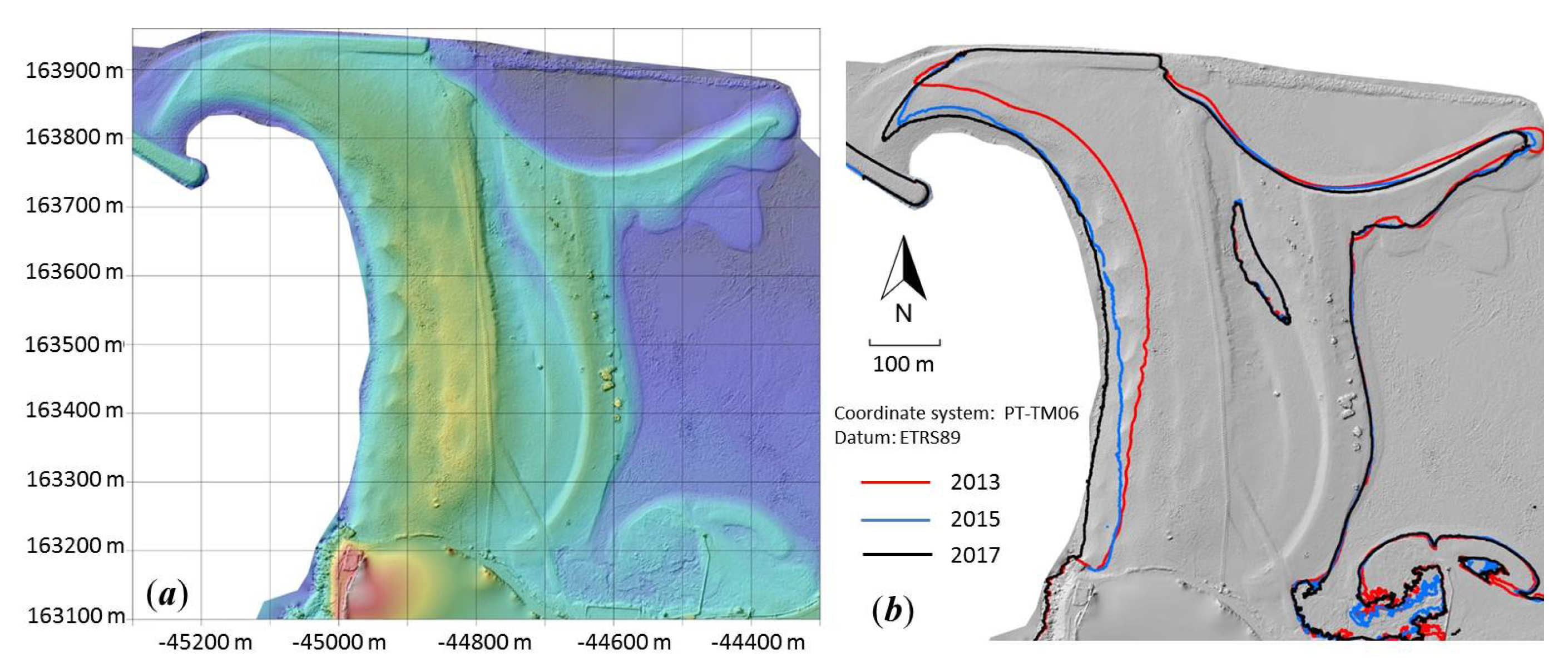
4.2. Cabedelo Sandspit Variation Assessment
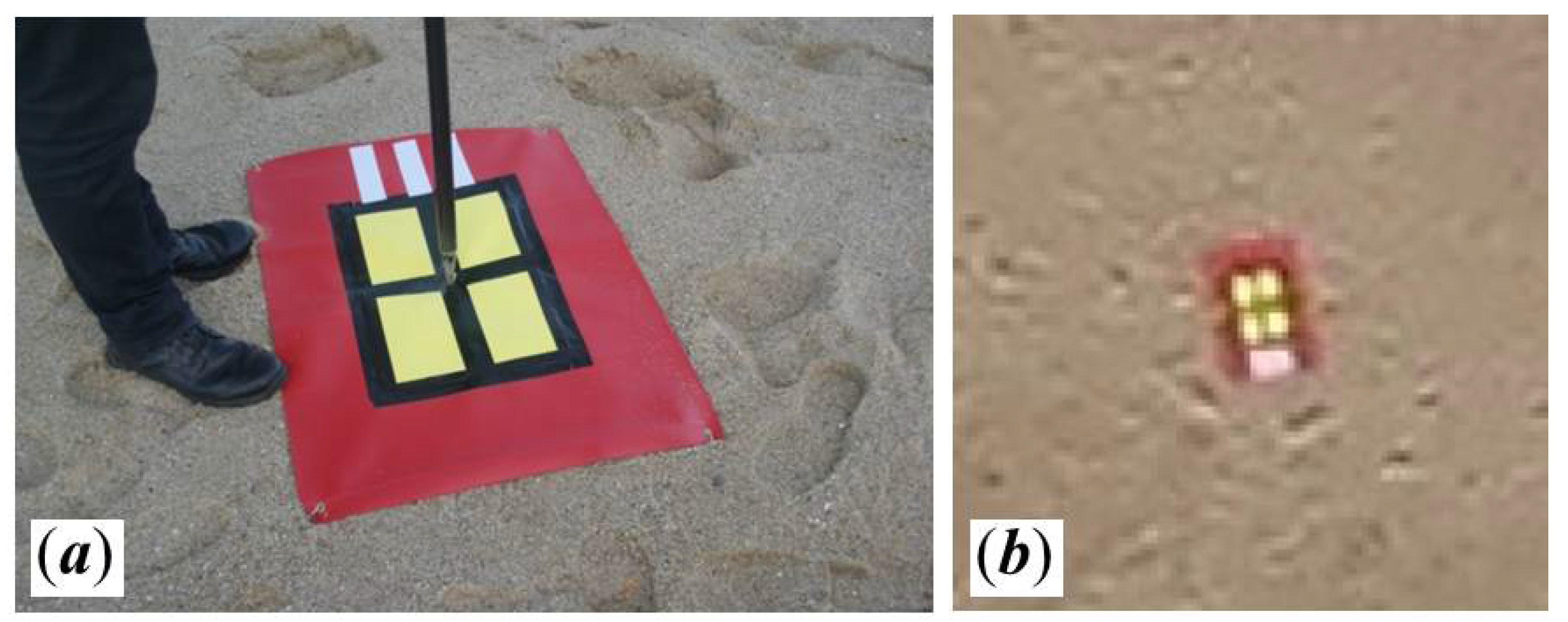
4.2.1. Considerations about Surveys in Sand Areas
4.2.2. Results and Discussion
5. Conclusions
Acknowledgments
Author Contributions
Conflicts of Interest
References
- Ermacora, G.; Toma, A.; Rosa, S.; Bona, B.; Chiaberge, M.; Silvagni, M.; Gaspardone, M.; Antonini, R. A Cloud Based Service for Management and Planning of Autonomous UAV Missions in Smart City Scenarios. In Proceedings of the Modelling and Simulation for Autonomous Systems: First International Workshop (MESAS), Rome, Italy, 5–6 May 2014; Hodicky, J., Ed.; Revised Selected Papers. Springer International Publishing: Cham, Switzerland, 2014; pp. 20–26. [Google Scholar]
- Oleire-Oltmanns, S.; Marzolff, I.; Peter, D.K.; Ries, B.J. Unmanned Aerial Vehicle (UAV) for Monitoring Soil Erosion in Morocco. Remote Sens. 2012, 4, 3390–3416. [Google Scholar] [CrossRef]
- Jenkins, D.; Vasigh, B. The Economic Impact of Unmanned Aircraft Systems Integration in the United States. Available online: http://www.auvsi.org/auvsiresources/economicreport (accessed on 23 December 2017).
- Pádua, L.; Vanko, J.; Hruška, J.; Adão, T.; Sousa, J.J.; Peres, E.; Morais, R. UAS, sensors, and data processing in agroforestry: A review towards practical applications. Int. J. Remote Sens. 2017, 38, 2349–2391. [Google Scholar] [CrossRef]
- Matese, A.; Toscano, P.; Di Gennaro, S.F.; Genesio, L.; Vaccari, F.P.; Primicerio, J.; Belli, C.; Zaldei, A.; Bianconi, R.; Gioli, B. Intercomparison of UAV, aircraft and satellite remote sensing platforms for precision viticulture. Remote Sens. 2015, 7, 2971–2990. [Google Scholar] [CrossRef]
- Atzberger, C. Advances in Remote Sensing of Agriculture: Context Description, Existing Operational Monitoring Systems and Major Information Needs. Remote Sens. 2013, 5, 949–981. [Google Scholar] [CrossRef]
- Mirijovský, J.; Langhammer, J. Multitemporal Monitoring of the Morphodynamics of a Mid-Mountain Stream Using UAS Photogrammetry. Remote Sens. 2015, 7, 8586–8609. [Google Scholar] [CrossRef]
- Tanteri, L.; Rossi, G.; Tofani, V.; Vannocci, P.; Moretti, S.; Casagli, N. Multitemporal UAV Survey for Mass Movement Detection and Monitoring. In Advancing Culture of Living with Landslides: Volume 2 Advances in Landslide Science; Mikos, M., Tiwari, B., Yin, Y., Sassa, K., Eds.; Springer International Publishing: Cham, Switzerland, 2017; pp. 153–161. [Google Scholar]
- Jomaa, I.; Auda, Y.; Abi Saleh, B.; Hamzé, M.; Safi, S. Landscape spatial dynamics over 38 years under natural and anthropogenic pressures in Mount Lebanon. Landsc. Urban Plan. 2008, 87, 67–75. [Google Scholar] [CrossRef]
- Niethammer, U.; James, M.R.; Rothmund, S.; Travelletti, J.; Joswig, M. UAV-based Remote Sensing of the Super-Sauze Landslide: Evaluation and Results. Eng. Geol. 2012, 128, 2–11. [Google Scholar] [CrossRef]
- Cho, J.; Lim, G.; Biobaku, T.; Kim, S.; Parsaei, H. Safety and Security Management with Unmanned Aerial Vehicle (UAV) in Oil and Gas Industry. Procedia Manuf. 2015, 3, 1343–1349. [Google Scholar] [CrossRef]
- Dooly, G.; Omerdic, E.; Coleman, J.; Miller, L.; Kaknjo, A.; Hayes, J.; Braga, J.; Ferreira, F.; Conlon, H.; Barry, H.; et al. Unmanned Vehicles for Maritime Spill Response Case Study: Exercise Cathach. Mar. Pollut. Bull. 2016, 110, 528–538. [Google Scholar] [CrossRef] [PubMed]
- Funaki, M.; Higashino, S.I.; Sakanaka, S.; Iwata, N.; Nakamura, N.; Hirasawa, N.; Obara, N.; Kuwabara, M. Small Unmanned Aerial Vehicles for Aeromagnetic Surveys and Their Flights in the South Shetland Islands, Antarctica. Polar Sci. 2014, 8, 342–356. [Google Scholar] [CrossRef]
- Turner, I.L.; Harley, M.D.; Drummond, C.D. UAVs for Coastal Surveying. Coast. Eng. 2016, 114, 19–24. [Google Scholar] [CrossRef]
- Candiago, S.; Remondino, F.; De Giglio, M.; Dubbini, M.; Gattelli, M. Evaluating Multispectral Images and Vegetation Indices for Precision Farming Applications from UAV Images. Remote Sens. 2015, 7, 4026–4047. [Google Scholar] [CrossRef]
- Lisein, J.; Pierrot-Deseilligny, M.; Bonnet, S.; Lejeune, P. A Photogrammetric Workflow for the Creation of a Forest Canopy Height Model from Small Unmanned Aerial System Imagery. Forests 2013, 4, 922–944. [Google Scholar] [CrossRef]
- Colomina, I.; Molina, P. Unmanned Aerial Systems for Photogrammetry and Remote Sensing: A Review. ISPRS J. Photogramm. Remote Sens. 2014, 92, 79–97. [Google Scholar] [CrossRef]
- Jia, Y.; Su, Z.; Shen, W.; Yuan, J.; Xu, Z. UAV Remote Sensing Image Mosaic and Its Application in Agriculture. Int. J. Smart Home 2016, 10, 159–170. [Google Scholar] [CrossRef]
- Prabhakar, M.; Prasad, Y.G.; Rao, M.N. Remote Sensing of Biotic Stress in Crop Plants and Its Applications for Pest Management. In Crop Stress and Its Management: Perspectives and Strategies; Venkateswarlu, B., Shanker, A.K., Shanker, C., Maheswari, M., Eds.; Springer: Dordrecht, The Netherlands, 2012; pp. 517–545. [Google Scholar]
- De Estatística, I.N. Estatísticas Agrícolas; Instituto Nacional de Estatística Statistics Portugal: Lisbon, Portugal, 2016. [Google Scholar]
- Chen, J.S.; Li, L.; Wang, J.Y.; Barry, D.A.; Sheng, X.F.; Gu, W.Z.; Zhao, X.; Chen, L. Water resources: Groundwater maintains dune landscape. Nature 2004, 432, 459–460. [Google Scholar] [CrossRef] [PubMed]
- Mancini, F.; Dubbini, M.; Gattelli, M.; Stecchi, F.; Fabbri, S.; Gabbianelli, G. Using Unmanned Aerial Vehicles (UAV) for High-Resolution Reconstruction of Topography: The Structure from Motion Approach on Coastal Environments. Remote Sens. 2013, 5, 6880–6898. [Google Scholar] [CrossRef] [Green Version]
- Pettorelli, N.; Laurance, W.F.; O’Brien, T.G.; Wegmann, M.; Nagendra, H.; Turner, W. Satellite remote sensing for applied ecologists: Opportunities and challenges. J. Appl. Ecol. 2014, 51, 839–848. [Google Scholar] [CrossRef]
- Ponti, M.P. Segmentation of Low-Cost Remote Sensing Images Combining Vegetation Indices and Mean Shift. IEEE Geosci. Remote Sens. Lett. 2013, 10, 67–70. [Google Scholar] [CrossRef]
- Zhang, C.; Kovacs, J.M. The Application of Small Unmanned Aerial Systems for Precision Agriculture: A Review. Precis. Agric. 2012, 13, 693–712. [Google Scholar] [CrossRef]
- Whitehead, K.; Hugenholtz, C.H. Remote sensing of the environment with small unmanned aircraft systems (UASs), part 1: A review of progress and challenges. J. Unman. Veh. Syst. 2014, 2, 69–85. [Google Scholar] [CrossRef]
- Fraser, R.H.; Olthof, I.; Lantz, T.C.; Schmitt, C. UAV photogrammetry for mapping vegetation in the low-Arctic. Arct. Sci. 2016, 2, 79–102. [Google Scholar] [CrossRef]
- Gevaert, C.M.; Persello, C.; Sliuzas, R.; Vosselman, G. Informal settlement classification using point-cloud and image-based features from UAV data. ISPRS J. Photogramm. Remote Sens. 2017, 125, 225–236. [Google Scholar] [CrossRef]
- Suomalainen, J.; Anders, N.; Iqbal, S.; Roerink, G.; Franke, J.; Wenting, P.; Hünniger, D.; Bartholomeus, H.; Becker, R.; Kooistra, L. A Lightweight Hyperspectral Mapping System and Photogrammetric Processing Chain for Unmanned Aerial Vehicles. Remote Sens. 2014, 6, 11013–11030. [Google Scholar] [CrossRef]
- Xie, Y.; Sha, Z.; Yu, M. Remote sensing imagery in vegetation mapping: A review. J. Plant Ecol. 2008, 1, 9–23. [Google Scholar] [CrossRef]
- Laliberte, A.S.; Winters, C.; Rango, A. UAS remote sensing missions for rangeland applications. Geocarto Int. 2011, 26, 141–156. [Google Scholar] [CrossRef]
- Puliti, S.; Orka, O.H.; Gobakken, T.; Næsset, E. Inventory of Small Forest Areas Using an Unmanned Aerial System. Remote Sens. 2015, 7, 9632–9654. [Google Scholar] [CrossRef] [Green Version]
- Garcia-Torres, L.; Caballero-Novella, J.J.; Gómez-Candón, D.; De-Castro, A.I. Semi-Automatic Normalization of Multitemporal Remote Images Based on Vegetative Pseudo-Invariant Features. PLoS ONE 2014, 9, e91275. [Google Scholar] [CrossRef] [PubMed]
- Jha, A.R. Theory, Design, and Applications of Unmanned Aerial Vehicles; CRC Press: Boca Raton, FL, USA, 2016. [Google Scholar]
- Watts, A.C.; Ambrosia, V.G.; Hinkley, E.A. Unmanned Aircraft Systems in Remote Sensing and Scientific Research: Classification and Considerations of Use. Remote Sens. 2012, 4, 1671–1692. [Google Scholar] [CrossRef]
- Aber, J.S.; Marzolff, I.; Ries, J. Small-Format Aerial Photography: Principles, Techniques and Geoscience Applications; Elsevier Science: Amsterdam, The Netherlands, 2010. [Google Scholar]
- Gutiérrez, P.A.; López-Granados, F.; Peña-Barragán, J.M.; Jurado-Expósito, M.; Hervás-Martínez, C. Logistic regression product-unit neural networks for mapping Ridolfia segetum infestations in sunflower crop using multitemporal remote sensed data. Comput. Electron. Agric. 2008, 64, 293–306. [Google Scholar] [CrossRef]
- Lan, Y.; Huang, Y.; Martin, D.E.; Hoffmann, W.C. Development of an Airborne Remote Sensing System for Crop Pest Management: System Integration and Verification. Appl. Eng. Agric. 2009, 25, 607–615. [Google Scholar] [CrossRef]
- Fladeland, M.; Sumich, M.; Lobitz, B.; Kolyer, R.; Herlth, D.; Berthold, R.; McKinnon, D.; Monforton, L.; Brass, J.; Bland, G. The NASA SIERRA science demonstration programme and the role of small–medium unmanned aircraft for earth science investigations. Geocarto Int. 2011, 26, 157–163. [Google Scholar] [CrossRef]
- Primicerio, J.; Di Gennaro, S.F.; Fiorillo, E.; Genesio, L.; Lugato, E.; Matese, A.; Vaccari, F.P. A flexible unmanned aerial vehicle for precision agriculture. Precis. Agric. 2012, 13, 517–523. [Google Scholar] [CrossRef]
- Gonzalez-Dugo, V.; Zarco-Tejada, P.; Nicolás, E.; Nortes, P.A.; Alarcón, J.J.; Intrigliolo, D.S.; Fereres, E. Using high resolution UAV thermal imagery to assess the variability in the water status of five fruit tree species within a commercial orchard. Precis. Agric. 2013, 14, 660–678. [Google Scholar] [CrossRef]
- Tamminga, A.; Hugenholtz, C.; Eaton, B.; Lapointe, M. Hyperspatial Remote Sensing of Channel Reach Morphology and Hydraulic Fish Habitat Using an Unmanned Aerial Vehicle (UAV): A First Assessment in the Context of River Research and Management. River Res. Appl. 2015, 31, 379–391. [Google Scholar] [CrossRef]
- Turner, D.; Lucieer, A.; de Jong, M.S. Time Series Analysis of Landslide Dynamics Using an Unmanned Aerial Vehicle (UAV). Remote Sens. 2015, 7, 1736–1757. [Google Scholar] [CrossRef]
- Gonçalves, J.A.; Bastos, L.; Pinho, J.L.; Granja, H. Digital Aerial Photography to Monitor Changes in Coastal Areas Based on Direct Georeferencing. In Proceedings of the 5th EARSeL Workshop on Remote Sensing of the Coastal Zone, Prague, Czech Republic, 1–3 June 2011; pp. 1–10. [Google Scholar]
- Gonçalves, J.A.; Henriques, R. UAV Photogrammetry for Topographic Monitoring of Coastal Areas. ISPRS J. Photogramm. Remote Sens. 2015, 104, 101–111. [Google Scholar] [CrossRef]
- Drummond, C.D.; Harley, M.D.; Turner, I.L.; A Matheen, A.N.; Glamore, W.C. UAV Applications to Coastal Engineering. In Proceedings of the Australasian Coasts & Ports Conference, Auckland, New Zealand, 15–18 September 2015; pp. 267–272. [Google Scholar]
- Messinger, M.; Silman, M. Unmanned Aerial Vehicles for the Assessment and Monitoring of Environmental Contamination: An Example from Coal Ash Spills. Environ. Pollut. 2016, 218, 889–894. [Google Scholar] [CrossRef] [PubMed]
- Pereira, E.; Bencatel, R.; Correia, J.; Félix, L.; Gonçalves, G.; Morgado, J.; Sousa, J. Unmanned Air Vehicles for Coastal and Environmental Research. J. Coast. Res. 2009, II, 1557–1561. [Google Scholar]
- Hodgson, A.; Kelly, N.; Peel, D. Unmanned Aerial Vehicles (UAVs) for Surveying Marine Fauna: A Dugong Case Study. PLoS ONE 2013, 8, e79556. [Google Scholar] [CrossRef] [PubMed]
- Rhee, D.S.; Kim, Y.D.; Kang, B.; Kim, D. Applications of Unmanned Aerial Vehicles in Fluvial Remote Sensing: An Overview of Recent Achievements. KSCE J. Civ. Eng. 2017, 1–15. [Google Scholar] [CrossRef]
- Abdullahi, H.S.; Mahieddine, F.; Sheriff, R.E. Technology Impact on Agricultural Productivity: A Review of Precision Agriculture Using Unmanned Aerial Vehicles. In Proceedings of the Wireless and Satellite Systems: 7th International Conference on WiSATS, Bradford, UK, 6–7 July 2015; Pillai, P., Hu, Y.F., Otung, I., Giambene, G., Eds.; Revised Selected Papers. Springer International Publishing: Cham, Switzerland, 2015; pp. 388–400. [Google Scholar]
- Felderhof, L.; Gillieson, D. Near-infrared Imagery From Unmanned Aerial Systems and Satellites Can Be Used to Specify Fertilizer Application Rates in Tree Crops. Can. J. Remote Sens. 2012, 37, 376–386. [Google Scholar] [CrossRef]
- Gómez-Candón, D.; De Castro, A.I.; López-Granados, F. Assessing the accuracy of mosaics from unmanned aerial vehicle (UAV) imagery for precision agriculture purposes in wheat. Precis. Agric. 2014, 15, 44–56. [Google Scholar] [CrossRef]
- Chu, T.; Starek, M.J.; Brewer, M.J.; Masiane, T.; Murray, S.C. UAS imaging for automated crop lodging detection: a case study over an experimental maize field. In Proceedings of the SPIE Commercial + Scientific Sensing and Imaging, Anaheim, CA, USA, 8 May 2017; Volume 10218, p. 102180E. [Google Scholar]
- Wei, L.; Yang, B.; Jiang, J.; Cao, G.; Wu, M. Vegetation filtering algorithm for UAV-borne lidar point clouds: A case study in the middle-lower Yangtze River riparian zone. Int. J. Remote Sens. 2017, 38, 2991–3002. [Google Scholar] [CrossRef]
- Bendig, J.; Bolten, A.; Bareth, G. UAV-based Imaging for Multi-Temporal, very high Resolution Crop Surface Models to monitor Crop Growth VariabilityMonitoring des Pflanzenwachstums mit Hilfe multitemporaler und hoch auflösender Oberflächenmodelle von Getreidebeständen auf Basis von Bildern aus UAV-Befliegungen. Photogramm. Fernerkund. Geoinf. 2013, 2013, 551–562. [Google Scholar]
- Vega, F.A.; Ramírez, F.C.; Saiz, Ó.P.; Rosúa, F.O. Multi-temporal imaging using an unmanned aerial vehicle for monitoring a sunflower crop. Biosyst. Eng. 2015, 132, 19–27. [Google Scholar] [CrossRef]
- Castaldi, F.; Pelosi, F.; Pascucci, S.; Casa, R. Assessing the potential of images from unmanned aerial vehicles (UAV) to support herbicide patch spraying in maize. Precis. Agric. 2016, 18, 1–19. [Google Scholar] [CrossRef]
- Willkomm, M.; Bolten, A.; Bareth, G. Non-destructive monitoring of rice by hyperspectral in-field spectrometry and UAV-based remote sensing: Case study of field-grown rice in north Rhine-Westphalia, Germany. ISPRS Int. Arch. Photogramm. Remote Sens. Spat. Inf. Sci. 2016, XLI-B1, 1071–1077. [Google Scholar] [CrossRef]
- Du, M.; Noguchi, N. Monitoring of Wheat Growth Status and Mapping of Wheat Yield’s within-Field Spatial Variations Using Color Images Acquired from UAV-camera System. Remote Sens. 2017, 9, 289. [Google Scholar] [CrossRef]
- Holman, F.H.; Riche, A.B.; Michalski, A.; Castle, M.; Wooster, M.J.; Hawkesford, M.J. High throughput field phenotyping of wheat plant height and growth rate in field plot trials using UAV based remote sensing. Remote Sens. 2016, 8, 1031. [Google Scholar] [CrossRef]
- Ballesteros, R.; Ortega, J.F.; Hernández, D.; Moreno, M.Á. Characterization of Vitis vinifera L. canopy using unmanned aerial vehicle-based remote sensing and photogrammetry techniques. Am. J. Enol. Vitic. 2015, 21. [Google Scholar] [CrossRef]
- Long, N.; Millescamps, B.; Guillot, B.; Pouget, F.; Bertin, X. Monitoring the topography of a dynamic tidal inlet using UAV imagery. Remote Sens. 2016, 8, 387. [Google Scholar] [CrossRef] [Green Version]
- Lucieer, A.; Jong, S.M.D.; Turner, D. Mapping landslide displacements using Structure from Motion (SfM) and image correlation of multi-temporal UAV photography. Prog. Phys. Geogr. 2014, 38, 97–116. [Google Scholar] [CrossRef]
- Guerra-Hernández, J.; González-Ferreiro, E.; Monleón, V.J.; Faias, S.P.; Tomé, M.; Díaz-Varela, R.A. Use of Multi-Temporal UAV-Derived Imagery for Estimating Individual Tree Growth in Pinus pinea Stands. Forests 2017, 8, 300. [Google Scholar] [CrossRef]
- Wang, J.; Ge, Y.; Heuvelink, G.B.M.; Zhou, C.; Brus, D. Effect of the sampling design of ground control points on the geometric correction of remotely sensed imagery. Int. J. Appl. Earth Obs. Geoinf. 2012, 18, 91–100. [Google Scholar] [CrossRef]
- Fryskowska, A.; Kedzierski, M.; Grochala, A.; Braula, A. Calibration of low cost RGB and NIR UAV cameras. In Proceedings of the the International Archives of the Photogrammetry, Remote Sensing and Spatial Information Sciences, Prague, Czech Republic, 12–19 July 2016; Volume XLI-B1, pp. 817–821. [Google Scholar]
- James, M.R.; Robson, S. Mitigating Systematic Error in Topographic Models Derived from UAV and Ground-based Image Networks. Earth Surf. Process. Landf. 2014, 39, 1413–1420. [Google Scholar] [CrossRef]
- Martha, T.R.; Kerle, N.; van Westen, C.J.; Jetten, V.; Vinod Kumar, K. Effect of Sun Elevation Angle on DSMs Derived from Cartosat-1 Data. Photogramm. Eng. Remote Sens. 2010, 76, 429–438. [Google Scholar] [CrossRef]
- Gomes-Laranjo, J.; Dinis, L.T.; Martins, L.; Portela, E.; Pinto, T.; Ara, M.C.; Díaz, I.F.; Majada, J.; Peixoto, F.; Lorenzo, S.P.; et al. Characterization of Chestnut Behavior with Photosynthetic Traits. In Applied Photosynthesis; InTech: Rijeka, Croatia, 2012. [Google Scholar]
- Santos, C.; Zhebentyayeva, T.; Serrazina, S.; Nelson, C.D.; Costa, R. Development and characterization of EST-SSR markers for mapping reaction to Phytophthora cinnamomi in Castanea spp. Sci. Hortic. 2015, 194, 181–187. [Google Scholar] [CrossRef]
- Robin, C.; Lanz, S.; Soutrenon, A.; Rigling, D. Dominance of natural over released biological control agents of the chestnut blight fungus Cryphonectria parasitica in south-eastern France is associated with fitness-related traits. Biol. Control 2010, 53, 55–61. [Google Scholar] [CrossRef]
- Ambrosini, I.; Gherardi, L.; Viti, M.L.; Maresi, G.; Turchetti, T. Monitoring Diseases of Chestnut Stands by Small Format Aerial Photography. Geocarto Int. 1997, 12, 41–46. [Google Scholar] [CrossRef]
- DRAPN. Plano de Ação Nacional Para o Controlo do Inseto Dryocosmus Kuriphilus YASUMATSU (Vespa das Galhas do Castanheiro); Direção Regional de Agricultura e Pescas do Norte: Mirandela, Portugal, 2014.
- Sartor, C.; Dini, F.; Marinoni, D.T.; Mellano, M.; Beccaro, G.; Alma, A.; Quacchia, A.; Botta, R. Impact of the Asian wasp Dryocosmus kuriphilus (Yasumatsu) on cultivated chestnut: Yield loss and cultivar susceptibility. Sci. Hortic. 2015, 197, 454–460. [Google Scholar] [CrossRef]
- Mozas-Calvache, A.T.; Pérez-García, J.L.; Cardenal-Escarcena, F.J.; Mata-Castro, E.; Delgado-García, J. Method for photogrammetric surveying of archaeological sites with light aerial platforms. J. Archaeol. Sci. 2012, 39, 521–530. [Google Scholar] [CrossRef]
- Xiang, H.; Tian, L. Development of a low-cost agricultural remote sensing system based on an autonomous unmanned aerial vehicle (UAV). Biosyst. Eng. 2011, 108, 174–190. [Google Scholar] [CrossRef]
- Laliberte, A.S.; Herrick, J.E.; Rango, A.; Winters, C. Acquisition, Orthorectification, and Object-based Classification of Unmanned Aerial Vehicle (UAV) Imagery for Rangeland Monitoring. Photogramm. Eng. Remote Sens. 2010, 76, 661–672. [Google Scholar] [CrossRef]
- ICNF. Relatório Final IFN5-FloreStat; ICNF: Lisbon, Portugal, 2010. [Google Scholar]
- Soares, A. Geoestatística Para as Ciências da Terra e do Ambiente; IST-Instituto Superior Técnico: Lisbon, Portugal, 2000. [Google Scholar]
- Sousa, A.; Muge, F. Elementos de Geoestatística; IST-Instituto Superior Técnico: Lisbon, Portugal, 1990. [Google Scholar]
- Dong, X.; Zhou, Y.; Ren, Z.; Zhong, Y. Time-varying Formation Control for Unmanned Aerial Vehicles with Switching Interaction Topologies. Control Eng. Pract. 2016, 46, 26–36. [Google Scholar] [CrossRef]
- Bounous, G.; Conedera, M. Il Castagno: Risorsa Multifunzionale in Italia e nel Mondo, 1st ed.; Edagricole: Bologna, Italy, 2014; from 2002, now updated and enlarged. [Google Scholar]
- Martins, L.; Castro, J.; Marques, C.; Abreu, C. Assessment of the spread of chestnut ink disease from 1995 to 2005 using aerial photography and geostatistical methods. Int. Chestnut Symp. 2009, 844, 349–354. [Google Scholar] [CrossRef]
- Gehring, E.; Pezzatti, G.B.; Krebs, P.; Mazzoleni, S.; Conedera, M. On the applicability of the pipe model theory on the chestnut tree (Castanea sativa Mill.). Trees 2015, 29, 321–332. [Google Scholar] [CrossRef]
- Martins, L.M.; Lufinha, M.I.; Marques, C.P.; Abreu, C.G. Small format aerial photography to assess chestnut ink disease. For. Snow Landsc. Res. 2001, 73, 357–360. [Google Scholar]
- Teodoro, A.; Taveira-Pinto, F.; Santos, I. Morphological and statistical analysis of the impact of breakwaters under construction on a sand spit area (Douro River estuary). J. Coast. Conserv. 2014, 18, 177–191. [Google Scholar] [CrossRef]
- Bio, A.; Bastos, L.; Granja, H.; Pinho, L.; Gonçalves, J.; Henriques, R.; Rodrigues, D. Methods for Coastal Monitoring and Erosion Risk Assessment: Two Portuguese Case Studies. J. Integr. Coast. Zone Manag. 2015, 15, 47–63. [Google Scholar] [CrossRef]
- Dandois, P.J.; Olano, M.; Ellis, C.E. Optimal Altitude, Overlap, and Weather Conditions for Computer Vision UAV Estimates of Forest Structure. Remote Sens. 2015, 7, 13895–13920. [Google Scholar] [CrossRef]
- Troen, I.; Lundtang Petersen, E. European Wind Atlas; Riso National Laboratory: Roskilde, Denmark, 1989. [Google Scholar]
- Rehak, M.; Skaloud, J. Fixed-wing micro aerial vehicle for accurate corridor mapping. ISPRS Ann. Photogramm. Remote Sens. Spat. Inf. Sci. 2015, II-1/W1, 23–31. [Google Scholar] [CrossRef]


| Parameter/Year | 2006 | 2014 | 2015 | 2017 |
|---|---|---|---|---|
| Canopy cover index (CI) | 21.6 ± 2.5% (*) | 19.5 ± 1.8% | 22.2 ± 2.0% (*) | 25.9 ± 2.1% |
| CI minimum | 5 | 5 | 0 | 0 |
| Canopy cover per hectare (CC/ha) | 2160 ± 250 m2 (*) | 1950 ± 180 m2 | 2220 ± 200 m2 (*) | 2590 ± 210 m2 |
| CI maximum | 100 | 90 | 90 | 90 |
| Sampling error (SE%) for CC | 11.7% | 9.2% | 9.2% | 8.2% |
| Total area (SE% = 4%) | 438 ± 18 ha | 438 ± 18 ha | 438 ± 18 ha | 438 ± 18 ha |
| Chestnut area (SE% = 4%) | 247 ± 10 ha | 303 ± 12 ha | 295 ± 12 ha | 347 ± 14 ha |
| 2006 | 2014 | 2015 | 2017 | ||||
|---|---|---|---|---|---|---|---|
| Other cultures | 191 (44%) | 135 (31%) | 143 (33%) | 91 (21%) | |||
| Chestnut area (ha) | 247 (56%) | 303 (69%) | 295 (67%) | 347 (79%) | |||
| Chestnut decline | 135 (55%) | 182 (60%) | 104 (35%) | ||||
| Chestnut growth | 112 (45%) | 121 (40%) | 191 (65%) | ||||
| Chestnut area variation | [303–247] (18%) | [295–303] () | [347–295] (15%) | ||||
| Total (ha) | 438 | 438 | 247 | 438 | 303 | 438 | 295 |
| Date and Start Time (h:min) | UAV/Camera Resolution | GSD | # Images Used | GCPs Total/3D RMS | ICPs Total/RMS |
|---|---|---|---|---|---|
| 22 July 2013 07:22 | Swinglet/12 Mp | 4.5 cm | 308 | 11/12.8 cm | 114/4.6 cm |
| 06 May 2015 10:55 | eBee/16 Mp | 5.2 cm | 204 | 8/3.0 cm | 34/6.3 cm |
| 29 March 2017 11:15 | eBee/16 Mp | 5.2 cm | 196 | 9/4.2 cm | 146/7.1 cm |
© 2017 by the authors. Licensee MDPI, Basel, Switzerland. This article is an open access article distributed under the terms and conditions of the Creative Commons Attribution (CC BY) license (http://creativecommons.org/licenses/by/4.0/).
Share and Cite
Pádua, L.; Hruška, J.; Bessa, J.; Adão, T.; Martins, L.M.; Gonçalves, J.A.; Peres, E.; Sousa, A.M.R.; Castro, J.P.; Sousa, J.J. Multi-Temporal Analysis of Forestry and Coastal Environments Using UASs. Remote Sens. 2018, 10, 24. https://doi.org/10.3390/rs10010024
Pádua L, Hruška J, Bessa J, Adão T, Martins LM, Gonçalves JA, Peres E, Sousa AMR, Castro JP, Sousa JJ. Multi-Temporal Analysis of Forestry and Coastal Environments Using UASs. Remote Sensing. 2018; 10(1):24. https://doi.org/10.3390/rs10010024
Chicago/Turabian StylePádua, Luís, Jonáš Hruška, José Bessa, Telmo Adão, Luís M. Martins, José A. Gonçalves, Emanuel Peres, António M. R. Sousa, João P. Castro, and Joaquim J. Sousa. 2018. "Multi-Temporal Analysis of Forestry and Coastal Environments Using UASs" Remote Sensing 10, no. 1: 24. https://doi.org/10.3390/rs10010024