Application of Coupled-Wave Wentzel-Kramers-Brillouin Approximation to Ground Penetrating Radar


1
Pushkov Institute of Terrestrial Magnetism, Ionosphere and Radio Wave Propagation (IZMIRAN), 108840 Moscow, Russia
2
Department of Information Engineering, Electronics and Telecommunications, Sapienza University of Rome, 00185 Rome, Italy
3
National Institute of Telecommunications, 04-894 Warsaw, Poland
*
Author to whom correspondence should be addressed.
Remote Sens. 2018, 10(1), 22; https://doi.org/10.3390/rs10010022
Submission received: 5 December 2017
/
Revised: 19 December 2017
/
Accepted: 20 December 2017
/
Published: 23 December 2017
(This article belongs to the Special Issue Recent Advances in GPR Imaging)
Abstract
:This paper deals with bistatic subsurface probing of a horizontally layered dielectric half-space by means of ultra-wideband electromagnetic waves. In particular, the main objective of this work is to present a new method for the solution of the two-dimensional back-scattering problem arising when a pulsed electromagnetic signal impinges on a non-uniform dielectric half-space; this scenario is of interest for ground penetrating radar (GPR) applications. For the analytical description of the signal generated by the interaction of the emitted pulse with the environment, we developed and implemented a novel time-domain version of the coupled-wave Wentzel-Kramers-Brillouin approximation. We compared our solution with finite-difference time-domain (FDTD) results, achieving a very good agreement. We then applied the proposed technique to two case studies: in particular, our method was employed for the post-processing of experimental radargrams collected on Lake Chebarkul, in Russia, and for the simulation of GPR probing of the Moon surface, to detect smooth gradients of the dielectric permittivity in lunar regolith. The main conclusions resulting from our study are that our semi-analytical method is accurate, radically accelerates calculations compared to simpler mathematical formulations with a mostly numerical nature (such as the FDTD technique), and can be effectively used to aid the interpretation of GPR data. The method is capable to correctly predict the protracted return signals originated by smooth transition layers of the subsurface dielectric medium. The accuracy and numerical efficiency of our computational approach make promising its further development.

1. Introduction
The main goal of subsurface radar probing is the estimation of physical and geometrical properties of a natural or manmade structure, by using electromagnetic waves [1,2]. Ground penetrating radar (GPR) systems emit and receive electromagnetic waves over an ultra-wide frequency range and can work in the time or spectral domain. Time-domain systems are based on the transmission of short electromagnetic pulses; spectral-domain systems transmit a succession of harmonic signals of linearly increasing frequency, in discrete steps. The signal impinging on a GPR receiving antenna results from the interaction of the emitted signal with the structure under test; by processing and interpreting the received signal, physical and geometrical information about the scenario can be deduced. Through exploitation of the inverse Fourier transform (from frequency to time-domain), a spectral-domain GPR provides results equivalent to those of a pulsed GPR. The frequency-domain approach is possible because the environment is regarded as a time-invariant system and the received signal is considered as a linear function of the emitted one.
Laws regulating electromagnetic-pulse radiation and propagation in non-uniform media have to be fully taken into account, in the development of reliable forward and inverse scattering algorithms for the simulation, analysis and interpretation of GPR responses. Closed-form analytical solutions can be found only for very simple scenarios related to canonical scattering problems. Realistic scenarios are complicated and require massive numerical calculations.
The most popular full-wave computational methods combine a relatively simple mathematical formulation with a mostly numerical nature: they are easy to implement and versatile. For example, the finite-difference time-domain (FDTD) technique [3,4,5] is a full-wave computational method widely used in the GPR community. FDTD is an accurate method and allows to conveniently simulating composite structures; the main drawbacks reside in the approximation limits of the FDTD model itself, in terms of space and time discretization. The calculation time and memory requirements can be prohibitive, for the solution of realistic problems. The criteria for accuracy, stability, and convergence of results are not always straightforward for non-experienced researchers.
Other full-wave formulations have a higher analytical complexity: a deeper physical insight into the considered problem is needed, to develop and implement such techniques [6,7,8,9,10,11]. Usually, these approaches are less versatile, i.e., they are conceived to solve specific problems rather than to model a wide range of different scenarios. The main advantages of such techniques reside in the possibility to achieve a more comprehensive understanding of the electromagnetic phenomena occurring in the subsurface or structure under test, and a deeper knowledge of how targets get translated into the radargrams. When applicable, these methods turn out to be particularly fast and numerically efficient, hence they are suitable to be embedded into inverse solvers requiring the iterative evaluation of several forward problems.
Electromagnetic scattering problems involving media with one-dimensional (1D) variation of the electromagnetic properties have been widely studied in the literature and still are of high interest [11,12,13,14,15,16]. Approaches for the solution of such problems find application not only in the GPR field: they are important for the interpretation of data measured with other electromagnetic non-destructive testing methods as well, such as Time Domain Reflectometry (TDR) for moisture evaluation and material analysis [17,18].
One-dimensional problems where the permittivity varies on a wavelength scale are difficult to tackle and only a few permittivity profiles allow for exact analytical solutions [19]. Usually, scenarios involving this kind of inhomogeneous media are modeled by using numerical techniques, such as the already mentioned FDTD method, the finite integration technique (FIT) [20], time-domain integral equation (TDIE) approaches [21], and more. The Green’s function method [22] offers some advantages: if different incident waveforms need to be considered, the wave equation does not have to be solved for each of them, and some simplifications can be done analytically [23]; moreover, the wave field does not have to be computed throughout the entire medium but only at the receiver position. Methods specifically conceived for dealing with absorbing inhomogeneous layers and anisotropic inhomogeneous media have been also proposed and tested, with various degrees of success, see for example [24,25].
When the permittivity variation takes place along one direction and in a much larger scale than the wavelength, the propagation of electromagnetic waves can be successfully described by using semi-analytical techniques. Substantially, Maxwell’s equations can be solved in a series of homogeneous layers with constant permittivity, and the wave fields can be joined at the interfaces with appropriate continuity conditions. If the thickness of the homogeneous layers tends to zero, such a procedure results in a classical Wentzel-Kramers-Brillouin (WKB) approximation. This approach, originally proposed in quantum mechanics [26], became a powerful tool for the mathematical description of acoustical and electromagnetic wave propagation in natural media with gradually varying dielectric permittivity [27]. Unfortunately, the standard version of the WKB approach cannot deal with backward reflections originated by smooth permittivity gradients, which are of interest in GPR applications. In that respect, the rectification of the WKB technique developed in the frequency domain by Bremmer and Brekhovskikh looks particularly promising [27,28,29]. Such method, also called “coupled-wave WKB method” or “two-way WKB”, consists in an iterative solution of coupled ordinary differential equations of WKB type; it is capable to take into account the backscattered signals and provides a good accuracy over a wide frequency range [27].
The possibility of application of the two-way WKB method to GPR was studied in [30] for the first time: it was demonstrated that the time-domain counterpart of the Bremmer-Brekhovskikh method can accurately describe the waveform of the reflected signal in the presence of permittivity discontinuities or gradual variations. Moreover, it was shown that the method allows to effectively reconstruct the properties of subsurface layers, starting from the signal received by the radar.
The aim of our work is to further develop the promising WKB approach and apply the Bremmer-Brekhovskikh approximation to a more realistic scenario. In particular, we developed, implemented and tested a new semi-analytical method, based on the coupled-wave version of the WKB approximation, to study a two-dimensional (2D) back-scattering problem arising when a pulsed electromagnetic signal impinges on a non-uniform dielectric half-space. Actually, the formulation of our problem is “1.5-dimensional”: the subsurface medium is assumed to be horizontally stratified (1D permittivity model) and the source is a line of current stretched along the air-ground interface, which produces a two-dimensional (2D) transient electromagnetic field. We neglect energy losses in the involved media.
The paper is structured as follows. The theoretical approach is presented in Section 2. We consider a simplified 1D-scenario in Section 2.1 to explain the basis of the technique; in Section 2.2, we extend the method to the above-mentioned 1.5-dimensional scenario. In the numerical implementation of our technique, the key point is the solution of a functional equation, to determine the complex poles of an integrand that appears in the explicit representation of the analytical solution. Its physical interpretation in terms of geometrical optics is given in Section 2.3 and a simplification achieved in case of moderate separation between the transmitting and receiving antennas is discussed in Section 2.4. An accurate numerical quadrature algorithm for the arising singular integrals is proposed in Section 3. In Section 4, numerical results are presented. Firstly, the proposed method is compared with the FDTD technique; different soil parameters and configurations are considered. Next, a successful application of our approach to real scenarios is presented. In the first example, the method is employed to aid the interpretation of radargrams collected in 2013 during an IZMIRAN expedition, where GPR was used to search for a large fragment of the Chelyabinsk meteorite in Lake Chebarkul bottom [31,32]. In the second example, the method is used for the simulation of GPR probing aimed to the estimation of the water content in lunar regolith near the poles [33]. Conclusions are drawn in Section 5, where plans for future work are also outlined.
2. Theoretical Method
2.1. One-Dimensional Problem
In this subsection, we resume the simplified 1D-probing scheme proposed in [30] to explain the basis of our approach.
Let us consider the 1D propagation of an electromagnetic pulse, with electric field , in a non-uniform half-space characterized by a real-valued relative permittivity profile and a vacuum magnetic permeability (i.e., the half-space is assumed to be a lossless non-magnetic medium). Here and in the following, t is the time, z is the spatial coordinate and c is the light velocity in vacuum. This phenomenon is governed by the wave equation
where is introduced for convenience, so that . The source is in . The trivial initial conditions and in , , and a non-homogeneous boundary condition given by
define a transient field generated by the pulse entering the non-uniform half-space with The total wave field at , can be written as , where is the cumulative backscattered signal born on the subsurface permittivity gradients.
To find a unique solution to the boundary-value problem, the radiation condition
has to be imposed, excluding the waves coming from . In Equation (3), . The application of the Fourier integral transform
reduces Equation (1) to the 1D Helmholtz equation
or to an equivalent set of first-order ordinary differential equations (ODE) [29]
with Equations (6) govern the amplitudes and of the direct and backward waves in the total field representation
valid for The equation set (6) can be solved iteratively, starting from . The first approximation gives
A backward Fourier transform yields an explicit formula relating the initial pulse with the total signal , that can be measured in . In particular, the half-space response to the input electromagnetic pulse is
Equation (9), having the evident meaning of a sum of partial reflections due to the permittivity gradients, can be considered as an integral equation for the unknown function . As shown in [30], this equation, having a convolution form, can be solved by exploiting the Fourier–Laplace transform, yielding a parametric solution to the 1D inverse problem
where
and are the Fourier transforms of the initial pulse and received backscattered signal , calculated accoding to Equation (4).
2.2. 1.5-Dimensional Problem
In this subsection, we deal with a more realistic model, considering a GPR with separated antennas lying at the air-ground interface. We model the transmitting antenna as a line source, and develop an analytical method that allows to describe the electromagnetic field recorded by the receiving antenna, including the surface wave and all partial reflections by the subsurface permittivity discontinuities and gradients. As is well known, the line source is the two-dimensional counterpart of the hertzian dipole, for geometries with one invariant direction.
Although a line source is an idealized electromagnetic representation of an antenna, it allows a more realistic modeling of GPR problems than sources with an infinite extension, such as the plane wave. For example, in the presence of a two-dimensional variation of the subsurface physical properties, the line source allows to account for the position of the antenna in the scenario; furthermore, a suitable combination of line sources can be used to model the field distribution generated by a more complex antenna.
In our method, we exploit the Fourier–Laplace transform and reduce the time-domain boundary value problem to an ordinary differential equation, which is solved approximately by the Bremmer-Brekhovskikh method. A backward integral transform yields an approximate representation of the time-domain Green function, i.e., of the subsurface medium response to an elementary current jump in the GPR transmitting antenna. This result, in combination with the Duhamel principle [34], gives an approximate solution to the forward electromagnetic scattering problem for an arbitrary electromagnetic pulse and permittivity profile.
Let us therefore consider the 1.5-dimensional scenario of short-pulsed radiation emitted by a line source stretched along the surface of a non-uniform dielectric half-space We assume that the half-space is horizontally layered, with a real-valued relative permittivity. We also assume a uniform current distribution along the thin wire, which is lying at . The wave perturbation is excited by a current pulse . The 2D wave equation governing the y-component of the electric field is:
where is the Dirac delta function. By using integral transforms and by imposing the initial conditions E = 0 and in , Equation (12) can be reduced to an ordinary differential equation. In particular, we apply a Fourier transform with respect to the x coordinate:
and we obtain the 2D counterpart of Equation (5):
Then, by using the Laplace transform with respect to the time variable:
we obtain the second-order ODE
where is the Laplace transform of the antenna current . Equation (16) can be reduced to a system of first-order ODE similar to Equation (6). Such a system, satisfying the boundary conditions at the air-ground interface, and the radiation condition for , can be solved by iterations, starting from zero wave perturbation. The first approximation gives an integral representation of the initial probing wave and its subsurface reflections
as well as the “aerial” wave propagating in the upper half-space:
Here, , , , and . The amplitude can be found from the excitation condition with a localized source . The differentiation of Equations (17) and (18) yields:
and
where it can be noticed that the derivative has a jump at the interface, which is approximately equal to . Taking this into account, we integrate Equation (16) over the small interval and relate the wave amplitude to the Laplace image of the driving current :
The electromagnetic field amplitude at the interface , where by assumption the receiver antenna is placed, is given by the inverse Fourier–Laplace transform of the spectral distribution Equations (17) and (18):
where
In Equation (23), we simplified the expression by exploiting the formula of geometric series.
It is convenient to represent the electromagnetic field excited by an arbitrary current pulse as a convolution of the time-domain Green function with the current pulse :
To find the Green function, it is necessary to calculate the radiation produced by a unit current step: for and for , corresponding to . Having no temporal scale, it is natural to use the uniform space-like variables .
From Equation (23), we find the boundary value of the spectral Green function:
This expression consists of two parts. The first term corresponds to direct pulse propagation along the ground surface (the so-called “direct” wave), the second term represents the cumulative reflection from the subsurface medium gradients.
The “direct” wave , with , can be explicitly found by applying a backward Fourier–Laplace transform to the first term of Equation (25):
The inner integral in Equation (26) can be rewritten as two integrals over closed paths circumventing the corresponding branch points. After the substitution and a change of integration order, the following formula arises, which describes the direct-wave propagation as the sum of two electromagnetic pulses (“aerial” and “ground” waves) moving along both sides of the interface:
To find the cumulative signal reflected by the subsurface medium gradients, , we transform into the space-time domain the second part of the spectral function in Equation (25), , where:
In accordance with the problem geometry (absence of scaling parameters), the integrand in Equation (28) is homogeneous with respect to and , which allows to simplify calculations by making the substitution :
We consider the inner Laplace integral in Equation (29) under the two following conditions:
In the former case, the integration path can be closed in the right half-plane and the integral vanishes due to regularity of the integrand. In the latter case, the integration can be performed along the steepest-descent path Γ where the real part of the exponent is negative (red dashed line in Figure 1). After such path deformation, we can change the integration order and calculate the inner integral:
Here, the following notations are introduced:
In the last integral of Equation (31), the integrand vanishes at infinity, so it can be reduced to residues:
where are the roots of the transcendent equation , lying in the right half-plane; the prime denotes differentiation with respect to , and
The poles of the integrand in Equation (31), lying at the level , are schematically marked with crosses in Figure 1. In Figure 2, an example of exact solution to the functional equation is presented, for a linear transition layer with . Thus, for a given vertical permittivity distribution the calculation of the essential Green function component, corresponding to the signal due to partial subsurface reflections, requires numerical localization of the poles, summation of the corresponding residues, and substitution of the kernel into the integral .
Let us finally comment that usually modification of the integration path is performed in order to achieve faster integration (and consequently accelerate forward-modelling calculations)—for example, [23] is a proper reference on this topic. In our case, this procedure allows one to reduce the integral to a sum of residues (33), completely avoiding numerical quadrature.
2.3. Geometrical-Optics Interpretation
Equations (31)–(33) provide an explicit approximate representation of the time-domain Green function for an arbitrary permittivity profile , which, in combination with the Duhamel principle [34], solves the electromagnetic forward problem for an arbitrary probing pulse. The key point in the numerical implementation resides in the evaluation of the following functional equation, to determine the poles .
By inspecting Equation (35), it can be noted that one of its solutions coincides with the geometro-optical (GO) one, rendering a minimum to the Fermat functional:
(optical path from an antenna element in , , to the receiver point in with intermediate specular reflection from plan).
By differentiating Equation (36) with respect to and by equating the derivatives and to zero, we have:
Here, is the solution of the second Equation (37), being the result of its substitution into the last line of Equation (37), which, apparently, assures the fulfillment of the identity in Equation (35).
As follows from the laws of geometrical optics [19], Equation (37) correspond to a ray trajectory in a horizontally-layered medium, which starts from at an angle with respect to the z-axis and comes to the observation point after specular reflection from a virtual mirror (see Figure 3). This trajectory lies in the vertical plane and, evidently, provides the shortest optical path from the line current source to the observation point, among ones touching the given level .
From physical considerations, one may expect that the main contribution to the time-domain Green function is due to the values of closest to GO. Ray interpretation suggests an efficient method to solve the functional Equation (36). Let us assume . Substitution of these quantities into Equation (36) gives an approximation, valid for small values of :
By taking into account the GO Equation (36) and defining
we get . As only the poles lying in the right half-plane give a contribution, we define and obtain their approximate representation:
Now, it is easy to calculate the functions in Equations (32) and (34):
and the kernel of the time-domain Green function:
To conclude, in this quasi-optical approximation the search for the poles from Equation (35), which depend on the virtual reflection depth and normalized time , is reduced to the calculation of the horizontal GO impulse, depending only on , and to the computation of the integrals and via the explicit formulas given in Equations (37) and (39).
2.4. Quasi-Vertical Sounding
The above analysis reduces our time-domain back-scattering problem to the standard geometrical optics. This provides an efficient modeling tool for the GPR probing of a horizontally layered subsurface media. However, the obtained integral representation Equation (42) is still too heavy for practical applications and for attempts to solve inverse problems. A further simplification can be achieved if the separation between the transmitter and receiver antennas is relatively small. Such a situation is encountered when probing deeper layers of the subsurface medium () with a typical antenna offset . In this case, the angles of arrival are small, we can consider as a small parameter and look for the roots of Equation (35) by applying the following approximation:
where
In such a way, the equation becomes a quadratic one:
having two roots in the right half-plane:
The functions introduced above take the form
and the kernel of the integral Equation (28) becomes:
Thus, for a moderate separation between the antennas, , the essential component of the Green function, responsible for the signal reflected by the permittivity gradients, can be written in a closed form:
Here, is a root of the equation , corresponding to the depth level from where the partly reflected signal starts towards the receiver, along a geometric-optical path. In virtue of the assumption , our approximation is similar to the method of coupled parabolic equations that was used by Claerbout in the problem of seismic prospecting [35].
3. Numerical Integration
To carry out an accurate numerical quadrature for Equation (49), it is necessary to take into account the algebraic singularity of the kernel at the end point .
Let us introduce the notation , and a uniform discretization grid , where corresponds to . By decomposing the integral in Equation (49) into a sum of integrals over the intervals , we have:
By expanding the functions , and in Taylor series, we find:
where , , etc.
Thus, we have reduced Equation (49) to a sum of standard algebraic integrals that may have singularity of the order :
In Equation (52), the following quantities have been introduced:
By substituting the well-known analytical expression of integrals Equation (52) into Equation (51), we obtain a numerical quadrature, accurate to and suitable to correctly describe weak singularity of the Green function on the reflected wave front:
4. Results and Discussion
To estimate the accuracy of our approximate analytical solution to the wave Equation (12), we compare our results with those obtained by using the open-source FDTD simulator gprMax [4]. Input data for gprMax are: the geometrical and electromagnetic parameters of uniform fragments of the computation domain, the positions of the transmitter and receiver, and the time-domain waveform of the excitation current. In this paper, we are considering a horizontally layered medium with permittivity gradually varying with depth. In our mathematical formulation of the problem, such medium is defined via the analytical expression of the permittivity distribution , to be introduced into the integral representation of the signal received by the radar. As gprMax deals with piecewise-uniform models, to carry out a thorough and accurate comparison between our method and the FDTD technique, we use a uniform discretization grid where the discretization step is the same as in gprMax calculations. For the excitation current waveform, we use the derivative of Gaussian pulse, which in gprMax is referred to as “Ricker waveform”:
Here, is the central frequency of the pulse. In the examples presented below, .
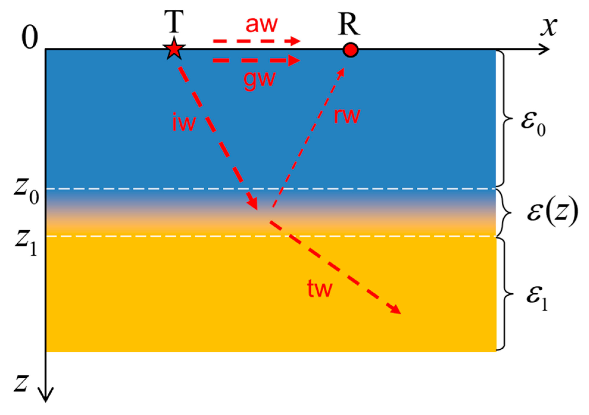
An idealized model of subsurface medium is shown in Figure 4. It consists of a uniform layer with dielectric permittivity (for ) and a half-space with dielectric permittivity , separated by a transition layer where the dielectric permittivity is , . Note that here we call the relative permittivity of the uniform upper layer occupying the region (not the absolute permittivity of a vacuum in SI unit system). The transmitting and receiving antennas, T and R, are placed on the earth surface, at . In the figure, the components of the emitted electromagnetic pulse are shown: aw and gw indicate the “aerial” and “ground” waves, respectively; iw is the incident wave impinging on the transition layer; and rw and tw are the waves reflected and transmitted by the transition layer, respectively.
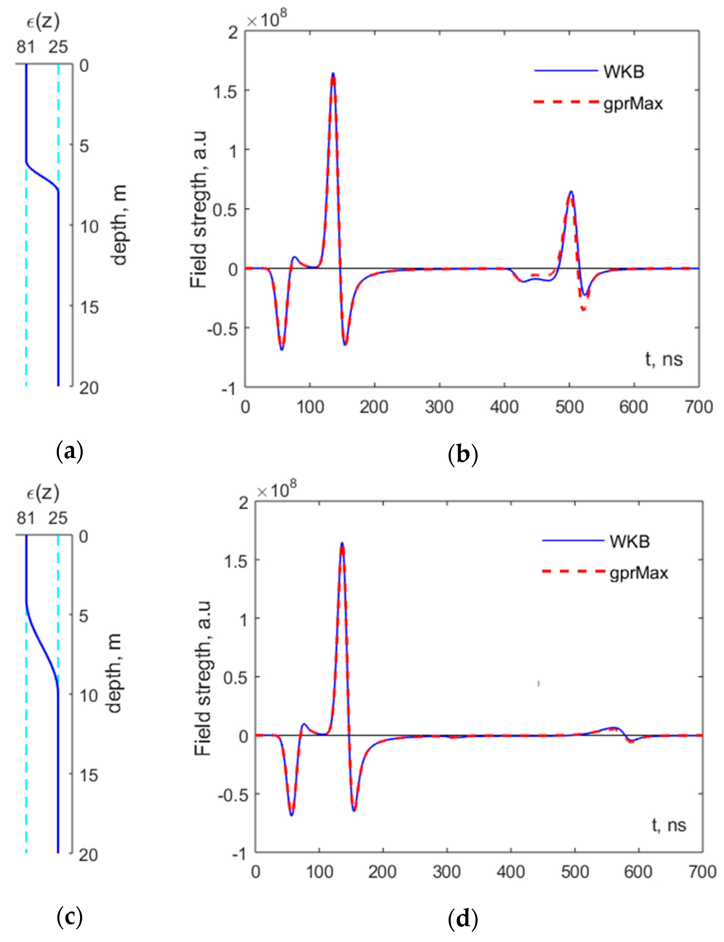
Figure 5a,c model the depth distributions of the dielectric permittivity, corresponding to a gradual transition from pure water () to a hard soil (), in a sweet-water pond with silty bottom. The permittivity profile of the transition layer is given by
corresponds to a transition layer which is located in for Figure 5a, and m for Figure 5c. The distance between the transmitter and receiver antennas is . In Figure 5b,d, synthetic radargrams (A-scans) are presented for the scenarios of Figure 5a,c, respectively. Simulations were performed using both our coupled-WKB method (solid line) and gprMax (dashed line). The first double pulse corresponds to the direct surface wave, propagating along both sides of the ground-air interface. A weak signal with longer delay arises due to the cumulative partial reflection from the non-uniform transition layer.
One can note that, notwithstanding the approximate character of WKB method and the additional errors due to the quasi-vertical approximation, the agreement between the two methods is excellent. It is worth pointing out that our semi-analytical approach, implemented in Matlab R2015 (MathWorks, Inc., Natick, MA, USA), provides a computation time about 100 times shorter than gprMax, version 3.0.0b13 [3,4,5].
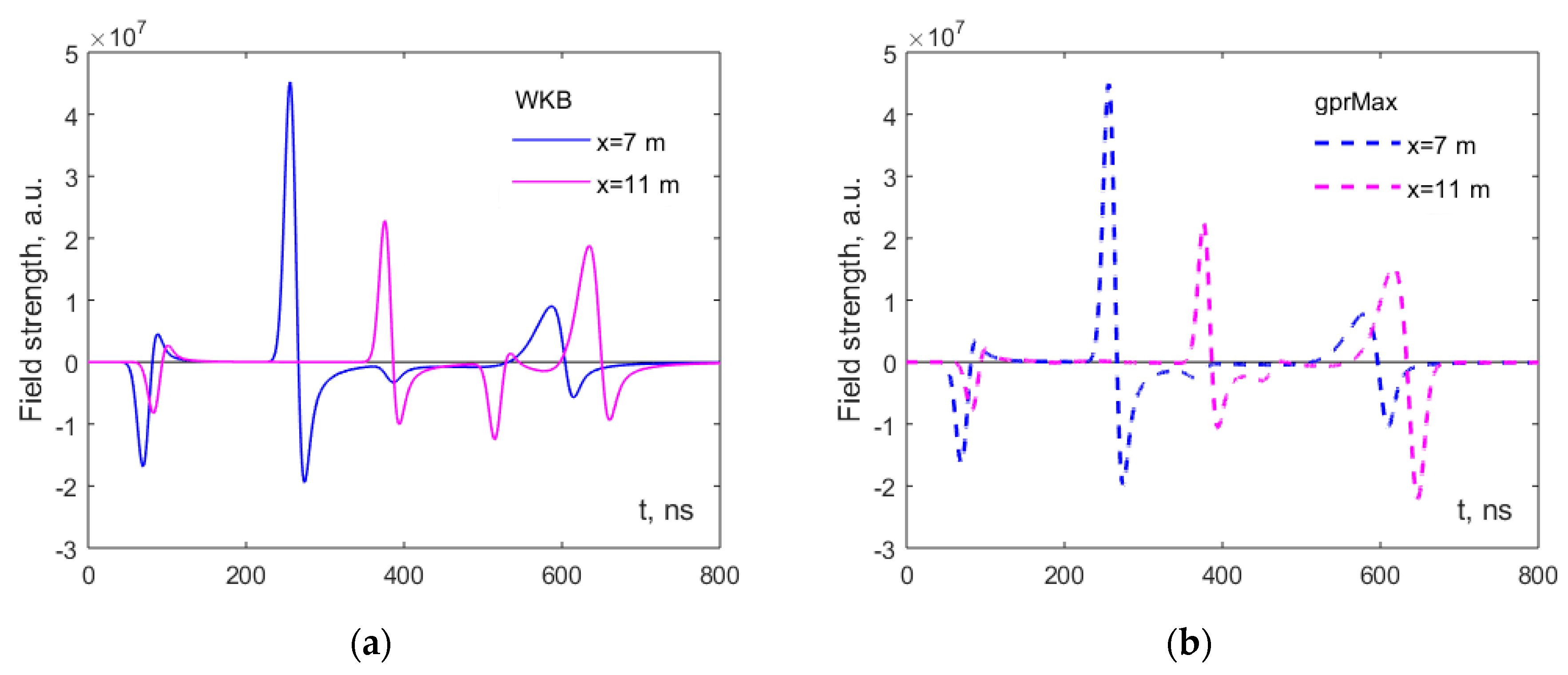
A satisfactory qualitative agreement between FDTD and coupled-WKB results persists even for a larger separation between the antennas, when the propagation path is far from the vertical: see Figure 6a,b, where and . These plots show an interesting effect: a higher amplitude of the reflected signal when the propagation path is longer. This paradoxical behavior, predicted both by the coupled WKB method and by gprMax, can be explained by considering that, when the separation between the antennas is increased, the propagation path follows a direction which is closer to the total-reflection angle.
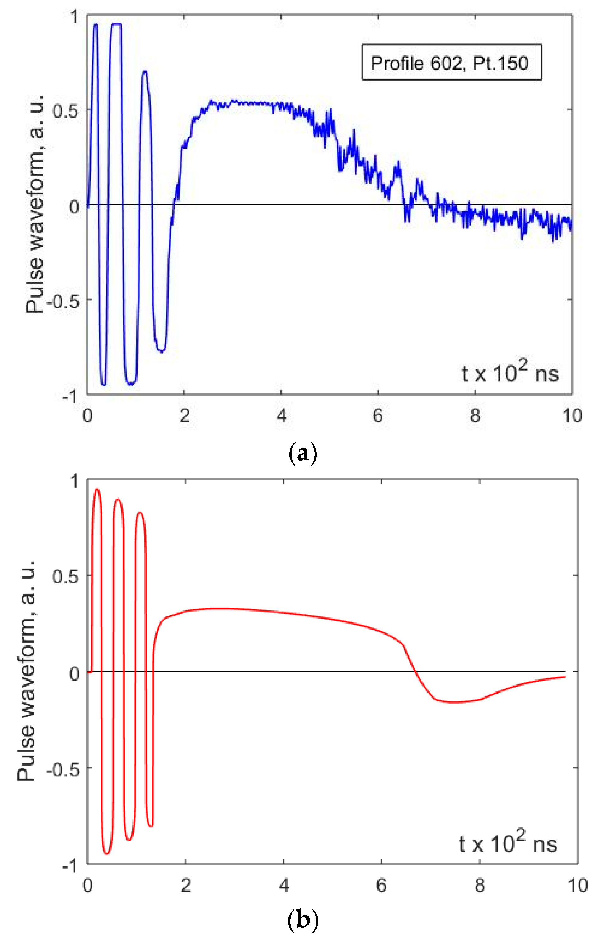
An application of the developed coupled-WKB simulation technique to a real case study is now presented. In particular, the method is applied to the interpretation of GPR radargrams collected on Lake Chebarkul (Chelyabinsk Region, Russia), on the slopes of the southern Urals, during the IZMIRAN field mission in search of a big fragment of the Chelyabinsk meteorite residing in the silty lake floor [31]. The Chelyabinsk meteor reached the Earth on 15 February 2013, and our data were obtained in March 2013 with a low-frequency “Loza-N” GPR [36].
According to divers’ witnesses, the bottom of the lake was covered with a soft silt layer, 2–3 m thick. The experienced “Loza-N” operators assumed that the protracted signals received by the GPR were due to partial reflection from such a loose silt layer. Our numerical simulations with coupled-wave WKB confirm this hypothesis. Indeed, in Figure 7a we present an experimental A-scan showing the aforementioned effect of cumulative partial reflection from a thick layer of bottom sludge; and in Figure 7b we display the numerical results obtained within the framework of our coupled-WKB approximation.
The following values are employed to carry out the simulation. For the pulse radiated by the line source, a damped sinusoid is used, with central frequency . For the ice layer, the relative permittivity is assumed to be , its thickness is 0.8 m. For the transition silt layer, an approximate permittivity profile deduced from the divers’ information and empirically optimized by comparing with the experimental A-scan is , with , , and .
The pulse received by the radar is calculated by convolving the approximate Green function with the chosen current pulse waveform (Duhamel integral [34]), as follows:
As can be appreciated by comparing Figure 7a,b, the simulation qualitatively reproduces the aforementioned effect of protracted reflected pulse; the fast oscillating signal in the left part of the plot corresponds to the direct surface wave and its reflection from the lower ice surface. The similarity of the measured and simulated A-scans confirms the applicability of our approach to real scenarios.
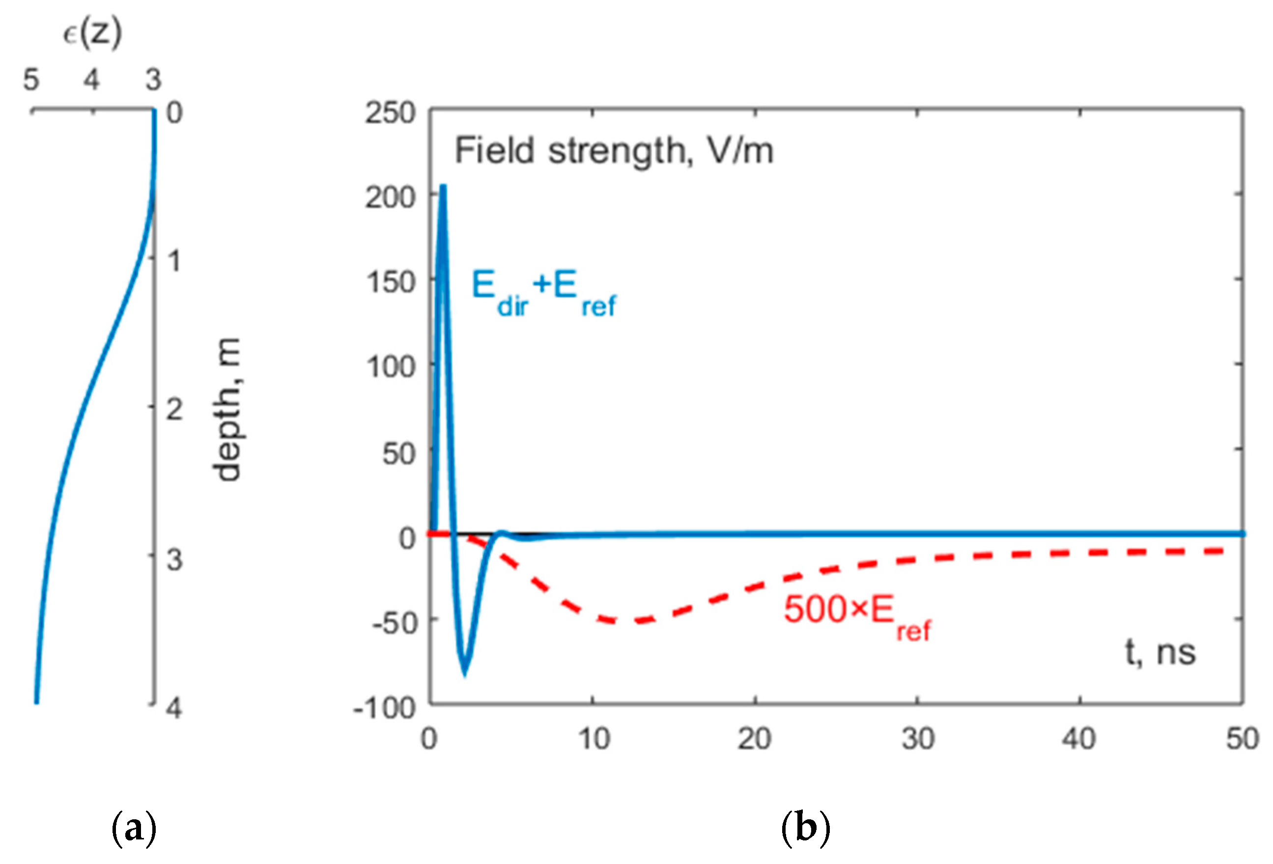
We finally present another possible application of the developed method, namely the interpretation of data that could be obtained by GPR probing the lunar regolith during a planned space mission. It is known that a considerable amount of ice is accumulated in lunar regolith near the poles, which may be used in future space missions. To localize and estimate the available volumes of water, mechanical drilling of lunar regolith [37] can be complemented with GPR probing. The example presented in Figure 8 shows that our semi-analytical approach can be successfully used to model and simulate the electromagnetic propagation of a GPR pulse in the upper regolith layer, characterized by smooth gradients of dielectric permittivity due to the changing ice proportion. For this example, we calculate synthetic A-scans and the reference regolith parameters are taken from the literature [33]. A typical permittivity profile is plotted in Figure 8a and the corresponding A-scan is presented in Figure 8b. The main received signal is a bipolar pulse due to the direct wave propagating from the transmitting to the receiving antenna. The backward reflection is too weak to be seen in the scale of the plot, we therefore multiplied it by and plotted it as a separate curve. Its waveform reveals the cumulative character of the return signal, which is a superposition of partial reflections from the non-uniform transition layer. Despite the weak power level, the backward reflection can be confidently detected with a deep penetration GPR [36]. Valuable information on the smooth subsurface inhomogeneity can be retrieved by comparing simulation results produced with our method and experimental results.
5. Conclusions
We extended the coupled-wave Wentzel-Kramers-Brillouin method (“two-way WKB” approximation) to the case of Ground-Penetrating Radar (GPR) probing of a horizontally-layered dielectric half-space. In particular, we derived an analytical representation of the electromagnetic field excited by a synchronous ultra wideband current pulse in a thin wire stretched along the ground-air interface. A bistatic sounding scheme, commonly used in GPR surveys, was considered. A physical interpretation of the obtained solution was given in terms of geometrical optics and partial reflections from subsurface permittivity gradients. An efficient numerical algorithm was implemented, including an approximate solution of a complex eikonal equation and a high-precision quadrature of the arising singular integrals. Similarities with the coupled parabolic equation method were pointed out.
While our analytical approach is suitable to model the GPR sensing of shallower and deeper layers, the numerical implementation presented in this paper assumes a relatively small separation between the transmitter and the receiver, which allows to shorten the calculation times and makes our method suitable to be embedded into inversion techniques requiring the fast solution of a high number of forward-scattering problems. Specifically, Formulas (32–34) of Section 2.2 yield a general representation of the time-domain coupled-WKB Green function for arbitrary depths and antenna separation. It holds also for the geometric-optical approximation (42) of Section 2.3, valid for short pulses propagating within a narrow strip (“wave film”) behind the GO wave front. Only quasi-vertical approximation discussed in Section 2.4 and implemented in Section 3 requires the assumption of depths exceeding the separation between the transmitter and the receiver. This simplification is valid when modelling monostatic GPR systems (where the same antenna is used for transmitting and receiving signals), as well as bistatic systems if the probed layers are deep enough.
Numerical results of our method were compared with finite-difference time-domain (FDTD) calculations, with very good agreement. Then, two applications to real scenarios were presented. First, our technique was applied to the interpretation of GPR radargrams collected on Lake Chebarkul, in search of a fragment of the Chelyabinsk meteorite. We showed how numerical simulation helps to analyze the protracted return signals originated in smooth transition layers of subsurface dielectric medium. The second example suggests that our method can be used for the estimation of water content in lunar regolith, the upper layer of which contains smooth gradients of permittivity due to gradually increasing fraction of ice.
The good accuracy and numerical efficiency of our semi-analytical computational approach make promising its further development. The approach can be extended to the case of a half-space where the permittivity varies in two directions. Furthermore, we plan to take into account the dissipative and frequency-dispersive behavior of materials by using a complex-valued model of dielectric permittivity in the frequency-domain. The finite length of the antennas and a three-dimensional (3D) gradual variation of the medium parameters will be introduced in a 3D version of the algorithm. We also wish to explore possibilities of hybridization of our approach with FDTD and time-domain integral-equation methods, to capitalize on the strengths of each technique.
Acknowledgments
A considerable part of this work was carried out during two Short-Term Scientific Missions (STSMs) funded by COST (European Cooperation in Science and Technology) Action TU1208 “Civil engineering applications of Ground Penetrating Radar” (www.cost.eu, www.GPRadar.eu). Both missions were kindly hosted by the National Institute of Telecommunications of Poland, in Warsaw. The authors thank COST for funding and supporting the Action TU1208 “Civil engineering applications of Ground Penetrating Radar”. The authors thank the National Institute of Telecommunications of Poland for hosting the STSMs and for paying the article processing charge.
Author Contributions
Alexei Popov and Marian Marciniak developed the theoretical approach to the problem. Igor Prokopovich implemented the method and obtained preliminary numerical results during the first STSM, under the supervision of Marian Marciniak. The analysis was completed by Alexei Popov during the second STSM, in collaboration with Marian Marciniak. Lara Pajewski substantively revised the work carried out during the two STSMs. Then, Igor Prokopovich perfected the numerical implementation and calculated the results presented in this paper, under the supervision of Alexei Popov. All authors contributed to the analysis, interpretation and discussion of results. The text of this paper was written by Lara Pajewski, Alexei Popov and Igor Prokopovich, and was checked and revised by all the authors.
Conflicts of Interest
The authors declare no conflict of interest.
References
- Benedetto, A.; Pajewski, L. (Eds.) Civil Engineering Applications of Ground Penetrating Radar; Book Series: “Springer Transactions in Civil and Environmental Engineering”; Springer: New Delhi, India, 2015; p. 385. ISBN 978-3-319-04813-0. [Google Scholar] [CrossRef]
- Persico, R. Introduction to Ground Penetrating Radar: Inverse Scattering and Data Processing; Wiley-IEEE Press: New York, NY, USA, 2014; p. 392. ISBN 978-1-118-30500-3. [Google Scholar]
- Giannopoulos, A. Modelling ground penetrating radar by GprMax. Constr. Build. Mater. 2005, 19, 755–762. [Google Scholar] [CrossRef]
- Warren, C.; Giannopoulos, A.; Giannakis, I. An advanced GPR modelling framework—The next generation of gprMax. In Proceedings of the 8th International Workshop on Advanced Ground Penetrating Radar (IWAGPR 2015), Florence, Italy, 7–10 July 2015; pp. 1–4. [Google Scholar] [CrossRef]
- Warren, C.; Giannopoulos, A. Experimental and Modeled Performance of a Ground Penetrating Radar Antenna in Lossy Dielectrics. IEEE J. Sel. Top. Appl. Earth Obs. Remote Sens. 2016, 9, 29–36. [Google Scholar] [CrossRef]
- Frezza, F.; Mangini, F.; Pajewski, L.; Schettini, G.; Tedeschi, N. Spectral domain method for the electromagnetic scattering by a buried sphere. J. Opt. Soc. Am. A 2013, 30, 783–790. [Google Scholar] [CrossRef] [PubMed]
- Frezza, F.; Pajewski, L.; Ponti, C.; Schettini, G.; Tedeschi, N. Cylindrical-Wave Approach for Electromagnetic Scattering by Subsurface Metallic Targets in a Lossy Medium. J. Appl. Geophys. 2013, 97, 55–59. [Google Scholar] [CrossRef]
- Frezza, F.; Pajewski, L.; Ponti, C.; Schettini, G.; Tedeschi, N. Electromagnetic Scattering by a Metallic Cylinder Buried in a Lossy Medium with the Cylindrical-Wave Approach. IEEE Geosci. Remote Sens. Lett. 2013, 10, 179–183. [Google Scholar] [CrossRef]
- Bourlier, C.; Le Bastard, C.; Pinel, N. Full wave PILE method for the electromagnetic scattering from random rough layers. In Proceedings of the 15th International Conference on Ground Penetrating Radar (GPR 2014), Brussels, Belgium, 30 June–4 July 2014; pp. 545–551. [Google Scholar] [CrossRef]
- Poljak, D.; Dorić, V. Transmitted field in the lossy ground from ground penetrating radar (GPR) dipole antenna. WIT Trans. Model. Simul. 2015, 59, 3–11. [Google Scholar] [CrossRef]
- Poljak, D.; Dorić, V.; Birkić, M.; El Khamlichi Drissi, K.; Lallechere, S.; Pajewski, L. A simple analysis of dipole antenna radiation above a multilayered medium. In Proceedings of the 9th International Workshop on Advanced Ground Penetrating Radar (IWAGPR 2017), Edinburgh, UK, 28–30 June 2017; pp. 1–6. [Google Scholar] [CrossRef]
- Winton, S.C.; Kosmas, P.; Rappaport, C.M. FDTD simulation of TE and TM plane waves at nonzero incidence in arbitrary layered media. IEEE Trans. Antennas Propag. 2005, 53, 1721–1728. [Google Scholar] [CrossRef]
- Diamant, R.; Fernandez-Guasti, M. Light propagation in 1D inhomogeneous deterministic media: The effect of discontinuities. J. Opt. A Pure Appl. Opt. 2009, 11, 045712. [Google Scholar] [CrossRef]
- Zeng, Q.; Delisle, G.Y. Transient analysis of electromagnetic wave reflection from a stratified medium. In Proceedings of the 2010 Asia-Pacific International Symposium on Electromagnetic Compatibility, Beijing, China, 12–16 April 2010; pp. 881–884. [Google Scholar] [CrossRef]
- Kaganovsky, Y.; Heyman, E. Pulsed beam propagation in plane stratified media: Asymptotically exact solutions. In Proceedings of the 2010 URSI International Symposium on Electromagnetic Theory, Berlin, Germany, 16–19 August 2010; pp. 829–832. [Google Scholar] [CrossRef]
- Diamanti, N.; Annan, A.P.; Redman, J.D. Impact of Gradational Electrical Properties on GPR Detection of Interfaces. In Proceedings of the 15th International Conference on Ground Penetrating Radar (GPR 2014), Brussels, Belgium, 30 June–4 July 2014; pp. 529–534. [Google Scholar] [CrossRef]
- Connor, K.M.; Dowding, C.H. GeoMeasurements by Pulsing TDR Cables and Probes; CRC Press: Boca Raton, FL, USA, 1999; p. 424. ISBN 9780849305863. [Google Scholar]
- Schlaeger, S. Inversion of TDR Measurements to Reconstruct Spatially Distributed Geophysical Ground Parameter. Ph.D. Thesis, University of Karlsruhe, Karlsruhe, Germany, 2002. [Google Scholar]
- Epstein, P.S. Reflection of waves in an inhomogeneous absorbing medium. Proc. Natl. Acad. Sci. USA 1930, 16, 627–637. [Google Scholar] [CrossRef] [PubMed]
- Weiland, T. A discretization model for the solution of Maxwell’s equations for six-component fields. Archiv Elektronik Uebertragungstechnik 1977, 31, 116–120. [Google Scholar]
- Miller, E.K.; Poggio, A.J.; Burke, G.J. An integro-differential equation technique for the time-domain analysis of thin wire structures. I. the numerical method. J. Comput. Phys. 1973, 12, 24–48. [Google Scholar] [CrossRef]
- Krueger, R.J.; Ochs, R.L., Jr. A Green’s function approach to the determination of internal fields. Appl. Math. Sci. 1989, 11, 525–543. [Google Scholar] [CrossRef]
- Lambot, S.; Slob, E.; Vereecken, H. Fast evaluation of zero-offset Green’s function for layered media with application to ground-penetrating radar. Geophys. Res. Lett. 2007, 34, L21405. [Google Scholar] [CrossRef]
- Larruquert, J.I. Reflectance optimization of inhomogeneous coatings with continuous variation of the complex refractive index. J. Opt. Soc. Am. A 2006, 23, 99–107. [Google Scholar] [CrossRef]
- Grafstrom, S. Reflectivity of a stratified half-space: The limit of weak inhomogeneity and anisotropy. J. Opt. A Pure Appl. Opt. 2006, 8, 134–141. [Google Scholar] [CrossRef]
- Landau, L.D.; Lifshits, E.M. Quantum Mechanics: Non-Relativistic Theory; Butterworth-Heinemann: Oxford, UK, 1977; p. 677. ISBN 0750635398. [Google Scholar]
- Brekhovskikh, L.M. Waves in Layered Media, 2nd ed.; Academic Press: New York, NY, USA, 1980; 520p, ISBN 9780323161626. [Google Scholar]
- Bremmer, H. Propagation of Electromagnetic Waves. In Handbuch der Physik/Encyclopedia of Physics; Flugge, S., Ed.; Springer: Berlin/Goettingen/Heidelberg, Germany, 1958; Volume 4/16, pp. 423–639. [Google Scholar]
- Jones, A.R. Light scattering for particle characterization. Prog. Energy Comb. Sci. 1999, 25, 1–53. [Google Scholar] [CrossRef]
- Vinogradov, V.A.; Kopeikin, V.V.; Popov, A.V. An approximate solution of 1D inverse problem. In Proceedings of the 10th International Conference on Ground Penetrating Radar (GPR 2004), Delft, The Netherlands, 21–24 June 2004; pp. 95–98. [Google Scholar]
- Kopeikin, V.V.; Kuznetsov, V.D.; Morozov, P.A.; Popov, A.V.; Berkut, A.I.; Merkulov, S.V.; Alexeev, V.A. Ground Penetrating Radar Investigation of the Supposed Fall Site of a Fragment of the Chelabinsk Meteorite in Lake Chebarkul. Geochem. Int. 2013, 51, 636–642. [Google Scholar] [CrossRef]
- Buzin, V.; Edemsky, D.; Gudoshnikov, S.; Kopeikin, V.; Morozov, P.; Popov, A.; Prokopovich, I.; Skomarovsky, V.; Melnik, N.; Berkut, A.; et al. Search for Chelyabinsk Meteorite Fragments in Chebarkul Lake Bottom (GPR and Magnetic Data). J. Telecommun. Inf. Technol. 2017, 2017, 69–78. [Google Scholar] [CrossRef]
- Olhoeft, G.R.; Strangway, D.W. Dielectric Properties of the First 100 Meters of the Moon. Earth Planet. Sci. Lett. 1975, 24, 394–404. [Google Scholar] [CrossRef]
- Fritz, J. Partial Differential Equations, 4th ed.; Springer: New York, NY, USA, 1982; p. 672. ISBN 978-0-387-90609-6. [Google Scholar]
- Claerbout, J.F. Fundamentals of Geophysical Data Processing; Pennwell Books: Tulsa, OK, USA, 1985; 274p, ISBN 0865423059. [Google Scholar]
- Berkut, A.I.; Edemsky, D.E.; Kopeikin, V.V.; Morozov, P.A.; Prokopovich, I.V.; Popov, A.V. Deep penetration subsurface radar: Hardware, results, interpretation. In Proceedings of the 9th International Workshop on Advanced Ground Penetrating Radar (IWAGPR 2017), Edinburgh, UK, 7–10 July 2017; pp. 1–6. [Google Scholar] [CrossRef]
- Matveev, Y.I.; Kostenko, V.I. Problems of Moving Ultrasound Penetrative Devices in a Dispersion Medium during Drilling of the Moon’s Regolith. Acoust. Phys. 2016, 62, 633–641. [Google Scholar] [CrossRef]
Figure 1.
Color map of the exponential in Equation (29), with the steepest descent path, and poles of the integrand.
Figure 1.
Color map of the exponential in Equation (29), with the steepest descent path, and poles of the integrand.
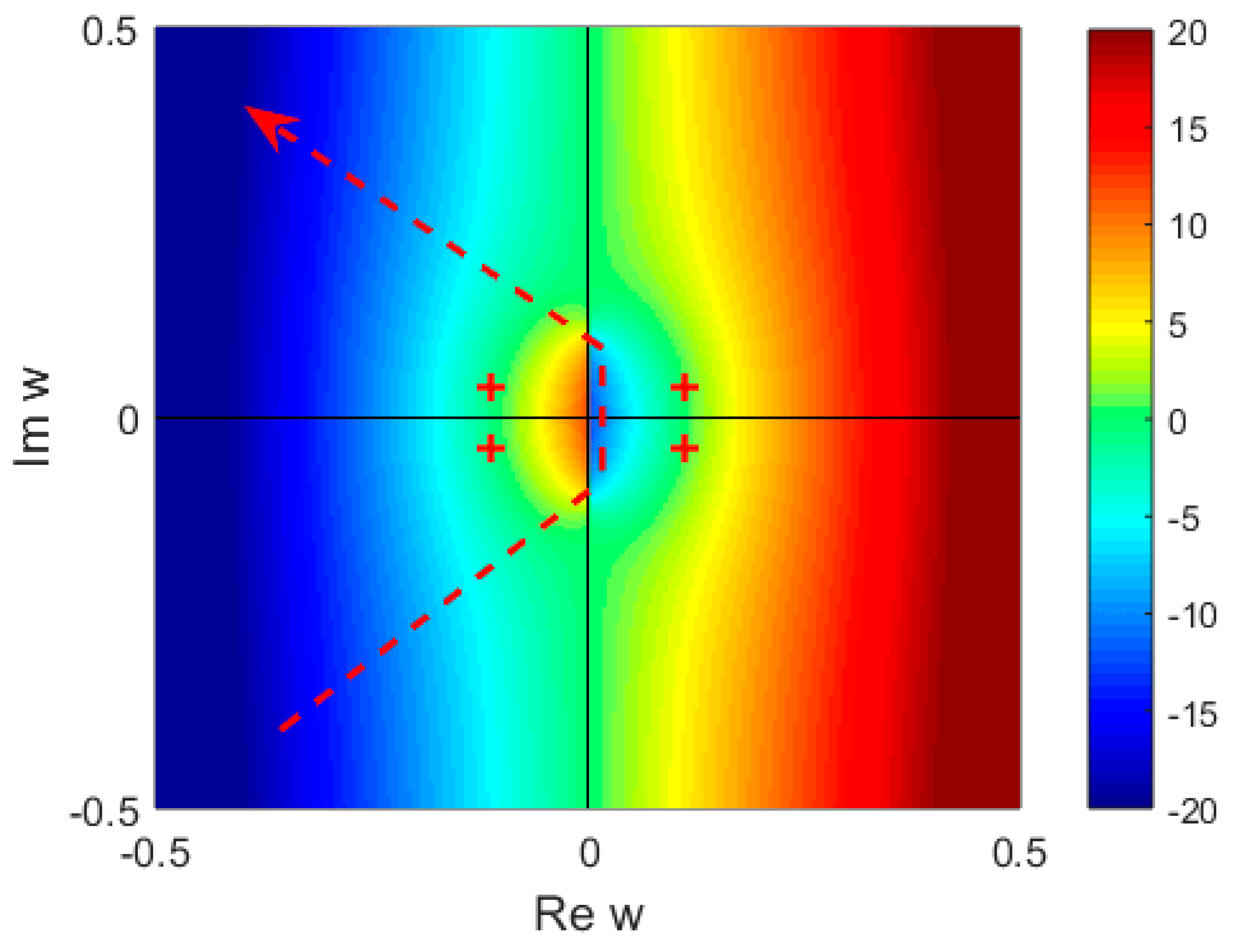
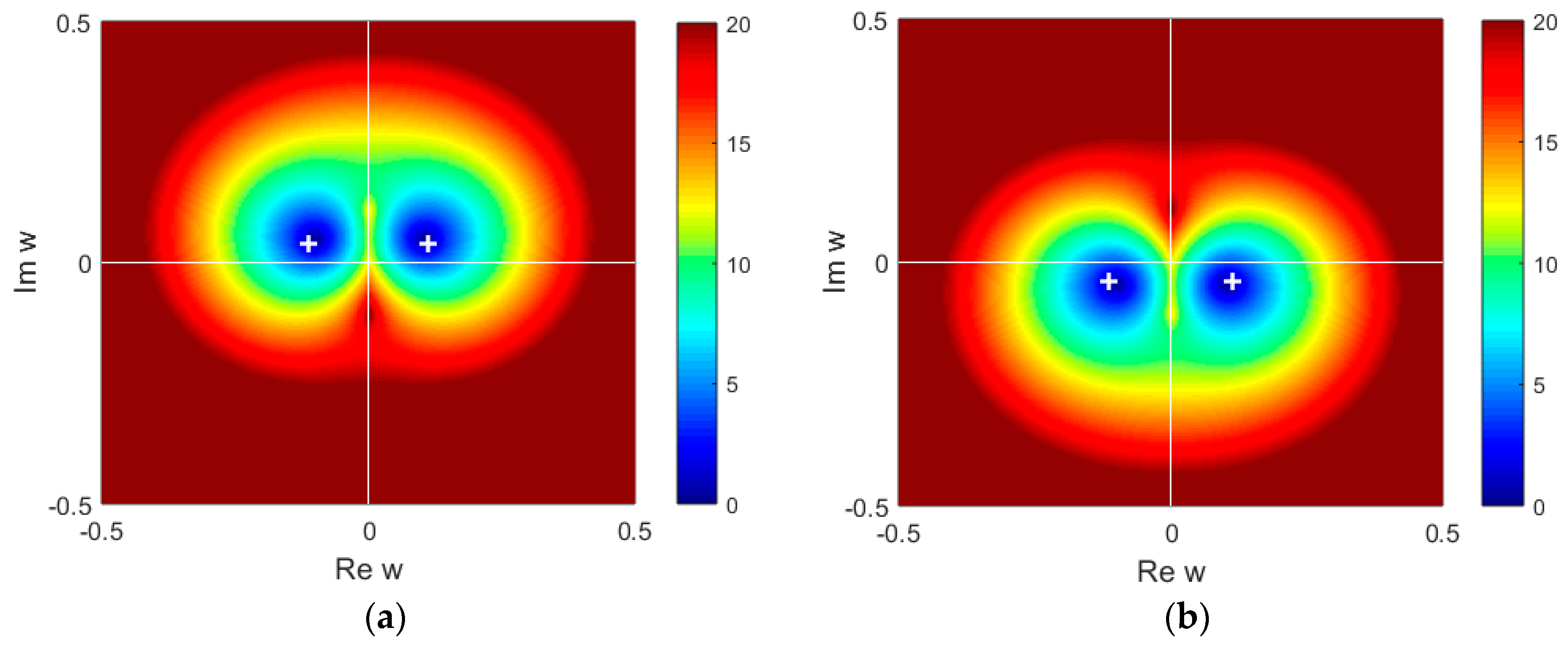
Figure 2.
Roots of the functional Equation (35), corresponding to the: upper (a); and lower (b) signs in the right-hand side, for x = 4 m, , , m, m.
Figure 2.
Roots of the functional Equation (35), corresponding to the: upper (a); and lower (b) signs in the right-hand side, for x = 4 m, , , m, m.

Figure 3.
Partial reflection of the probing pulse due to the permittivity gradient. T and R are the transmitter and receiver positions, respectively. The red dashed line represents the GO path, while the white dashed line refers to an effective level of partial reflection.
Figure 3.
Partial reflection of the probing pulse due to the permittivity gradient. T and R are the transmitter and receiver positions, respectively. The red dashed line represents the GO path, while the white dashed line refers to an effective level of partial reflection.
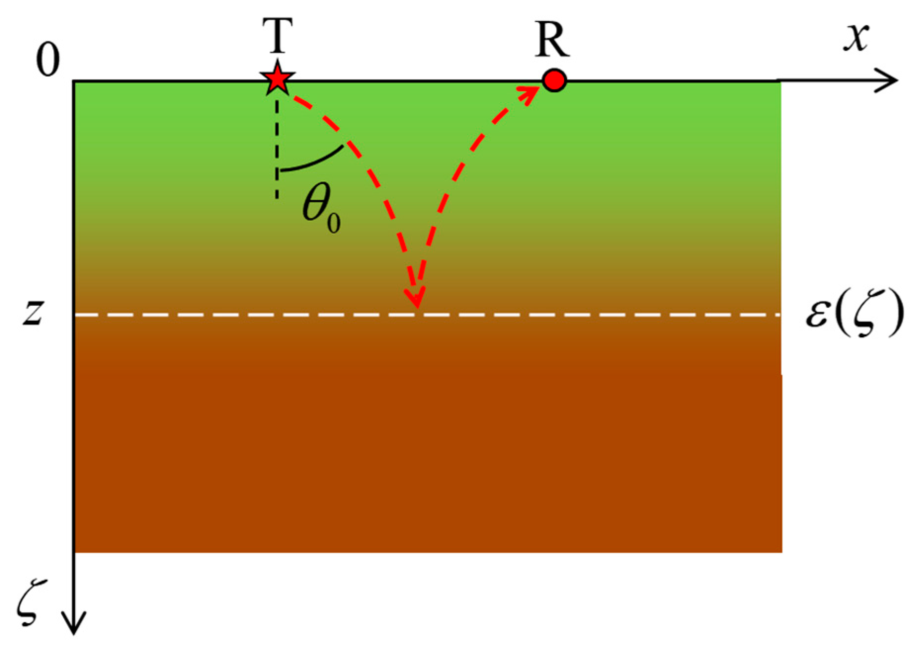
Figure 4.
Geometry of the simulated scenario and schematic representation of the radar signal components.
Figure 4.
Geometry of the simulated scenario and schematic representation of the radar signal components.

Figure 5.
Two vertical profiles of the dielectric permittivity are shown in (a,c). The corresponding simulated A-scans (coupled WKB: solid line, gprMax: dashed line) are shown in (b,d), respectively.
Figure 5.
Two vertical profiles of the dielectric permittivity are shown in (a,c). The corresponding simulated A-scans (coupled WKB: solid line, gprMax: dashed line) are shown in (b,d), respectively.

Figure 6.
A-scans simulated with: (a) our coupled WKB method (solid lines); and (b) gprMax (dashed lines), for larger distances between transmitter and receiver.
Figure 6.
A-scans simulated with: (a) our coupled WKB method (solid lines); and (b) gprMax (dashed lines), for larger distances between transmitter and receiver.

Figure 7.
(a) Experimental A-scan with a protracted reflected pulse, recorded on the iced surface of Lake Chebarkul by GPR probing the silty bottom; and (b) synthetic A-scan calculated using our coupled-wave WKB approach.
Figure 7.
(a) Experimental A-scan with a protracted reflected pulse, recorded on the iced surface of Lake Chebarkul by GPR probing the silty bottom; and (b) synthetic A-scan calculated using our coupled-wave WKB approach.

Figure 8.
GPR probing of lunar regolith (numerical simulation): (a) reference permittivity profile; and (b) received pulse, including both the direct wave and weak subsurface reflection (blue), and magnified subsurface reflection (red).
Figure 8.
GPR probing of lunar regolith (numerical simulation): (a) reference permittivity profile; and (b) received pulse, including both the direct wave and weak subsurface reflection (blue), and magnified subsurface reflection (red).

© 2017 by the authors. Licensee MDPI, Basel, Switzerland. This article is an open access article distributed under the terms and conditions of the Creative Commons Attribution (CC BY) license (http://creativecommons.org/licenses/by/4.0/).
Share and Cite
MDPI and ACS Style
Prokopovich, I.; Popov, A.; Pajewski, L.; Marciniak, M. Application of Coupled-Wave Wentzel-Kramers-Brillouin Approximation to Ground Penetrating Radar. Remote Sens. 2018, 10, 22. https://doi.org/10.3390/rs10010022
AMA Style
Prokopovich I, Popov A, Pajewski L, Marciniak M. Application of Coupled-Wave Wentzel-Kramers-Brillouin Approximation to Ground Penetrating Radar. Remote Sensing. 2018; 10(1):22. https://doi.org/10.3390/rs10010022
Chicago/Turabian StyleProkopovich, Igor, Alexei Popov, Lara Pajewski, and Marian Marciniak. 2018. "Application of Coupled-Wave Wentzel-Kramers-Brillouin Approximation to Ground Penetrating Radar" Remote Sensing 10, no. 1: 22. https://doi.org/10.3390/rs10010022
Note that from the first issue of 2016, this journal uses article numbers instead of page numbers. See further details here.