Unsupervised Clustering Method for Complexity Reduction of Terrestrial Lidar Data in Marshes


1
College of Science and Engineering, Texas A&M University-Corpus Christi, Corpus Christi, TX 78412, USA
2
School of Engineering and Computing Sciences, Conrad Blucher Institute for Surveying and Science, Texas A&M University-Corpus Christi, Corpus Christi, TX 78412, USA
3
Harte Research Institute, Texas A&M University-Corpus Christi, Corpus Christi, TX 78412, USA
*
Author to whom correspondence should be addressed.
Remote Sens. 2018, 10(1), 133; https://doi.org/10.3390/rs10010133
Submission received: 4 November 2017
/
Revised: 11 December 2017
/
Accepted: 28 December 2017
/
Published: 18 January 2018
(This article belongs to the Special Issue 3D Modelling from Point Clouds: Algorithms and Methods)
Abstract
:Accurate characterization of marsh elevation and landcover evolution is important for coastal management and conservation. This research proposes a novel unsupervised clustering method specifically developed for segmenting dense terrestrial laser scanning (TLS) data in coastal marsh environments. The framework implements unsupervised clustering with the well-known K-means algorithm by applying an optimization to determine the “k” clusters. The fundamental idea behind this novel framework is the application of multi-scale voxel representation of 3D space to create a set of features that characterizes the local complexity and geometry of the terrain. A combination of point- and voxel-generated features are utilized to segment 3D point clouds into homogenous groups in order to study surface changes and vegetation cover. Results suggest that the combination of point and voxel features represent the dataset well. The developed method compresses millions of 3D points representing the complex marsh environment into eight distinct clusters representing different landcover: tidal flat, mangrove, low marsh to high marsh, upland, and power lines. A quantitative assessment of the automated delineation of the tidal flat areas shows acceptable results considering the proposed method is unsupervised with no training data. Clustering results based on K-means are also compared to results based on the Self Organizing Map (SOM) clustering algorithm. Results demonstrate that the developed multi-scale voxelization approach and representative feature set are transferrable to other clustering algorithms, thereby providing an unsupervised framework for intelligent scene segmentation of TLS point cloud data in marshes.
1. Introduction
Marshes have long been recognized as integral systems containing high biological productivity and diversity within the global ecosystem [1,2,3,4]. Positioned at the interface between aquatic and upland environments, they provide habitat for both aquatic and terrestrial organisms and perform critical nutrient cycling functions including waste regulation and water purification [1,2,3]. They also provide upland areas with a buffer against coastal hazards such as storms and hurricanes and are capable of mitigating shoreline erosion and attenuating floodwaters [5]. However, marshes are intertidal areas often located at low elevation with very little topographic relief. Even a small topographic change can cause major impacts on wetland ecosystems such as water flow, sediment deposition, and the amplitude and frequency of inundation [6,7,8]. Elevation changes of less than a few cm have a significant effect on plant distribution and productivity [6,7,8]. Hence, sea level rise (slr) associated with climate change and land subsidence pose major challenges for the management and conservation of marsh environments. The rate of slr has accelerated from approximately 1.7 + 0.3 mm/year during the 20th century [9] to about 3.4 +/−0.4 mm/year at present [10]. In many coastal areas such as the Northwest Gulf of Mexico, vertical land motion contributes a substantial component to the overall relative sea level rise (rslr). Due to their low elevations above mean sea level, the frequency of inundation of marshes associated with rslr will increase at a much higher rate than inundations associated to storm events [11]. Sediment accretion is a natural response that contributes to changes in elevation of a marsh surface relative to sea level. For a marsh to sustain its ecosystem function, its accretion rate must be at least equal to the pace of the rslr at its location as the vertical elevation of the marsh relative to mean sea level is critical for its productivity and stability [12]. Therefore, it is important to accurately characterize salt marsh surface elevation, landcover, and their changes to be able to predict whether salt marsh wetlands and the ecosystem function they support can withstand an accelerated rise in sea level.
Terrestrial Laser Scanning (TLS), also referred to as terrestrial light detection and ranging (lidar), uses a lidar scanner mounted on a tripod to 3D image a scene. Lidar is an active remote sensing technology that measures the distance between the sensor and an object, most commonly by recording the laser pulse time-of-flight. This is done by precisely measuring the elapsed time between the emission of a laser pulse and the arrival of the reflection of that pulse to the sensor’s receiver [13]. TLS is able to record a large amount of topographic information with a sub-cm sampling density over an extended area in a relatively short period. Over the past decade, TLS technology has been widely applied to collect data at local spatial scales with fine point spacing [14,15,16]. The use of TLS is now well established in geology and landscape dynamics [17,18,19,20]. More recently, its potential in fluvial geomorphology [21,22], floodplain mapping [16], soil science [23], and wetland mapping [24,25,26,27] have begun to be explored. However, within the coastal marsh environment, the ability of TLS systems to resolve centimeter-level elevation differences between the vegetation and the bare earth surface is limited [28,29,30].
Extraction of ground and vegetation (landcover) information from TLS point cloud data of a marsh environment is a difficult task because of the complexity of the laser pulse interaction with the variety of vegetative structure, underlying topography including moist and dry ground, water, and other structures. The resultant scans provide a very complex 3D scene representation consisting of millions or hundreds of millions of points that cannot be individually segmented into homogeneous features (e.g., bare ground) without the use of intelligent data segmentation algorithms. The identification of points being from the ground, vegetation or anthropogenic structures requires filtering the data into like-groups or classes. To do so, methods must be developed and implemented to identify structure in the data prior to creation of a TLS end-product (e.g., digital elevation model of the tidal flat area). A voxel representation of 3D space provides a quantitative method to assess neighborhood properties in the TLS point cloud and coupled with individual point characteristics provides inputs for conducting pattern recognition. Inspired by the earlier octree-based method of [31], this research introduces a new voxel-based unsupervised method specifically developed for segmenting TLS point cloud data in coastal marsh environments. One major difference between this study’s approach and [31] is the criterion for the merging procedure. [31] merged voxelized point groups directly to each other based on proximity and coplanarity; points of neighboring subspaces were recursively merged if they passed a coplanar test. Coplanar point groups were then merged into “co-surface” point groups based on plane connection and intersection criteria. In contrast, this research merges points based on the similarity of various features computed from multi-scale voxelization of the point cloud data and from individual point features using unsupervised machine learning (data clustering). These features are targeted to help describe differences in the scan characteristics due to varying properties of the imaged landscape. In this way, the algorithm describes the complexity of the imaged scene in an automated framework. This approach allows one to search for patterns in the point cloud data including identifying ground and vegetation points as well as other unforeseen patterns. This method is referred to as automated reduction of TLS data complexity for marsh scene compression as the method will breakup very complex and dense point cloud data into homogeneous groups (clusters) of points representing different terrain and landcover features.
2. Study Areas and Dataset
2.1. Study Site
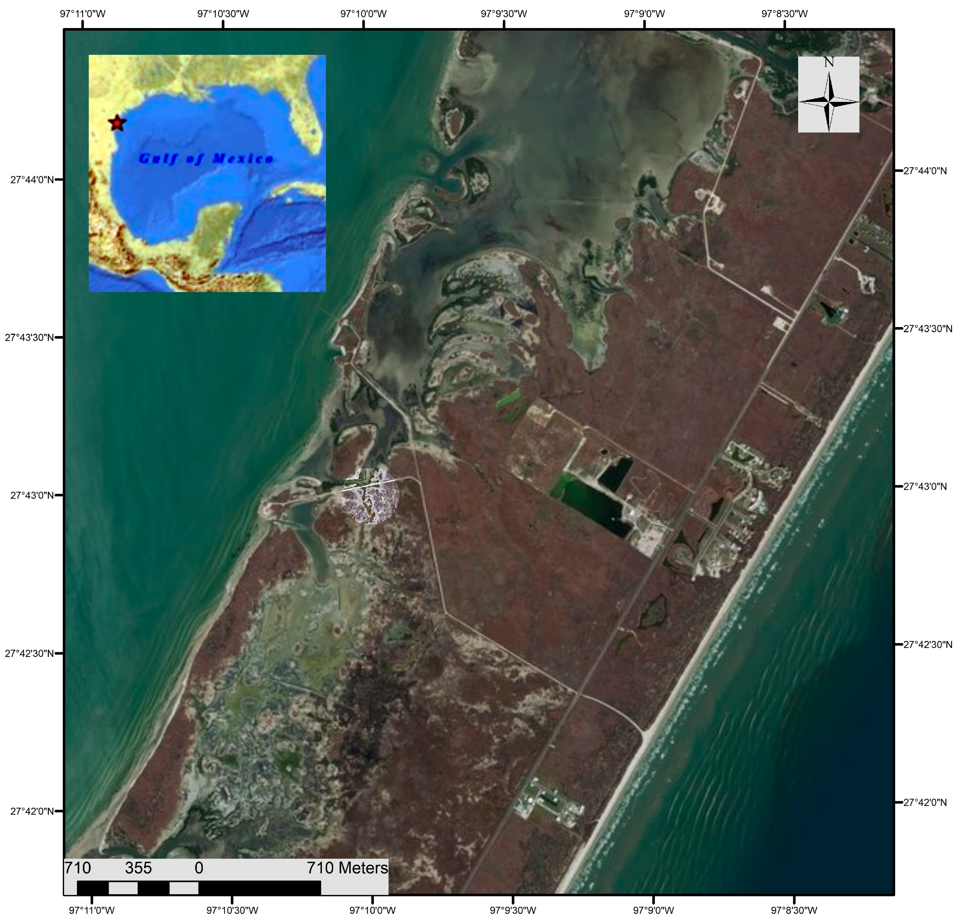
The study site is a marsh located on a barrier island along the southern portion of the Texas Gulf Coast, USA, bounded by Corpus Christi Bay, the Laguna Madre, and the Gulf of Mexico called the Mustang Island Wetland Observatory (Figure 1 and Figure 2). The study area is located on the bay side of Mustang Island and has a nominal 0.10 m tidal range. It is characterized as a microtidal dominated coast subject to diurnal tides [32]. The width of the barrier island in this region is approximately 2.2 km. Progressing from the Gulf shoreline inland to the Corpus Christi Bay shoreline, upland environment in the region ranges in elevation from approximately 0.52 to 5.49 m (NAVD88); high marsh environment ranges in elevation from 0.2 to 0.8 m; low marsh environment ranges in elevation from −0.1 to 0.3 m; tidal flat environment ranges in elevation from −0.05 to 0.5 m [32]. These elevation ranges overlap because different geo-environments can occur at the same elevation for different locations.
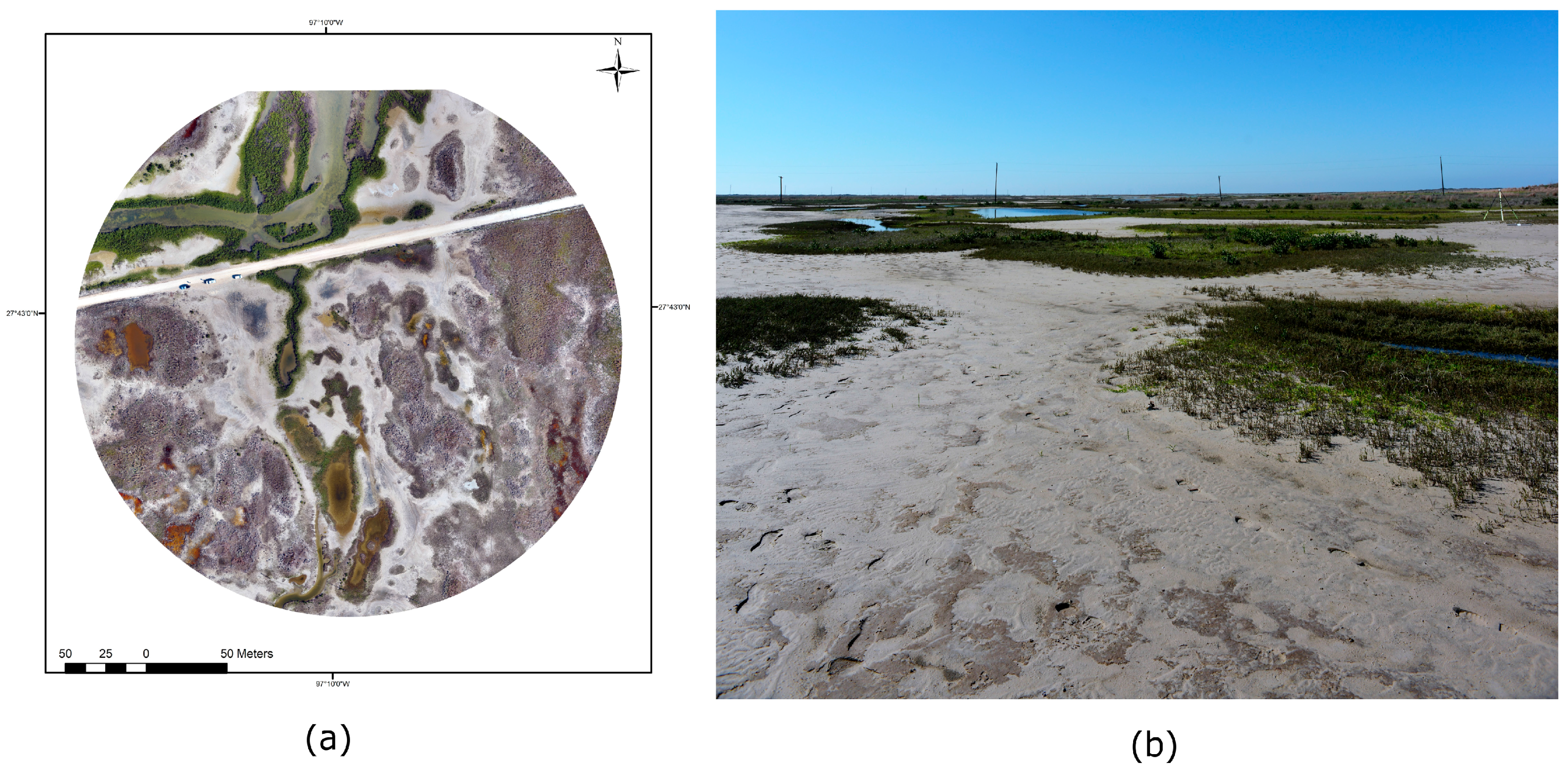
The TLS survey area consists of a transect from upland to high marsh to low marsh, then tidal flat. The average elevation is highest for upland areas and lowest for low tidal flat area. The dominant environment of this study area is upland. The dominant vegetation species are Zchizachyrium littorale (coastal bluestem) and Spartina patens (gulf cordgrass) commonly found growing in mats. The second most prevalent environment of this study area is tidal flat (Figure 2), which are banks of exposed sediment regularly inundated. Tidal flat surfaces slope gently in elevation from mean high tide water level down toward mean spring tide low water level. High tidal flats are typically only partly submerged at high tide, whereas low tidal flats are located at lower elevation and regularly inundated at high tide. Low, regularly flooded tidal/algal flats are significantly less abundant than high flats in this area. These local tidal flats are designated as wind-tidal flats because flooding occurs mainly due to wind-driven tides [9]. Blue-green algae flourish in low tidal flats after long periods of inundation. In some of the study’s tidal flat area, salt marsh vegetation such as M. litoralis (shore medick), Batis maritima (pickle weed), and Salicornia spp. (glasswort) can be found sparingly. Low marsh areas are very high in biologic productivity. More frequently inundated areas near tidal creeks are dominated by Avicennia germinans (black mangrove) with Batis maritima (pickle weed) following. High marsh environment is the least abundant in the study area. It varies in elevation well above the mean high tide, therefore it is rarely inundated. Within the high marsh range, Monanthochloe litoralis (shoregrass) and Salicornia spp. (glasswort) are the dominant species [32].
2.2. Dataset
The Conrad Blucher Institute at Texas A&M University-Corpus Christi conducted a TLS survey of the Mustang Island Wetland Observatory on 14 March 2017 using a VZ-400 scanner manufactured by Riegl in Horn, Austria. The TLS survey was conducted during a spring low tide to minimize the area of water cover on the marsh surface. The 1550 nm near-infrared laser pulse used by this system is heavily absorbed by water or scattered (due to specular reflectance) [33] and hence information cannot be reliably captured from inundated areas. Furthermore, the scanner utilizes online waveform processing to enable multi-return echo detection with up to 10+ echoes per an emitted laser pulse, although such a high number of returns is not expected in a marsh environment. Specifications of the TLS can be found in Table 1.
The TLS was mounted on a leveling tripod two meters above ground level, and a single scan was acquired targeting an approximately 16-hectare area at the study site. The scan was acquired at a full 360° horizontal field of view using the long distance ranging mode (600 m average range dependent on surface albedo). The horizontal and vertical stepping angle was set to 20 millidegrees, which resulted in an average point separation of 3.4 cm at 100 m radial distance from the scanner. Four reflector targets (10 cm cylinders) were spread throughout the scan scene and were subsequently used to georeference the point cloud. All targets were geodetically surveyed with real-time kinematic (RTK) global navigation satellite system (GNSS) positioning using an Altus APS-3 GNSS receiver (Altus Positioning Systems, Torrance, CA, USA). Differential corrections were provided by the Western Data Systems Trimble virtual reference station (VRS) network that offers centimeter-accuracy coordinates. The resultant point cloud consisted of 37,672,870 points with a mean density of 282 points/m2.
For the study presented in this paper, the acquired TLS point cloud data were first clipped at a radial distance of 170 m away from the scanner to focus in on areas of higher point density and less scan occlusion from vegetation (Figure 2a shows this area). Due to the radially decreasing point density inherent with a single TLS scan, an octree filter was applied to better regularize the point spacing near the scanner in high density areas and reduce point density to save computational time [34]. The point clouds were mapped into voxels, and then the centroid of all points within each voxel were used to extract a point per a voxel. The voxel size was set to 2 cm × 2 cm × 1 cm to maintain high spatial detail in the horizontal and vertical component without over redundancy of information [35]. After this process, the number of points for this study’s point cloud was 9,572,446 with a mean density of 186 points/m2. It is important to mention that this voxelization step was only applied to filter the point density prior to clustering. It is not related to the multi-scale voxelization procedure for feature extraction described in Section 3.2 below.
A small-unmanned aircraft system (UAS) survey was also conducted at the same time as the TLS survey using a DJI Phantom 4 UAV equipped with a 12.4 MP RGB camera. Accurate georeferencing of the acquired imagery is critical for comparison to the TLS point cloud data. Without proper ground control, the raw positional accuracy of the acquired imagery stemming solely from geotagging by the UAS platform’s onboard single-channel, non-differential GPS is roughly 1 to 5 m. Five aerial ground control targets (1.2 m × 0.8 m planar target with black and white bulls eye pattern) were placed at four corners and midpoint of the survey area. The target positions (x, y, z) were surveyed using the same RTK GNSS receiver and differential correction method applied to survey the TLS cylindrical targets as described above. This enabled horizontal positioning accuracy within 1 to 5 cm, which ensured consistent registration with the TLS point cloud data. A high resolution orthomosaic (1.5 cm ground sample distance) was generated from the overlapping image sequence using structure-from-motion photogrammetry. The resultant orthomosaic was used to aid in ground truthing and validate the clustering results (see Figure 2a).
3. Method
3.1. Overview
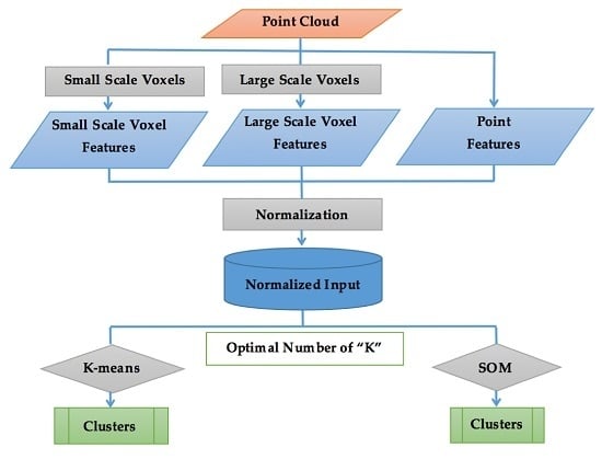
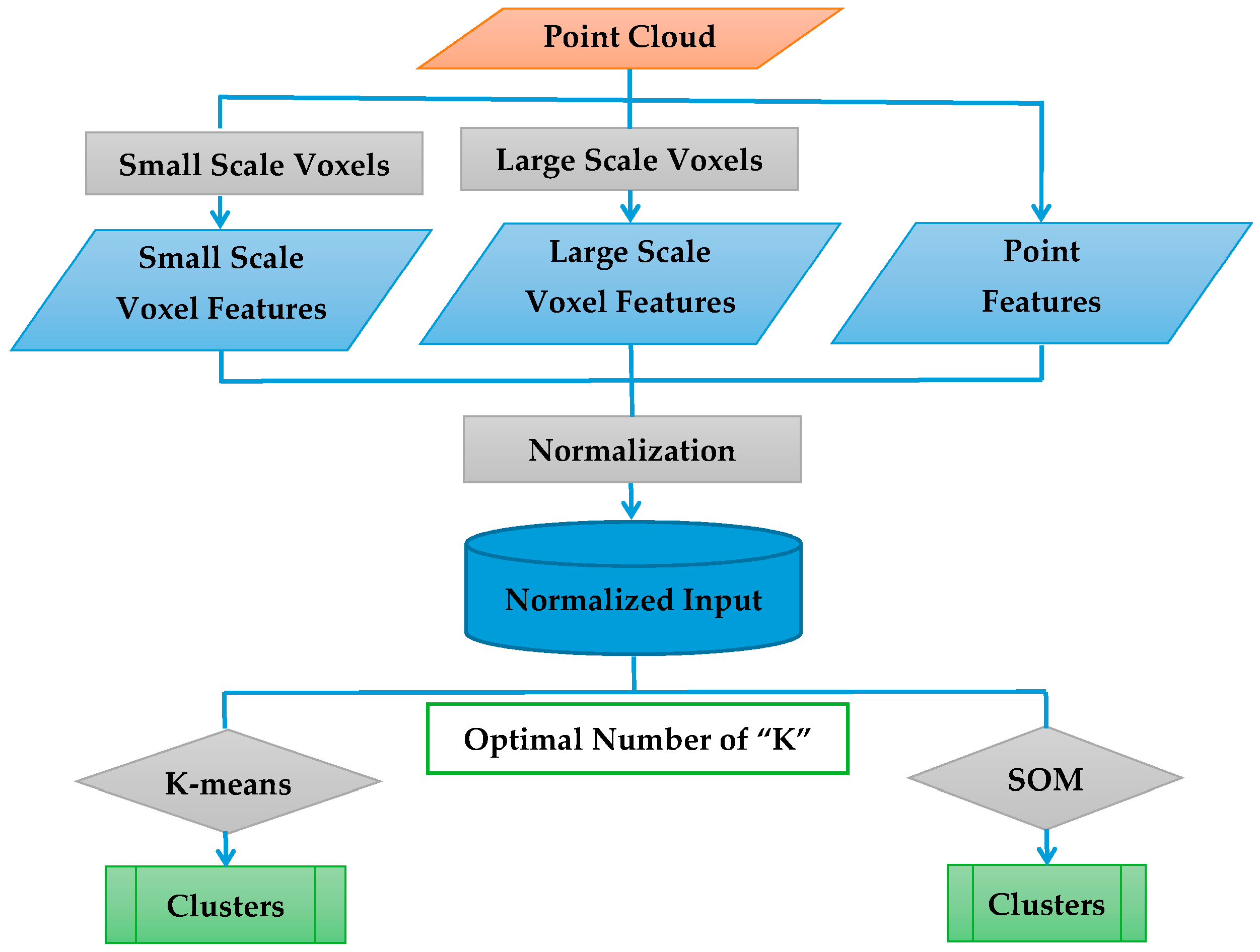
Figure 3 shows the flowchart of the developed method. The choice of features is one of the most important factors influencing the performance of the clustering algorithm. If the selected features represent the data well, the clusters are likely to be compact and separated and even a simple clustering algorithm such as K-means should identify a realistic segregation of the data set [36]. The main idea behind the novel framework presented here is to apply multi-scale voxel-based categorization of the 3D space to create a set of features that characterize the local complexity and geometry of the terrain. By “local geometry” it is meant how the information within the point cloud can be processed to indicate if the local geometry is more like a line (1D), a plane surface (2D), or whether points are distributed within the whole volume around the considered location (3D). For instance, at large scale, a power line can appear 1D; tidal flats can be represented as a 2D plane surface, while vegetation, such as Spartina spartinae mats in an upland area, can be distributed in the whole volume of a voxel and have a more 3D structure. Marsh surfaces and landcover are heterogeneous and their distinctive characteristics are seldom defined at a unique spatial scale, prompting the use of multi-scale criteria. When combining information from different scales, we have the potential to build signatures that better characterize marsh surface topology. Multi-scale voxelization can effectively characterize different types of vegetation as a small volume voxel will not store enough information to accurately extract features of a wide spread homogeneous area such as a tidal flat. A large capacity voxel will not capture more finely detailed objects such as the geometrical characteristics of different types of marsh vegetation. One of the main goals of this research is to identify a combination of features that is able to segment efficiently and accurately the marsh terrain at a high resolution. If features were only computed on the basis of voxels, clustering would be limited to the voxels and all points in a voxel would be assigned to the same cluster, regardless of the clustering algorithm. To address this effect, point-based characteristics are also included as part of the clustering algorithm input. TLS-based point features that reflect the characteristic of the surface such as elevation, relative reflectance and pulse waveform deviation were selected along with the per-voxel features. The latter two features, relative reflectance and pulse waveform deviation, are per-point measures recorded by Riegl’s V-line of scanners including the VZ-400 TLS used in this study. The selection of these features, or feature engineering, is described in Section 3.2. Furthermore, two clustering algorithms were evaluated: the well-known K-means (Section 3.4) and Self-Organizing Map (SOM) (Section 3.5) algorithms.
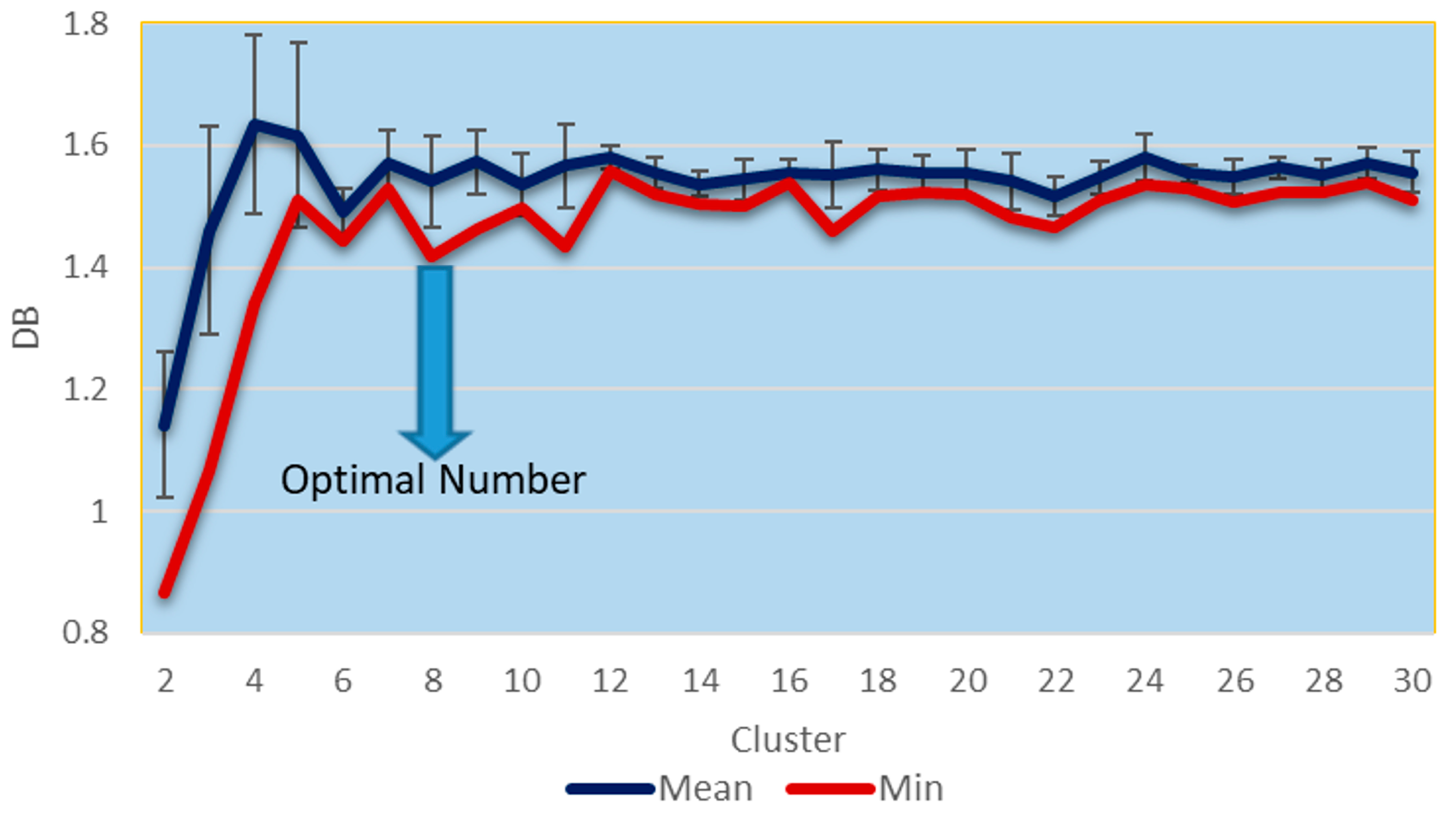
Another challenge with data clustering is determining the optimal number of clusters (“k”) that will best segment one’s data. While there may be some subjectivity depending on the level of details sought, the goal of this study was to develop an automated process. A method was sought that, when applied to TLS point cloud data, allows the extracted feature set to resolve clusters in an optimal way based on a given cost function. The result will be an “optimal” segmentation of the point cloud for the given set of features and clustering algorithm. The resulting number of clusters will vary depending on the marsh site and will be a reflection of the complexity of the scene, useful information in itself. For example, a marsh site with a small number of clusters should represent a less varied landscape such as mostly tidal flats while a marsh site resulting in many clusters may be populated by different types of vegetated areas. To determine the optimal number of clusters (optimal “k”) the Davies-Bouldin cluster evaluation criterion was implemented (See Section 3.3).
3.2. Feature Engineering
In this research, voxelization was not utilized as a segmentation technique as in earlier studies [37,38] but as a feature engineering technique. The following paragraphs describe the major function and steps of the methodology. First, the octree voxelization “splitting” process starts by using the whole data set as a root node. The data set space is repeatedly divided into 8 equal voxels until one of these three criterions is met: (1) the maximum number of points that a voxel can contain, (2) the minimum voxel dimension, or (3) the maximum number of subdivisions, usually referred to as voxel depth is reached. If a voxel has more points than allowed or a voxel’s dimension is larger than the minimum dimension, the voxel will be recursively subdivided until it reaches the maximum depth. In this experiment, the number of points in each voxel varied. The farther away from the scan center, the point density decreases and the voxel size adapts resulting in lower density voxels.
Two scales of voxels were used to create features from the segmented and octree filtered point cloud as described in Section 2.2 above. A fine scale was selected to match the size of a combination of a few vegetation species. Salt marsh plants such as Batis maritima at the study site are dioecious, perennial sub shrubs with heights in the range of 0.1–1.5 m and a span of 1–2 m for a group of plants. Therefore, to capture the different types of vegetation and marsh environmental features, a voxel size of 260 cm × 260 cm × 9 cm was selected. The 9 cm vertical range, smaller than the voxel’s lateral dimensions of 260 cm, was chosen to match the overall scene’s environments. For example, data from tidal flats are concentrated in thin vertical slices. In addition, voxel sizes smaller than 260 cm would result in many voxels containing less than the required minimum of at least 10 points to compute voxel-based statistics. The coarser scale voxels were selected to capture broader spatial scale differences between environment types, such as between tidal flats and vegetated areas. Tidal flats typically span several meters. To identify these more widely spread features, a voxel size of 530 cm × 530 cm × 18 cm was selected. For both voxel sizes, their respective dimensions are also driven by the initial point cloud aspect ratio, i.e., 340 cm × 340 cm × 10 m (340 m stems from the 170 m radial distance used to set the cloud extent described in Section 2.2 and 10 m represents the maximum height of representative features expected above ground level in the study area).
Once voxelization is applied, point cloud statistical features are computed to capture the variability within each voxel characteristic of differing terrain types or other scene features. The following set of five features is extracted for each fine and broader scale voxel: standard deviation of height (usually referred to as surface roughness), standard deviation of reflectance, standard deviation of waveform deviation, and two indexes referred to as curvature 1 and curvature 2 based on Principal Component Analysis (PCA) describing the general curvature of the point clouds within the voxels.
Standard deviations with the voxel points are calculated because they reflect the complexity of the terrain surface. When the standard deviation approaches one (assuming the feature is normalized), it indicates a very heterogeneous surface. When a voxel standard deviation approaches zero, it indicates that the surface is very homogeneous. For example, standard deviation of point height, , for a tidal flat will be smaller and closer to zero compared to a mixed vegetation area. The waveform deviation is an indicator of how clean the laser pulse reflection is coming back to the scanner relative to the outgoing laser pulse; the smaller the waveform deviation value, the less noise it contains. Similar to standard deviation of the point height, standard deviation of pulse waveform deviation for a tidal flat will be smaller and closer to zero compared to a mixed vegetation area that can generate a convolved, mixed signal waveform. The calibrated relative reflectance measure provided by Riegl’s V-line scanners is a ratio of the actual amplitude of that target to the amplitude of a white flat target at the same range, orientated orthonormal to the beam axis, and with a size in excess of the laser footprint. The actual reflectance reading is given in decibel (dB). Negative values hint to diffusely reflecting targets, whereas positive values are usually retro-reflecting targets. A relative reflectance higher than 0 dB generally results from targets, such as corner cubes or reflector foils, reflecting with a directivity different from that of a Lambertian reflector [39]. For a voxel containing a 3D point set, for i = 1, …, N number of points, the standard deviations of the point set’s height (surface roughness) is , point set’s relative reflectance value is , and point set’s waveform deviation value is , where x, y, and z are coordinate values.
Principal Components Analysis is a common statistical approach used to transform multi-variate data into linearly uncorrelated variables called principal components. Each variance value of the principal components corresponds to its eigenvalue [38]. The PCA technique is applied to the point cloud following the method developed by [38]. The variabilities in the morphometric structures (geometry) are analyzed by applying PCA to the 3D data within each voxel with the resulting eigenvalues derived from the covariance matrix [40]. For each voxel, three eigenvalues, ≥≥), are derived from the 3D point set of N points, (i = 1, …, N). quantifies the variance explained by the first dimension, while and do so for the second and third dimensions respectively. Curvature indexes are derived based on the eigenvalues with [41]. The largest curvature value,, is referred to as curvature 1. A voxel with a point cloud associated with a dominant value for ( ≈ 1 and ≈ 0), has a 1D-like distribution. If a voxel has = 0.5, and the geometry of this voxel can be characterized as a 2D-like surface, while a voxel with = 0.4, , and is characteristic of a 3D-like geometry. The study site is part of a salt marsh, and thus a goal of the clustering algorithm is to separate vegetation areas that have 3D-like distributions from tidal flats that have 2D-like distributions. The ratio of to is used to quantify such difference and is referred to as curvature 2 and expressed by Equation (1).
In addition, per point features were also extracted from the point cloud. These point features are height (elevation), Z, relative reflectance, R, and waveform deviation, D, as described above. Note that the point’s planar coordinates are not part of the selected features to favor segregation by environment type.
In summary, after the features are extracted, 13 different features characterize each point of the data set: 5 features for each small and broad scale voxelization (10 total) and 3 per-point features. These features have different dynamic range and units. Normalization is an essential preprocessing step in K-means and SOM clustering methods [42]. Both methods are based on minimizing the Euclidean distance between the data set points and cluster centroids, which are sensitive to differences in magnitude or scale of the features. Because of the differences in range in features’ values, one feature can overpower the other one. Normalization prevents the outweighing of some attributes and equalizes the magnitude and variability of all features by standardizing their values from different dynamic ranges into a specified range. There are three common normalization methods; they are Min-max, Z-score, and decimal scaling normalization [42]. In this research, we used Z-score to normalize the multiple features. In Z-score normalization, the values for a feature are normalized based on the mean and standard deviation of . For sample data with mean and sample standard deviation S, of a feature is computed as:
where:
3.3. Determination of the Number of Clusters
Many criteria have been proposed for determining an optimal number of clusters; examples are the Dunn, Calinski Harabasz, Silhouette, Gap, and Davies-Bouldin cluster criterions. These criteria have the common goal of identifying a number of clusters that result in compact well separated clusters and each has pros and cons in terms of applications. The Davies-Bouldin criterion was used in this research because of its reasonable performance in many clustering scenarios relative to more complex metrics [38], and the ability of the method to handle very large data sets with reasonable computing times on a high-performance desktop computer. The latter criteria is also advantageous for eventual real-time operation of an unsupervised clustering method for rapid 3D data segmentation based on the method presented here. The Davies-Bouldin index is a function of the ratio of the sum of within-cluster scatter to between-cluster separation [43]. The goal of the method is to find the number of clusters and data segregation that minimizes this index. The Davies-Bouldin index is defined as Equation (3) below.
where is the within-to-between cluster distance ratio for the ith and jth clusters,
and : the average distance between each point in the ith cluster and the centroid of the ith cluster. : the average distance between each point in the jth cluster and the centroid of the jth cluster. : the Euclidean distance between the centroids of the ith and jth clusters.
3.4. K-Means
In this research, we used K-means clustering, or Lloyd’s clustering algorithm [44], which is an iterative, data-partitioning algorithm that assigns each point of a data set to exactly one of k clusters with the clusters defined by their centroids and the optimal k determined by the Davies-Bouldin criterion. The K-means algorithm utilized here was implemented with Matlab and proceeds as follows:
- Compute point-to-cluster-centroid distances for full data set and for each centroid.
- Apply a two-phase iterative algorithm to minimize the sum of point-to-centroid distances, summed over all k clusters.
- Batch updates: each iteration consists of reassigning points to their nearest cluster centroid, all at once, followed by recalculation of cluster centroids. This phase occasionally does not converge to a solution that is a local minimum. That is, a partition of the data where moving any single point to a different cluster increases the total sum of distances.
- Online updates: points are individually reassigned if doing so reduces the sum of distances, and cluster centroids are recomputed after each reassignment. Each iteration during this phase consists of one pass through all the points. This phase converges to a local minimum. Finding the global minimum is solved by an exhaustive choice of starting points by using variety of replicates with random starting points typically resulting in a solution.
- Compute the average values in each cluster to obtain k new centroid locations.
- Repeat steps 2 through 4 until cluster assignments no longer change, or the maximum number of iterations is reached.
3.5. SOM
In addition to the K-means algorithm, the Kohonen’s Self Organizing Map [46,47] algorithm is used to identify underlying structure and natural patterns across the data set. The objective of a SOM is to map input data patterns onto a n-dimensional grid of neurons. That grid forms the output space, while the input space is the same set of features described above. Given the nonlinear functions of the neurons, SOM is capable of a more complex clustering geometry providing a valuable comparison for the relatively simpler K-means method. Another advantage of SOM over other clustering methods is the preservation of topological patterns, i.e., the organization of the map of clusters follows a pattern in the output space that is correlated with the progression of the input features most responsible for the resulting clustering. The SOM training algorithm can be described as follows:
- is the set of n training patterns ;
- is a grid of units where and are their coordinates on that grid;
- α is the learning rate, assuming values in , initialized to a given initial learning rate;
- r is the radius of the neighborhood function initialized to a given initial radius;
- Calculate for all with k = 1 to n.
- Select the unit that minimizes as the winner .
- Update each unit : .
- Decrease the value of α and r.
- Repeat steps 1–4 until α reaches 0.
SOM clustering for this work was performed in Matlab. The developed SOM network had one layer, with neurons organized in a grid. As explained further in Section 4 below, based on the Davies-Bouldin optimization criterion for K-means, the results showed that eight was an optimal number of clusters based on the given feature space and data set. Hence, to evaluate performance of the SOM algorithm relative to the K-means output, the SOM grid dimensions were specified as two rows by four columns, which created a total of eight neurons or clusters. The weight vector associated with each neuron moves to become the center of a cluster of input vectors. In addition, neurons that are adjacent to each other in the hexagon topology should also move close to each other in the input space because of the distance function between the neurons. Therefore, SOM is useful for visualizing a high-dimensional input space in the two dimensions of the network topology. The second important parameter in SOM is selecting training steps for initial covering of the input space. Here, it was specified as 1000 iterations with the initial neighborhood size of three, because the network provided consistent results at 1000 iterations.
4. Results and Discussion
4.1. Clustering Results
Using the data measured within a 170 m radius circle around the TLS scanner (see Section 2), K-means runs were performed to generate clusters based on all previously mentioned point and voxel features. Davies-Bouldin (DB) indexes were computed while increasing the number of clusters (2–30) and using the normalized features (see Section 3.2). For each cluster size, DB was computed for 50 replicates with a maximum of 1000 iterations. The mean and minimum DB values of the 50 replicates are plotted in Figure 4. The smallest DB values are obtained for two and three clusters because large inter-cluster distance values typically occur when the number of clusters is low for K-means [48]. However, a marsh surface is a complex and heterogeneous environment requiring a larger number of clusters to be properly described. Therefore, instead of simply selecting the k = 2 which leads to the minimum DB value as shown in Figure 4, a local minimum for k > 3 was selected based on the following rule [43]:
Here, was set to 30 clusters as we do not want, nor expect marsh landcover to require segmentation into more than 30 homogenous groups. As shown in Figure 4, k = 8 clusters was determined to be the local minimum DB value, , for k > 3. Note that the mean DB values are similar for k > 3 and that the selection of k = 8 was guided by the minimum DB value (Equation (5)) and the expected number of clusters given the main marsh features. Out of the 50 replication runs for k = 8, the run that derived the minimum DB value was selected as the K-means cluster solution for the eight clusters.
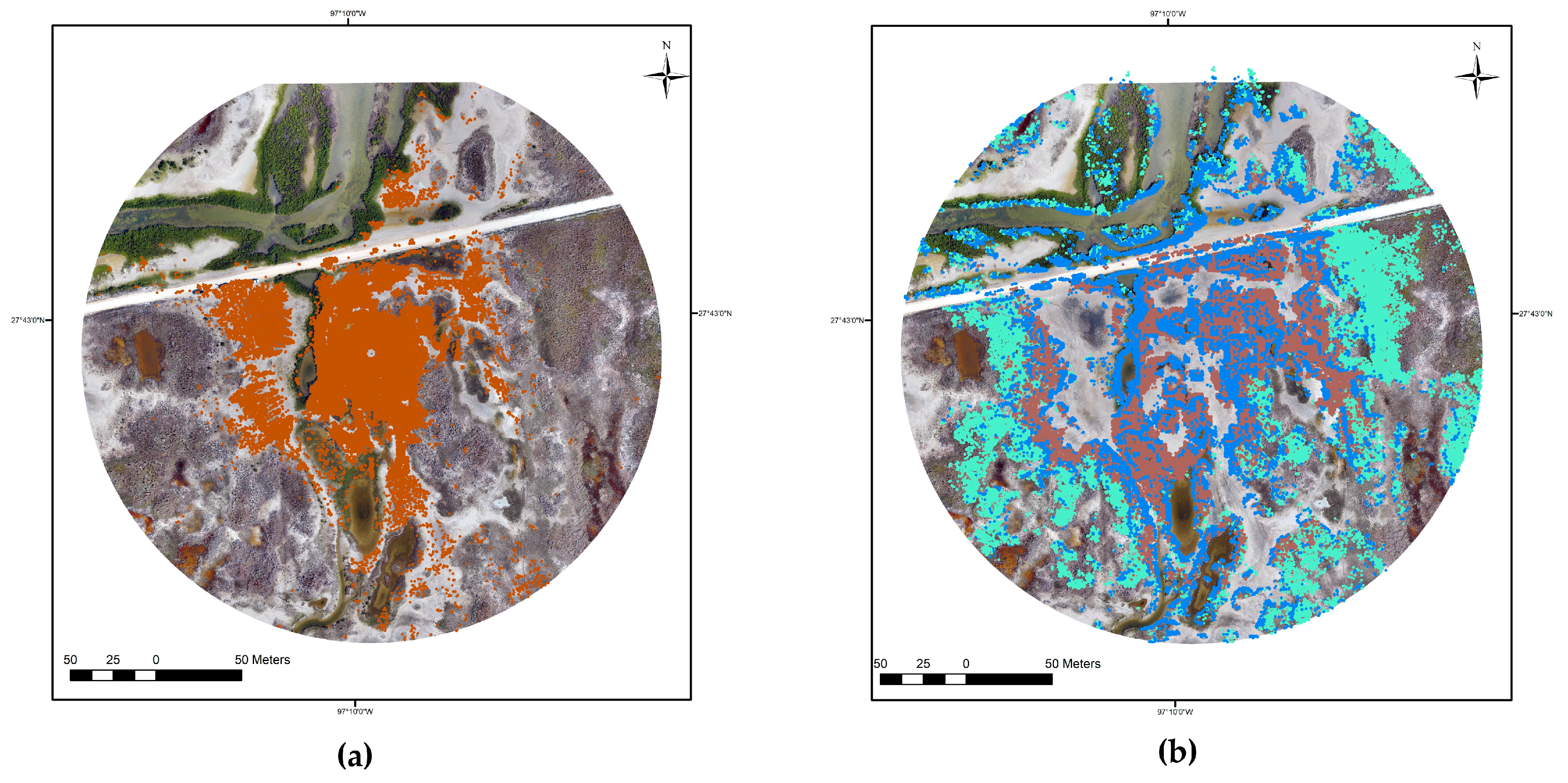
The main goal of this research is to use the clustering algorithm to identify patterns in the point cloud data and associate resultant clusters to marsh landcover features, such as exposed ground and vegetation points as well as other unforeseen patterns. Results for six of the selected eight clusters are presented in Figure 5. In Figure 5a the combined locations identified by three of the clusters are mapped. One can observe contiguous tidal flat areas surrounded by vegetated areas. In Figure 5b points identified by the combination of three other clusters are displayed. Vegetated areas surround the tidal flats as expected for a marsh with the vegetation pattern transitioning from low marsh, to high marsh, to upland. In Figure 5a the three clusters are identified as representing: high tidal flats, low tidal flats with sparring algal coverage and partially vegetated tidal flats. The three clusters illustrated in Figure 5b represent vegetated areas: Black Mangrove, low marsh to high marsh, and upland vegetation. The results show that the method segments different portions of the point cloud based on the selected computational features and captures well the natural pattern of the study area. An additional cluster captures the small portion (0.1%) of the point cloud belonging to a power line while the last cluster, only 0.2% of the point cloud, was spread across the study area and not directly identifiable.
Table 2 below further summarizes the cluster decomposition of the scene including the percentage of the entire point cloud included in each cluster. The results indicate that besides three tidal flat environments the developed method recognizes explicitly Black Mangrove but only identifies other vegetated areas as two aggregates: low marsh transition to high marsh and upland vegetation. It may be possible to identify more specifically individual vegetation types if the point cloud was segmented into more clusters.
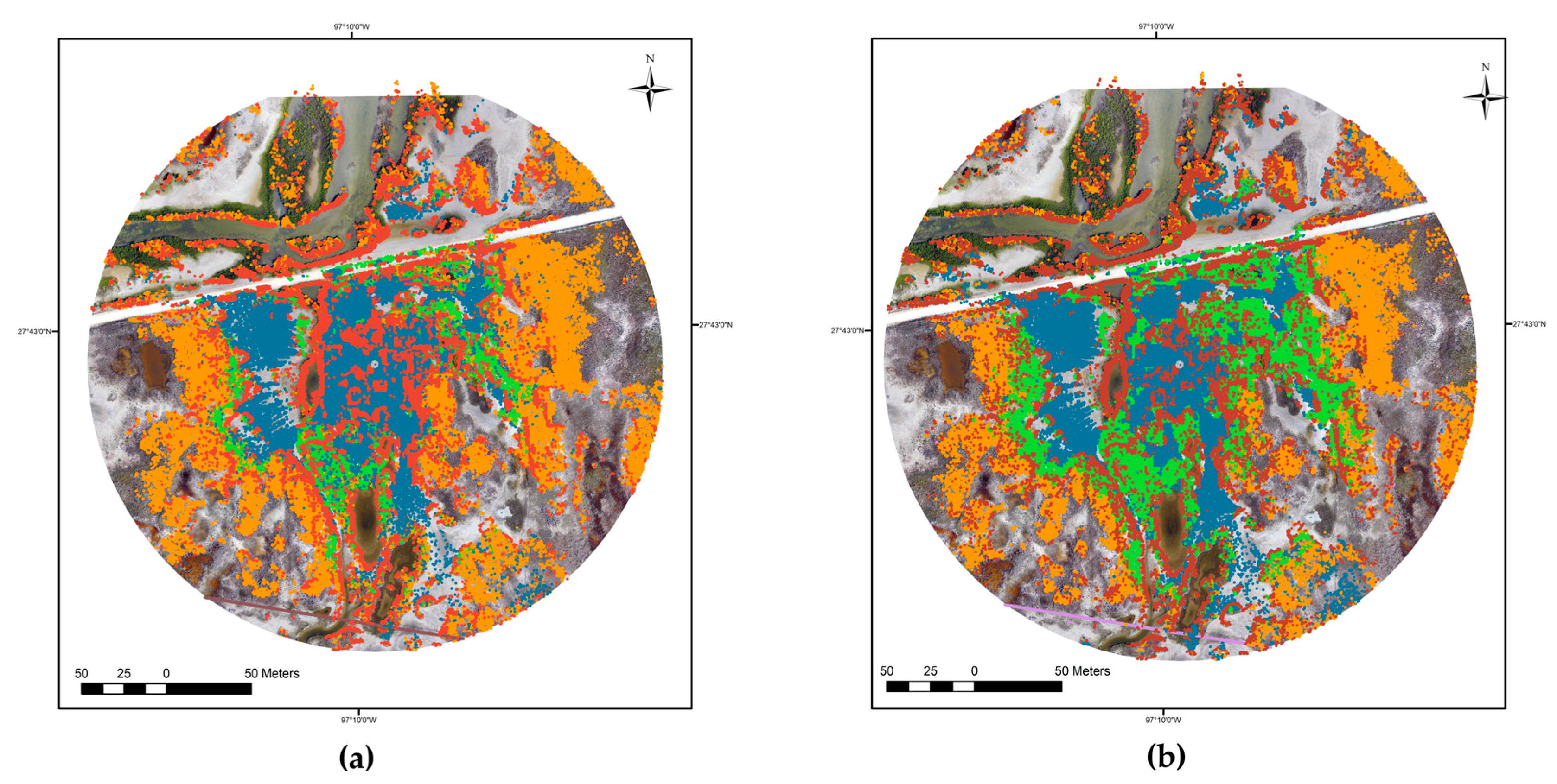
In Table 2 and in Figure 6, the K-means results are compared with the SOM segmentation. Overall, the SOM method partitions the study area in very similar clusters as compared to the K-means results. SOM identifies three tidal flat clusters but four vegetated clusters. Both K-means and SOM identify the presence of the power lines but SOM does not have an unidentified group of points spread across the scene and hence is a little more efficient in its clustering for this case. The number of points in each cluster, however, differ. K-means identifies about 61% of the point cloud as tidal flats while SOM assigns about 50%, both methods doing so in three tidal flat clusters: high flats, low flats with sparring algal coverage and partially vegetated flats. While K-means assigns more points to tidal flats than SOM, SOM assigns more points to its four vegetation clusters, including two clusters identified as low marsh transition to high marsh area. One of these two SOM clusters identifies the higher elevation portion of the marsh transition while the other cluster identifies the lower one. Hence, classification differences are for transition areas with vegetation density likely playing an important role. For example, K-means identifies transition zones with sparse vegetation as vegetated tidal flats while SOM identifies these same areas as transition from low to high marsh. Overall, K-means identifies about 17% of the point cloud as low marsh transition to high marsh area while SOM identifies about 30% of the point cloud as such. K-means and SOM identify virtually the same vegetated upland and mangrove areas in respective proportions of the point cloud of 10.4% vs. 9.5% and 10.8% vs. 9.3%. Overall, both methods performed well for the unsupervised identification of the main marsh areas, the different tidal flats and vegetated areas.
4.2. Classification Accuracy
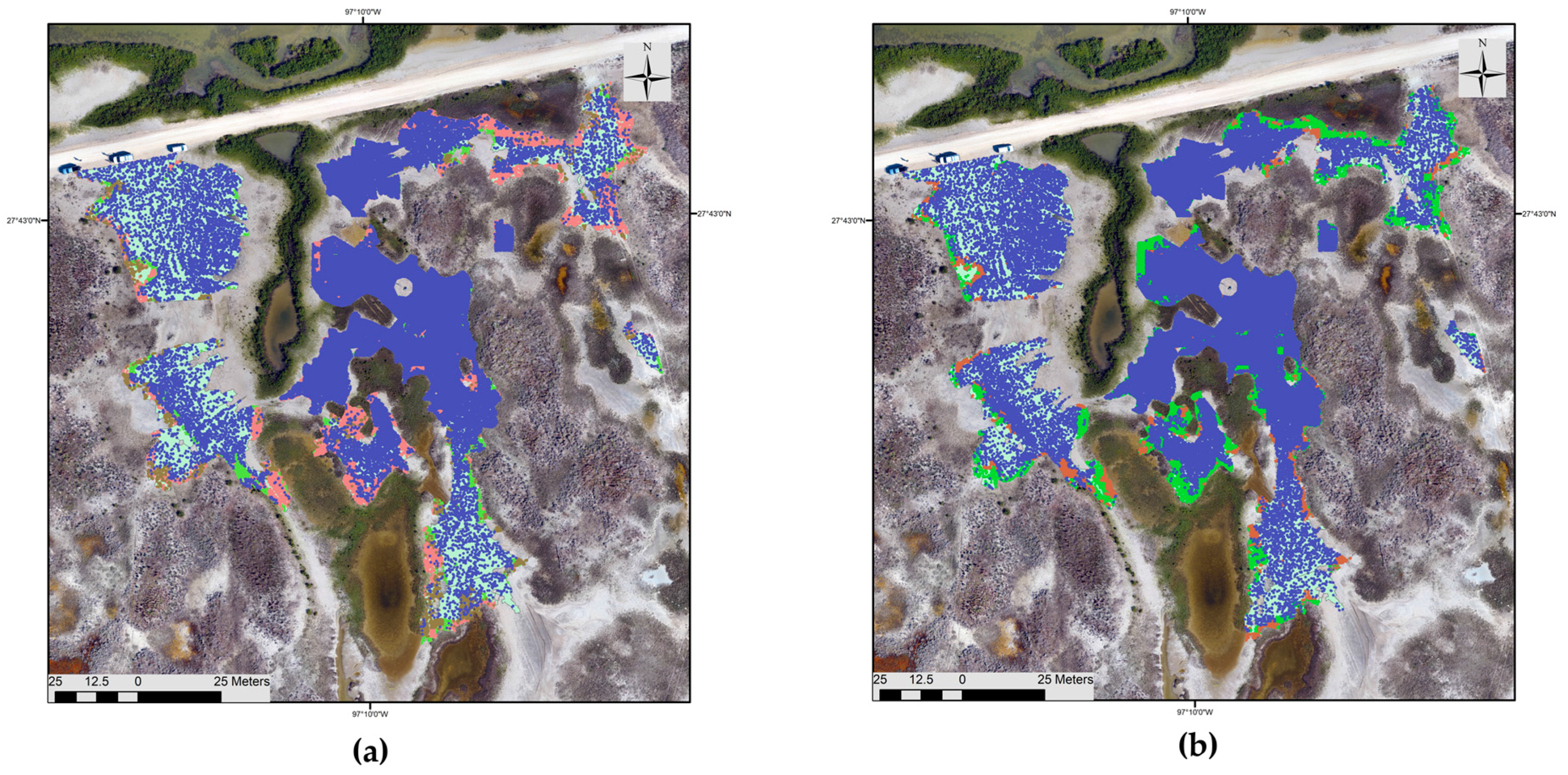
To further quantify the cluster partitioning and compare the methods, polygons for a portion of tidal flats in the study area were created and delineated from the co-aligned UAS imagery based on interpretation by a marsh expert. The polygons and clusters were overlaid in order to compute the number of tidal flat points that fall inside the polygons (Figure 7a,b) and estimate unsupervised classification error. The summary of the quantitative assessment for tidal flat is described in Table 3. Using K-means, about eighty-eight percent of all points falling inside the polygon are part of tidal flat clusters while about twelve percent are vegetation clusters. This corresponds to an approximate 12% error of omission for K-means tidal flat points. SOM results are similar to K-means; however, K-means results are slightly more accurate than SOM in identifying tidal flats. Using SOM, about eighty-five percent of all points falling inside the polygons are part of tidal flat clusters while about fifteen percent are part of vegetation clusters. This corresponds to an approximate 15% error of omission for SOM tidal flat points. Very few number of points falling inside the polygons are part of power line or mixed clusters; 0.1% for K-means and 0% for SOM, respectively.
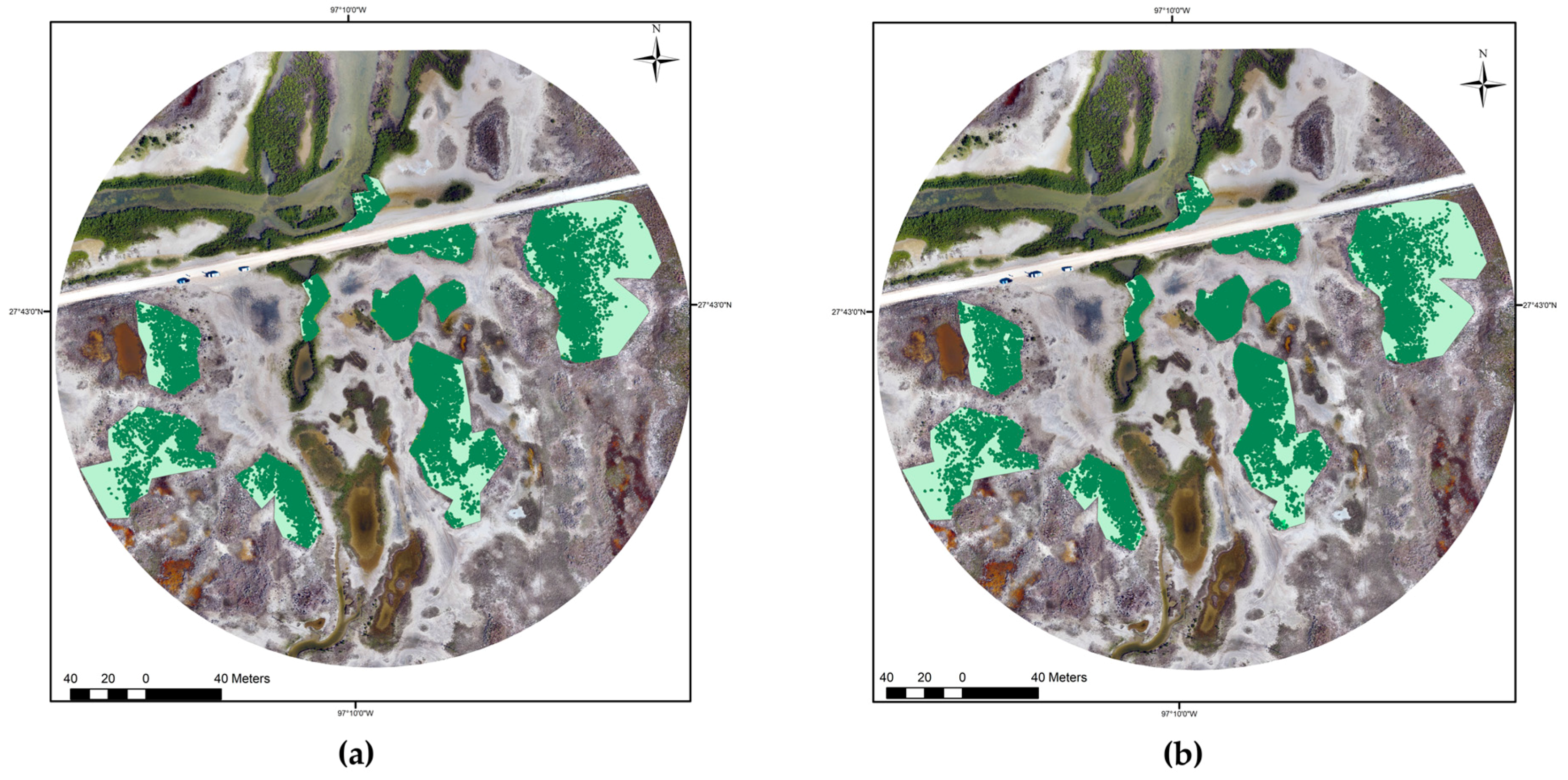
Similarly, polygons for a portion of vegetation areas in the study site were created and delineated from the co-aligned UAS imagery. The polygons and clusters were overlaid in order to compute the number of vegetation cluster points for K-means and SOM (refer back to Table 3 to see vegetation clusters) that fall inside the polygons (Figure 8a,b). Using K-means, about seventy percent of all points falling inside the polygon are part of vegetation clusters, while about thirty percent are tidal flat clusters. This corresponds to an approximate 30% error of omission for K-means vegetation points. In contrast, SOM results are more accurate than K-means in identifying vegetation areas. Using SOM, about ninety percent of all points falling inside the polygons are part of vegetation clusters while about ten percent are part of tidal flat clusters. This corresponds to an approximate 10% error of omission for SOM vegetation points. Zero percent of all points falling inside the polygons are part of power line or mixed clusters for both K-means and SOM.
Using both sets of polygons, the commission error was computed for tidal flats and vegetation. K-means had 17% commission error for tidal flats (vegetation points being committed to tidal flat points) and 23% for vegetation (tidal flat points being committed to vegetation points). In contrast, SOM had 7% commission error for tidal flats and 23% for vegetation.
Finally, a polygon for the road in the study area was created and delineated from the co-aligned UAS imagery. The road does not fall into tidal flat or vegetation landcover though one would expect it to more closely align with tidal flat due to it being an exposed surface. Interestingly, about 70% of all points falling inside the road polygon are part of vegetation clusters for K-means, and only about 30% of all points falling inside the road polygon are part of tidal flat clusters. Similarly, about 60% of all points falling inside the road polygon are part of vegetation clusters for SOM, and about 40% of all points falling inside the road polygon are part of tidal flat clusters. The potential reason for this apparent disparity is discussed further in Section 4.4 below.
4.3. Feature Importance
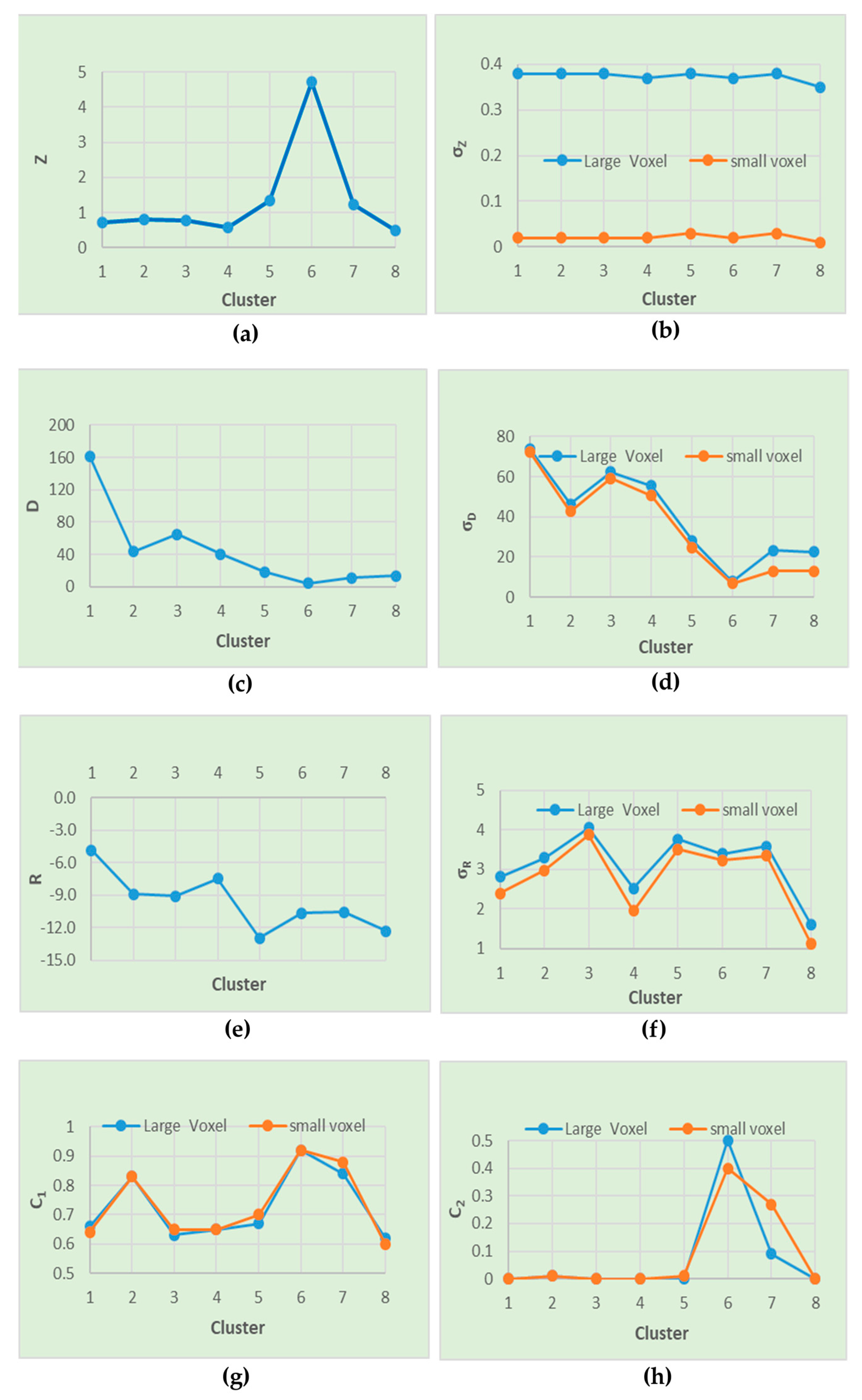
To assess the relative importance of the input features on the K-means clustering results, the means of each cluster were calculated and are illustrated in Figure 9. First, recall that these features were normalized by the Z-score, so they are unit-less and the closer to zero the values approach, the closer they are to the mean of the population. Second, the mean is examined across clusters for each individual feature. One of the important things learned from Figure 9 is that some features are significantly different for each particular cluster. For example, cluster 1 (vegetated tidal flat) has a substantially larger waveform deviation, D = 161.63, as compared to other clusters which have values of 65.09 or less. Cluster 6 (power line) has a large mean height value of 4.72 as compared to 1.33 or less for the other landcover clusters, which is expected. Some features best discriminate one group better than others. Furthermore, the standard error of the feature means for all clusters was computed. A small range in standard errors indicates that the data points in the cluster are close to the cluster centroid. Standard errors for the cluster feature means ranged from 0 to 0.79, which suggests that clusters are cohesive or compact.
Finally, the relative compactness of the feature distributions within their cluster assignments is quantified using the F statistic. The results are presented in Table 4. The F value is a ratio of variability between clusters over variability within a cluster [49]. Therefore, the larger the F value for a given feature relative to other features, the more differences (separable) it represents among the given clusters. Based on the F statistic, it shows that SOM and K-means have a different ranking on feature distinctness. However, they both reveal that the combination of features from multiple-scale voxel and individual points are important for a good clustering for the scene. Furthermore, the p-values of all F statistics for both of them are approximately zero indicating significant differences among the clusters but expected given the very large sample sizes.
For K-means, the largest F value is found for curvature 2 computed over the large voxels. The high value for this feature computed over the large scale voxels is likely due to the partitioning of most of the point cloud into tidal flats (2D like) and vegetation (more 3D like). The power line is a 1D-like feature but represents only about 0.1% of the point cloud. Behind the large voxel curvature 2, the next four most distinct features based on the F statistics are all computed over small voxels: surface roughness (standard deviation of Z), standard deviation of reflectance, curvature 2 and standard deviation of waveform deviation. The relative importance of the features computed over the small voxels suggests that capturing the small-scale variability of the marsh environment through feature engineering is important for a good clustering of the scene.
On the other hand, for SOM, the largest two F values are found for the standard deviation of reflectance and surface roughness (standard deviation of Z) computed over small voxels. The next four most distinct features are standard deviation of reflectance computed over large voxel, standard deviation of waveform deviation computed over small voxel, per-point waveform deviation, and the standard deviation of waveform deviation computed over large voxel. The high F values for these features show that the combination of both voxel and individual point features influence the SOM clustering. The relative importance of these features also suggests that both small and large voxel features help SOM segment the marsh environment.
For both K-means and SOM, the least distinctive features following the F statistics are the curvature 1 indexes computed for both small and large voxels. Looking at Table 4 one can also see that the curvature 1 values are not substantially different between clusters. While for this scene such features could be omitted, they should be kept for a general algorithm as curvature 1 has been shown to help identify buildings and other such structures [38]. The top features for K-means and SOM have relatively similar F values between 1,700,000 and 4,100,000 but display a different order likely related to differences in how the respective methods cluster the point cloud.
4.4. Discussion
Considering the developed method is a completely unsupervised clustering, the accuracy results presented in Section 4.2 suggest that K-means and SOM are able to identify with reasonable accuracy tidal flat among different marsh environments without supervised training. Similarly, the accuracy results for vegetated landcover segmentation are promising as well. However, in this case, SOM outperformed K-means rather substantially suggesting SOM may be more suitable for vegetation discrimination. This could be a case where the nonlinear functions of the neurons in the SOM provided an advantage for handling more complex clustering geometry represented by the marsh’s highly varying vegetated landcover. In regard to evaluation of points along the road, results showed that the majority of points for both K-means and SOM were stemming from the vegetation clusters, not tidal flat clusters as expected. Although unexpected to have majority vegetation, it is likely due to the road being elevated relative to the lower lying tidal flats. Elevation (Z) is one of the per-point input features and has strong control on marsh landcover transition so perhaps that had some influence here. Furthermore, the road has lots of ruts and gravel in parts providing a higher surface roughness compared to a tidal flat surface. This may also play a role in points going towards vegetation clusters. Finally, the road was only sparsely sampled and perhaps with denser sampling the segmentation could be different.
The disadvantage of a single scan, as utilized here, is that point density decreases radially away from the TLS and vegetation occlusion plays a major role. To account for the radial decrease in point density, an octree filter was applied (Section 2.2) to try and better regularize the point density prior to clustering. However, this only affects areas of high density near the scanner. Variability in point density can affect the clustering results because the voxel’s features are derived from characteristics of all the points falling inside the voxel. The more points they have, the more detailed and accurate can a voxel at a certain size provide about the terrain. One way to potentially control this is to use a weighted voxelization that adapts to a set density, but over low-density areas, the voxel must grow to account for a drop-in density, which impacts spatial scale. Exploring the impact of point density on the clustering results is an interesting problem. To do so, multiple scan positions could be acquired and merged to provide a more homogeneous point density throughout the study area. This would enable comparison of clustering performance between a single scan (e.g., validating accuracy at certain distances radially away from the scanner) versus more uniform density from multiple scan positions. A relationship between decrease in point density and impact on cluster preservation of marsh environments could be explored. Furthermore, a merged point cloud of the study area could also be iteratively down sampled to try and parameterize how changes in density influence the clustering results.
In this work, the number of clusters was guided by the DB optimized k solution. This was done to reduce user subjectivity and provide an automated clustering based on an optimization criterion. The method could lead to different numbers of k for different marsh sites, which potentially relates to the complexity of the environment as captured by the TLS point cloud (i.e., >k implies a more complex landscape). However, this work represents only one marsh study site, and more research is needed to perform similar analysis at other marsh environments to fully determine the potential of the method. Furthermore, other metrics to determine the optimal k can lead to different number of k, and the choice of an optimization criterion is problem specific and data dependent as each metric has advantages and disadvantages. As an alternative approach, a tidal flat expert could iteratively tune the number of clusters going from smallest to largest using either K-means or SOM to achieve a desired clustering solution. For example, increasing the number of clusters could potentially resolve points on the dirt road as a separate cluster relative to vegetation or tidal flat areas. For such an approach, SOM provides an advantage in that the organization of the cluster map is correlated with the progression of the input features most responsible for the resulting clustering. This preservation of topological patterns could enable a novel way to explore connections between features and segmentation of different marsh environments. By increasing the size of the SOM grid, such information could be exploited to manually prune the number of clusters in an intelligent way to achieve a desired cluster solution.
Finally, the method was only sparingly tested for more clusters in part due to the following limitations. In a marsh environment, it is challenging to distinguish between individual types of vegetation. The plants within high marsh and low marsh environments, such as Bastis maritima, Monanthocloe litorals, and Saliconrnia are very similar in size, shape, surface roughness and reflectivity. The voxel size would need to be small enough to capture small differences in individual plant characteristics. The utilized fine voxel scale, 260 cm × 260 cm × 9 cm, is considerably larger than these plants’ foliage. Implementing a smaller voxel size would result in many voxels with insufficient number of data points, particularly in areas farther from the scanner. This limitation could be addressed by considering only data points acquired from a smaller radius around the scanner and the measurements being repeated at several locations. For future research, it may be interesting to explore the developed method with more clusters and/or smaller voxel sizes for higher point density scenes, such as a merged point cloud from multiple scan positions as suggested above.
5. Conclusions
A three-dimensional point cloud of a marsh measured with TLS was partitioned using unsupervised clustering methods. The developed method is able to identify the natural structure of a marsh environment with no prior training and to categorize millions of unlabeled data points into meaningful groups. At eight clusters, it identifies tidal flats, mangrove, low marsh to high marsh vegetation, upland vegetation, and even power lines representing only 0.1 percent of the point data. Results from K-means and SOM are very similar; they suggest that the selected features are robust and represent the data set well. Curvature of the eigenvalues of the planar surface greatly influenced K-means clustering results. Fine and coarser scale voxel features were identified as important for both the K-means and SOM clustering process, which suggests that the multi-scale voxelization efficiently captured the complexity and geometry of the marsh surface. The quantitative assessment results are acceptable, 88% of points within tidal clusters are indeed within tidal flats for K-means and 85% for SOM based on comparison to tidal flat area delineated from UAS imagery. K-means provides slightly better results in identifying tidal flats as compared to SOM but the optimizations are based on K-means instead of SOM. In contrast, 70% of points within vegetation clusters are indeed within vegetation for K-means and 90% for SOM based on comparison to vegetation area delineated from UAS imagery. Results suggest that SOM may be better able to handle more complex geometry of the vegetation areas. In the future, optimizations will be applied for both K-means and SOM. Davies-Bouldin index is efficient in determining the optimal number of clusters but it only provides guidance as differences in the index values are small. Intra-cluster and Inter-cluster assessment results show that the clusters are compact and well separated for both SOM and K-means. Overall, results demonstrate that the developed multi-scale voxelization approach and representative feature set are transferrable to other clustering algorithms, thereby providing an unsupervised framework for intelligent scene segmentation of TLS point cloud data in marshes. However, it is important to emphasize that adequate voxel size and feature performance could be different for different marsh regimes depending on the characteristics and geometry of the marsh surface as well as characteristics of the TLS data itself. Future work will explore the application of this method at different marsh regimes of varying terrain and landcover.
Acknowledgments
This publication was made possible through support provided by United States Department of Commerce—National Oceanic and Atmospheric Administration (NOAA) through The University of Southern Mississippi under the terms of Agreement No. NA13NOS4000166. The authors would like to thank the anonymous reviewers for their constructive comments and edits. The authors also gratefully acknowledge Alistair Lord, Brian Lorentson, Jacob Berryhill, and James Rizzo of the Conrad Blucher Institute for Surveying and Science at Texas A&M University-Corpus Christi for their fieldwork support and contributions.
Author Contributions
C.N. and M.J.S. conceived and designed the clustering framework with input from P.T.; C.N. developed the computational code, performed the experiments, and analyzed the results; M.J.S. and P.T. helped with algorithm development and results interpretation; J.G. provided guidance on marsh site selection, experimental design, and results interpretation; C.N. wrote the paper with assistance from M.J.S. and P.T.
Conflicts of Interest
The authors declare no conflict of interest.
References
- Barier, E.B.; Hacker, S.D.; Kennedy, C.; Koch, E.W.; Stier, A.C.; Silliman, B.R. The value of estuarine and coastal ecosystem services. Ecol. Monogr. 2011, 81, 169–193. [Google Scholar] [CrossRef]
- Boesh, D.F.; Turner, R.E. Dependence of fishery species on salt marshes: The role of food and refuge. Estuaries 1984, 7, 460–468. [Google Scholar] [CrossRef]
- Mitsch, W.J.; Gosselink, J.G. The value of wetlands: Importance of scale and landscape setting. Ecol. Econ. 2000, 35, 25–33. [Google Scholar] [CrossRef]
- Moor, H.; Hylander, K.; Norberg, J. Predicting climate change effects on wetland ecosystem services using species distribution modeling and plant functional traits. AMBIO 2015, 44, 113–126. [Google Scholar] [CrossRef] [PubMed]
- Costanza, R.; Pérez-Maqueo, O.; Martinez, M.L.; Sutton, P.; Anderson, S.J.; Mulder, K. The Value of Coastal Wetlands for Hurricane Protection. AMBIO 2008, 37, 241–248. [Google Scholar] [CrossRef]
- Pennings, S.C.; Callaway, R.M. Salt Marsh Plant Zonation: The Relative Importance of Competition and Physical Factors. Ecology 1992, 73, 681–690. [Google Scholar] [CrossRef]
- Silvestri, S.; Defina, A.; Marani, M. Tidal regime, salinity and salt marsh plant zonation. Estuar. Coast. Shelf Sci. 2005, 62, 119–130. [Google Scholar] [CrossRef]
- Suchrow, S.; Jensen, K. Plant Species Responses to an Elevational Gradient in German North Sea Salt Marshes. Wetlands 2010, 30, 735–746. [Google Scholar] [CrossRef]
- Church, J.A.; White, N.J. A 20th century acceleration in global sea-level rise. Geophys. Res. Lett. 2006, 33, 1944–8007. [Google Scholar] [CrossRef]
- NASA. Sea Level. Available online: https://climate.nasa.gov/vital-signs/sea-level/ (accessed on 9 September 2017).
- Warner, N.N.; Tissot, P.E. Storm flooding sensitivity to sea level rise for Galveston Bay, Texas. Ocean Eng. 2012, 44, 23–32. [Google Scholar] [CrossRef]
- Passeri, D.L.; Hagen, S.C.; Medeiros, S.C.; Bilskie, M.V.; Alizad, K.; Wang, D. The dynamic effects of sea level rise on low-gradient coastal landscapes: A review. Earths Future 2015, 3, 159–181. [Google Scholar] [CrossRef]
- Lemmens, M. Terrestrial Laser Scanning. In Geo-Information: Technologies, Applications and the Environment; Springer: Dordrecht, The Netherlands, 2011; pp. 101–121. [Google Scholar]
- Lichti, D.; Pfeifer, N.; Maas, H.-G. ISPRS Journal of Photogrammetry and Remote Sensing Theme Issue “Terrestrial Laser Scanning”; Elsevier: Amsterdam, The Netherlands, 2008. [Google Scholar] [CrossRef]
- Moorthy, I.; Miller, J.R.; Hu, B.; Chen, J.; Li, Q. Retrieving crown leaf area index from an individual tree using ground-based LiDAR data. Can. J. Remote Sens. 2008, 34, 320–332. [Google Scholar] [CrossRef]
- Straatsma, M.; Warmink, J.J.; Middelkoop, H. Two novel methods for field measurements of hydrodynamic density of floodplain vegetation using terrestrial laser scanning and digital parallel photography. Int. J. Remote Sens. 2008, 29, 1595–1617. [Google Scholar] [CrossRef]
- Buckley, S.J.; Howell, J.; Enge, H.; Kurz, T. Terrestrial laser scanning in geology: Data acquisition, processing and accuracy considerations. J. Geol. Soc. 2008, 165, 625–638. [Google Scholar] [CrossRef]
- Rosser, N.; Petley, D.; Lim, M.; Dunning, S.; Allison, R. Terrestrial laser scanning for monitoring the process of hard rock coastal cliff erosion. Q. J. Eng. Geol. Hydrogeol. 2005, 38, 363–375. [Google Scholar] [CrossRef]
- Starek, M.J.; Mitasova, H.; Hardin, E.; Weaver, K.; Overton, M.; Harmon, R.S. Modeling and analysis of landscape evolution using airborne, terrestrial, and laboratory laser scanning. Geosphere 2011, 7, 1340–1356. [Google Scholar] [CrossRef]
- Starek, M.J.; Mitásová, H.; Wegmann, K.; Lyons, N. Space-time cube representation of stream bank evolution mapped by terrestrial laser scanning. IEEE Geosci. Remote Sens. Lett. 2013, 10, 1369–1373. [Google Scholar] [CrossRef]
- Heritage, G.; Hetherington, D. Towards a protocol for laser scanning in fluvial geomorphology. Earth Surf. Process. Landf. 2007, 32, 66–74. [Google Scholar] [CrossRef]
- Milan, D.J.; Heritage, G.L.; Hetherington, D. Application of a 3D laser scanner in the assessment of erosion and deposition volumes and channel change in a proglacial river. Earth Surf. Process. Landf. 2007, 32, 1657–1674. [Google Scholar] [CrossRef]
- Harman, C.J.; Lohse, K.A.; Troch, P.A.; Sivapalan, M. Spatial patterns of vegetation, soils, and microtopography from terrestrial laser scanning on two semiarid hillslopes of contrasting lithology. J. Geophys. Res. Biogeosci. 2014, 119, 163–180. [Google Scholar] [CrossRef]
- Feliciano, E.A.; Wdowinski, S.; Potts, M.D. Assessing mangrove above-ground biomass and structure using terrestrial laser scanning: A case study in the Everglades National Park. Wetlands 2014, 34, 955–968. [Google Scholar] [CrossRef]
- Guarnieri, A.; Vettore, A.; Pirotti, F.; Menenti, M.; Marani, M. Retrieval of small-relief marsh morphology from terrestrial laser scanner, optimal spatial filtering, and laser return intensity. Geomorphology 2009, 113, 12–20. [Google Scholar] [CrossRef]
- Hladik, C.; Alber, M. Accuracy assessment and correction of a LIDAR-derived salt marsh digital elevation model. Remote Sens. Environ. 2012, 121, 224–235. [Google Scholar] [CrossRef]
- Hladik, C.; Schalles, J.; Alber, M. Salt marsh elevation and habitat mapping using hyperspectral and lidar data. Remote Sens. Environ. 2013, 139, 318–330. [Google Scholar] [CrossRef]
- Bowen, Z.H.; Waltermire, R.G. Evaluation of light detection and ranging (lidar) for measuring river corridor topography. J. Am. Water Resour. Assoc. 2002, 38, 33–41. [Google Scholar] [CrossRef]
- Chasmer, L.; Hopkinson, C.; Treitz, P. Investigating laser pulse penetration through a conifer canopy by integrating airborne and terrestrial lidar. Can. J. Remote Sens. 2006, 32, 116–125. [Google Scholar] [CrossRef]
- Pirotti, F.; Guarnieri, A.; Vettore, A. Ground filtering and vegetation mapping using multi-return terrestrial laser scanning. J. Photogramm. Remote Sens. 2013, 76, 56–63. [Google Scholar] [CrossRef]
- Wang, M.; Tseng, Y.H. Incremental segmentation of LiDAR point clouds with an octree-structured voxel space. Photogramm. Rec. 2011, 26, 32–57. [Google Scholar] [CrossRef]
- Paine, J.G.; White, W.A.; Smyth, R.C.; Andrews, J.R.; Gibeaut, J.C. Mapping coastal environments with LiDAR and EM on Mustang Island, Texas, US. Lead. Edge 2004, 23, 894–898. [Google Scholar] [CrossRef]
- Raber, G.T.; Jensen, J.R.; Hodgson, M.E.; Tullis, J.A.; Davis, B.A.; Berglund, J. Impact of LiDAR nominal post-spacing on DEM accuracy and flood zone delineation. Photogramm. Eng. Remote Sens. 2007, 73, 793–804. [Google Scholar] [CrossRef]
- Perroy, R.L.; Bookhagen, B.; Asner, G.P.; Chadwick, O.A. Comparison of gully erosion estimates using airborne and ground-based LiDAR on Santa Cruz Island, California. Geomorphology 2010, 118, 288–300. [Google Scholar] [CrossRef]
- Douillard, B.; Underwood, J.; Kuntz, N.; Vlaskine, V.; Quadros, A.; Morton, P.; Frenkel, A. On the Segmentation of 3D LIDAR Point Clouds. In Proceedings of the 2011 IEEE International Conference on Robotics and Automation (ICRA), Shanghai, China, 9–13 May 2011; pp. 2798–2805. [Google Scholar]
- Jain, A.K. Data clustering: 50 years beyond K-means. Pattern Recognit. Lett. 2010, 31, 651–666. [Google Scholar] [CrossRef]
- Brodu, N.; Lague, D. 3D terrestrial LiDAR data classification of complex natural scenes using a multi-scale dimensionality criterion: Applications in geomorphology. ISPRS J. Photogramm. Remote Sens. 2012, 68, 121–134. [Google Scholar] [CrossRef] [Green Version]
- Wakita, T.; Susaki, J. Multi-Scale-based Extraction of Vegetation from Terrestrial LiDAR Data for Assessing Local Landscape. ISPRS Ann. Photogramm. Remote Sens. Spat. Inf. Sci. 2015, 2, 263. [Google Scholar] [CrossRef]
- Pirotti, F.; Guarnieri, A.; Vettore, A. Vegetation filtering of waveform terrestrial laser scanner data for DTM production. Appl. Geomat. 2013, 5, 311–322. [Google Scholar] [CrossRef]
- Vandapel, N.; Huber, D.F.; Kapuria, A.; Hebert, M. Natural terrain classification using 3-D ladar data. In Proceedings of the IEEE International Conference on Robotics and Automation (ICRA’04), New Orleans, LA, USA, 26 April–1 May 2004; pp. 5117–5122. [Google Scholar]
- Carlberg, M.; Gao, P.; Chen, G.; Zakhor, A. Classifying urban landscape in aerial LiDAR using 3D shape analysis. In Proceedings of the 16th IEEE International Conference on Image Processing (ICIP), Cairo, Egypt, 7–10 November 2009; pp. 1701–1704. [Google Scholar] [CrossRef]
- Visalakshi, N.K.; Thangavel, K. Impact of normalization in distributed K-means clustering. Int. J. Soft Comput. 2009, 4, 168–172. [Google Scholar]
- Davies, D.L.; Bouldin, D.W. A cluster separation measure. IEEE Trans. Pattern Anal. Mach. Intell. 1979, 224–227. [Google Scholar] [CrossRef]
- Lloyd, S. Least squares quantization in PCM. IEEE Trans. Inf. Theory 1982, 28, 129–137. [Google Scholar] [CrossRef]
- Arthur, D.; Vassilvitskii, S. K-means++: The advantages of careful seeding. In Proceedings of the Eighteenth Annual ACM-SIAM Symposium on Discrete Algorithms; Society for Industrial and Applied Mathematics: Philadelphia, PA, USA, 2007; pp. 1027–1035. [Google Scholar]
- Kohonen, T. Analysis of a simple self-organizing process. Biol. Cybern. 1982, 44, 135–140. [Google Scholar] [CrossRef]
- Kohonen, T. Essentials of the self-organizing map. Neural Netw. 2013, 37, 52–65. [Google Scholar] [CrossRef] [PubMed]
- Ray, S.; Turi, R.H. Determination of number of clusters in K-means clustering and application in colour image segmentation. In Proceedings of the 4th International Conference on Advances in Pattern Recognition and Digital Techniques, Calcutta, India, 28–31 December 1999; pp. 137–143. [Google Scholar]
- Montgomery, D.C.; Runger, G.C.; Hubele, N.F. Engineering Statistics; John Wiley & Sons: Hoboken, NJ, USA, 2009. [Google Scholar]
Figure 1.
Study area at Mustang Island Wetland Observatory. The circular image overlaid on the satellite image is the study location. This area is shown in more detail in Figure 2 below.
Figure 1.
Study area at Mustang Island Wetland Observatory. The circular image overlaid on the satellite image is the study location. This area is shown in more detail in Figure 2 below.

Figure 2.
Study area at Mustang Island Wetland Observatory on 14 March 2017. (a) Aerial image overlaid on background image was acquired from a small unmanned aircraft system (UAS), DJI Phantom 4, equipped with a 12.4 MP RGB camera; (b) study site from ground view showing part of the tidal flat area and vegetated landcover.

Figure 3.
Flowchart of the developed method.

Figure 4.
DB index values: DB mean with standard error and DB minimum.

Figure 5.
K-means clustering results (a) tidal flat clusters (b) vegetated area clusters overlaid on UAS imagery.
Figure 5.
K-means clustering results (a) tidal flat clusters (b) vegetated area clusters overlaid on UAS imagery.

Figure 6.
Clustering results of (a) K-means and (b) SOM overlaid on UAS imagery. All clusters shown. Variability in point density and occlusion stemming mostly from vegetation for a single TLS scan position can also be observed.
Figure 6.
Clustering results of (a) K-means and (b) SOM overlaid on UAS imagery. All clusters shown. Variability in point density and occlusion stemming mostly from vegetation for a single TLS scan position can also be observed.

Figure 7.
Quantitative assessments of K-means and SOM in identifying tidal flat. Aerial image is from the UAS. (a) K-means results overlaid over the polygon; (b) SOM results overlaid over the polygon.
Figure 7.
Quantitative assessments of K-means and SOM in identifying tidal flat. Aerial image is from the UAS. (a) K-means results overlaid over the polygon; (b) SOM results overlaid over the polygon.

Figure 8.
Quantitative assessments of K-means and SOM in identifying vegetation. Aerial image is from the UAS. (a) K-means results overlaid over the polygon; (b) SOM results overlaid over the polygon.
Figure 8.
Quantitative assessments of K-means and SOM in identifying vegetation. Aerial image is from the UAS. (a) K-means results overlaid over the polygon; (b) SOM results overlaid over the polygon.

Figure 9.
Comparisons of feature means by cluster (a) point’s height, , (b) standard deviation of height for small and large voxels, , (c) point’s waveform deviation, , (d) standard deviation of waveform deviation for small and large voxels, , (e) point’s relative reflectance, R, (f) standard deviation of reflectance for small and large voxels, , (g) curvature 1 for small and large voxels, and (h) curvature 2 for small and large voxels, . Feature values shown are normalized.


Table 1.
Riegl VZ-400 factory specifications.
| Parameters | Specifications |
|---|---|
| Pulse repetition rate | Up to 300,000 kHz |
| Laser wavelength | 1550 nm |
| Beam divergence | 0.3 mrad |
| Spot size | 3 cm at 100 m distance |
| Range | 1.5 m (min), 600 m (max) * |
| Field of view | 100° vertical × 360° horizontal |
| Repeatability | 3 mm (1 sigma @ 100 m range) |
| Minimum stepping angle | 0.0024° |
* for natural targets with reflectivity >90%.
Table 2.
Summary of K-means and SOM cluster results for k = 8 clusters based on the optimized DB solution. The first column shows the cluster numbers for K-means and SOM that were identified for each marsh environment. Multiple clusters identifying tidal flats area (K-means and SOM) and low marsh to high marsh area (SOM) were regrouped into combined clusters. The percentages represent the portion of the points assigned to an environment for K-means and SOM based on a total of 9,511,286 points in the TLS point cloud.
| Marsh Environment | Cluster Numbers | Percentage (%) | ||
|---|---|---|---|---|
| K-Means | SOM | K-Means | SOM | |
| Tidal flats (high flats, low flats with sparing algal coverage, partially vegetated flats) | 1, 4, 8 | 1, 4, 8 | 61.2 | 50.3 |
| Black Mangrove vegetation | 2 | 2 | 10.8 | 9.3 |
| Low marsh to high marsh vegetation | 3 | 5, 7 | 17.2 | 30.7 |
| Upland vegetation | 5 | 6 | 10.4 | 9.5 |
| Power line | 6 | 3 | 0.1 | 0.2 |
| Mixed | 7 | 0.3 | ||
| Total | 100 | 100 | ||
Table 3.
Summary of the quantitative assessments for K-means and SOM in identifying tidal flats. The first column shows the cluster numbers for K-means and SOM that were identified for each marsh environment. The percentages represent the portion of the points for an environment that fell within the tidal flat polygons based on a total of 3,706,708 points. Clusters 1, 4, 8 for both K-means and SOM represent tidal flat area, and the percentages shown for those clusters represent the unsupervised classification accuracy for tidal flat.
| Marsh Environment | Cluster | Percentage | ||
|---|---|---|---|---|
| K-Means | SOM | K-Means | SOM | |
| Tidal flats (high flats, low flats with sparing algal coverage, partially vegetated flats) | 1, 4, 8 | 1, 4, 8 | 88.3 | 84.6 |
| Black Mangrove vegetation | 2 | 2 | 5.0 | 2.4 |
| Low marsh to high marsh vegetation | 3 | 5, 7 | 6.4 | 12.9 |
| Upland vegetation | 5 | 6 | 0.2 | 0.1 |
| Power line | 6 | 3 | 0.0 | 0.0 |
| Mixed | 7 | 0.1 | ||
| Total | 100 | 100 | ||
Table 4.
Rankings of feature separability based on F statistic for K-means and SOM clusters.
| K-Means | SOM | ||
|---|---|---|---|
| Features | F Statistic | Features | F Statistic |
| Curvature 2 of large voxel | 4,085,300 | Std of R of small voxel | 3,686,800 |
| Std of Z of small voxel | 3,334,000 | Std of Z of small voxel | 3,385,700 |
| Std of R of small voxel | 2,941,400 | Std of R of large voxel | 2,954,600 |
| Curvature 2 of small voxel | 2,919,800 | Std of D of small voxel | 2,638,000 |
| Std of D of small voxel | 2,576,100 | D | 2,549,300 |
| Std of R of large voxel | 2,409,500 | Std of D of large voxel | 2,348,400 |
| Z | 2,038,500 | Std of Z of large voxel | 2,000,600 |
| D | 1,886,100 | Curvature 2 of small voxel | 1,979,000 |
| Std of D of large voxel | 1,848,900 | Curvature 2 of large voxel | 1,858,700 |
| Std of Z of large voxel | 1,717,800 | Z | 1,693,500 |
| R | 1,079,300 | R | 1,306,200 |
| Curvature 1 of small voxel | 675,180 | Curvature 1 of large voxel | 662,320 |
| Curvature 1 of large voxel | 629,100 | Curvature 1 of small voxel | 561,240 |
© 2018 by the authors. Licensee MDPI, Basel, Switzerland. This article is an open access article distributed under the terms and conditions of the Creative Commons Attribution (CC BY) license (http://creativecommons.org/licenses/by/4.0/).
Share and Cite
MDPI and ACS Style
Nguyen, C.; Starek, M.J.; Tissot, P.; Gibeaut, J. Unsupervised Clustering Method for Complexity Reduction of Terrestrial Lidar Data in Marshes. Remote Sens. 2018, 10, 133. https://doi.org/10.3390/rs10010133
AMA Style
Nguyen C, Starek MJ, Tissot P, Gibeaut J. Unsupervised Clustering Method for Complexity Reduction of Terrestrial Lidar Data in Marshes. Remote Sensing. 2018; 10(1):133. https://doi.org/10.3390/rs10010133
Chicago/Turabian StyleNguyen, Chuyen, Michael J. Starek, Philippe Tissot, and James Gibeaut. 2018. "Unsupervised Clustering Method for Complexity Reduction of Terrestrial Lidar Data in Marshes" Remote Sensing 10, no. 1: 133. https://doi.org/10.3390/rs10010133
Note that from the first issue of 2016, this journal uses article numbers instead of page numbers. See further details here.