1. Introduction
Remote sensing has become an important tool in wide areas of environmental research and planning. In particular the classification of spectral images has been a successful application that is used for deriving land cover maps [
1,
2], assessing deforestation and burned forest areas [
3], real time fire detection [
4], estimating crop acreage and production [
5] or the monitoring of environmental pollution [
6]. Image classification is also commonly applied in other contexts such as optical pattern and object recognition in medical or other industrial processes [
7]. As a result, a number of algorithms for supervised classification have been developed over the past to cope with both the increasing demand for these products and the specific characteristics of a variety of scientific problems. Examples include the maximum likelihood method [
8], fuzzy-rule based techniques [
9,
10], Bayesian and artificial neural networks [
11,
12], support vector machines [
13,
14] and the k-nearest neighbor (k-NN) technique [
15,
16].
In general, a supervised classification algorithm can be subdivided into two phases: (i) the learning or “calibration” phase in which the algorithm identifies a classification scheme based on spectral signatures of different bands obtained from "training" sites having known class labels (e.g., land cover or crop types), and (ii) the prediction phase, in which the classification scheme is applied to other locations with unknown class membership. The main distinction between the algorithms mentioned above is the procedure to find relationships, e.g., “rules”, “networks”, or “likelihood” measures, between the
input (here spectral reflectance at different bands, also called “predictor space”) and the
output (here the land use class label) so that either an appropriate discriminant function is maximized or a cost function accounting for misclassified observations is minimized [
17,
18,
19,
20,
21]. In other words, they follow the traditional modeling paradigm that attempts to find an "optimal" parameter set which closes the distance between the observed attributes and the classification response [
9,
22].
A somewhat different approach has recently been proposed by [
23] as the modified nearest-neighbor (MNN) technique within the context of land cover classification in a meso-scale hydrological modeling project. Their MNN algorithm is a hybrid algorithm that combines algorithmic features of a dimensionality reduction algorithm and the advantages of the standard
k-NN being: (i) an extremely flexible and parsimonious—perhaps the simplest [
24]—supervised classification technique which requires only one parameter (
k the number of nearest neighbor), (ii) extremely attractive for operational purposes because it does neither require preprocessing of the data nor assumptions with respect to the distribution of the training data [
25], and (iii) a quite robust technique because the single 1-NN rule guarantees an asymptotic error rate at the most twice that of the Bayes probability of error [
24].
However,
k-NN also has several shortcomings that have already been addressed in the literature. For instance, (i) its performance highly depends on the selection of
k; (ii) pooling nearest neighbors from training data that contain overlapping classes is considered unsuitable; (iii) the so-called
curse of dimensionality can severely hurt its performance in finite samples [
25,
26]; and finally (iv) the selection of the distance metric is crucial to determine the outcome of the nearest neighbor classification [
26].
In order to overcome at least parts of these shortcomings, the MNN technique abandons the traditional modeling approach in finding an “optimal” parameter set that minimizes the distance between the observed attributes and the classification response. The basic criteria within MNN is to find an embedding space, via (non-)linear transformation of the original feature space, so that the cumulative variance of a given class label for a given portion of the closest pairs of observations should be minimum. In simple words, a feature space transformation is chosen in a way that observations sharing a given class label (crop type) are very likely to be grouped together while the rest tend to be farther away.
In [
23] the MNN method has been introduced within a meso-scale hydrologically motivated application where a Landsat scene has been used to derive a 3-class (forrest, pervious, impervious) land cover map of the Upper Neckar–Catchment, Germany. MNN has also been extensively compared to other classification methods and showed superior performance. In the following sections we extend the analysis of the MNN method and demonstrate its performance to a smaller scale agricultural land use classification problem of a German test-site using mono-temporal and multi–temporal Landsat scenes. First,
Section 2 briefly reviews the main features of the MNN method. In
Section 3, the application including test site and data acquisition are described, followed by an extensive illustration of the MNN performance in
Section 4. Results and future research directions are finally discussed in
Section 5.
2. The MNN Method
2.1. Motivation
A very important characteristic of the proposed MNN technique, compared to conventional NN approaches, is the way distances between observations are calculated. NN methods require the
a priori definition of a distance in the feature- or
-space. Because the selection of the distance affects the performance of the classification algorithm [
25,
27], a variety of reasonable distances is usually tested, for instance: the
Norm (or Manhattan distance), the
Norm (or Euclidian distance),
norm (or Chebychev distance), the Mahalanobis distance [
28], and similarity measures such as the Pearson-, and the Spearman-Rank correlation.
In MNN, on the contrary, we search for a metric in a lower dimensional space or
embedding space which is suitable for separating a given class. In essence, MNN finds a nonlinear transformation (or
mapping) that minimizes the variability of a given
class membership of all those pairs of points whose cumulative distance is less than a predefined value (
D). It is worth noting that this condition does not imply finding clusters in the predictor space that minimize the total intra-cluster variance, which is the usual premise in cluster analysis (e.g. in k-means algorithm) [
8]. A lower dimensional
embedding space is preferred in MNN, if possible, because of the empirical evidence supporting the fact that the intrinsic manifold dimension of the multivariate data is substantially smaller than that of the inputs [
25]. A straightforward way to verify this hypothesis is calculating the dimensionality of the covariance matrix of the standardized predictors and to count the number of dominant eigenvectors [
29].
An important issue to be considered during the derivation of an appropriate transformation or embedding space is the effect of the intrinsic nonlinearities present in multivariate data sets (e.g., multi–temporal and/or multi–/hyperspectral imagery). It is reported in the literature that various sources of nonlinearities affect severely the land cover classification products [
30]. This in turn would imply that dissimilar class labels might depend differently upon the input vectors. Consequently, it is better to find
class specific embeddings and their respective metrics rather than a global embedding.
2.2. Problem Formulation
Supervised classification algorithms aim at predicting the class label —from among l predetermined classes —that correspond to a query composed of m characteristics, i.e., . To perform this task, a classification scheme c "ascertained" from the training set is required. Here, to avoid any influence from the ordering, the membership of the observation i to the class h is denoted by a unit vector [e.g., class 3 is coded in a three-class case as ]. Moreover, each class should have at least one observation, i.e. , and , where n is the sample size of the training set.
In general, the proposed MNN algorithm estimates the classification response as a combination of selected membership vectors whose respective "transformed" inputs are the k-nearest neighbors of the transformed value of the query .
Since there are
l possible embedding spaces in this case, then
l possible neighborhoods of this query have to be taken into account in the estimation. Here
denotes a class specific transformation function. A stepwise meta–algorithm for the estimation of the classification response can be formulated as follows:
An attribute (crop/landuse class) h is selected.
An optimal distance for the binary classification problem is identified.
The binary classification is performed using k-NN with the distance leading for each vector a partial membership vector , .
Steps 1) to 3) are repeated for each attribute h.
The partial memberships are aggregated into the final classification response .
The class exhibiting the highest class membership value is assigned to .
In total,
h optimal metrics have to be identified observing some conditions. A distance measure
is considered suitable for the binary classification of a given attribute
h if the following discriminating conditions are met:
- (a)
The distances in the transformed space between pairs of points in which both correspond to the selected attribute are small, and
- (b)
The distances in the transformed space between pairs of points in which only one of them correspond to the selected attribute are large.
These conditions ensure that the
k-NN classifier works well at least for a given attribute in its corresponding embedded space. The distance between two points in MNN is defined as the Euclidean distance between their transformed coordinates
where
is a transformation (possibly nonlinear) of the
m-dimensional space
into another
κ - dimensional space
usually with (
):
As a result, MNN requires finding a set of transformations
so that the corresponding distance
performs well according to the conditions (a) and (b) mentioned above. In the present study, this was attained by a
local variance function
[
31] that accounts for the increase in the variability of the class membership
with respect to the increase in the distance of the nearest neighbors in a nonparametric form.
Formally,
can be defined for
as [
22]
where
p is the proportion defined as the ratio of
to
,
is the distance between points
i and
j in the transformed space,
is the
p percentile of the
distribution, and
is the set of all possible pairs having at least one element in class
h, formally
here
denotes the cardinality of the set
given by
and
refers to the number of pairs
that have a
smaller than the limiting distance
, formally defined as
where
denotes the cardinality of a given set.
The transformation
can be identified as the one which minimizes the integral of the curve
vs.
p up to a given threshold proportion
, subject to the condition that each
is a monotonic increasing curve (see later
Figure 4 in
Section 4.) for an illustration of this minimization problem). In simple words this procedure aims at close neighbors having the same class membership, whereas those further away should belong to different classes.
Formally, this can be written as follows: Find
so that
subject to
where
δ is a given interval along the axis of
p. It is worth noting that the objective function denoted by (7) will be barely affected by outliers (i.e. those points whose close neighborhood is relatively quite
far), which appear often in unevenly distributed data. For computational reasons, equ. (
7) can be further simplified to
where
is a set of
Q portions such as
, and
. The total number of pairs within the class
h can be defined as
, thus this threshold for the class
h can be estimated by
In summary, this method seeks different metrics, one for each class
h, on their respective embedding spaces defined by the transformations
so that the cumulative variance of class attributes for a given portion of the closest pairs of observations is minimized. Consequently these metrics are
not global. The approach to find class specific metrics in different embedding spaces is what clearly differentiates MNN from other algorithms such as the standard
k-NN or AQK. In contrast to MNN,
k-NN employs a global metric defined in the input space, whereas AQK uses a kernel function to find ellipsoidal neighborhoods [
25]. The kernel, in turn, is applied to find implicitly the distance between points in a feature space whose dimension is larger than the input space
[
26].
2.3. Deriving an Optimal Transformed/Embedding Space
There are infinitely many possibilities of selecting a transformation
. Among them, the most parsimonious ones are the linear transformations [
22]. Here, for the sake of simplicity,
l matrices of size
are used:
It is worth mentioning that the standard
k-NN method is identical to the proposed MNN if
. Appropriate transformations
have to be found using an optimization method. Du to the high dimensionality of the resulting optimization problem (see (9)), the following global optimization algorithm based on simulated annealing [
32] is proposed:
Select a set of threshold proportions . The value of can be chosen to be equal with k being the number of the nearest-neighbors to be used for the estimation. For the other proportions, is a reasonable choice.
Select .
Select the dimension of the space κ.
Fix an initial annealing temperature t.
Randomly fill the matrix .
Check the monotonic condition using: .
Calculate the objective function .
Randomly select a pair of indices with and .
Randomly modify the element of the matrix and formulate a new matrix .
Calculate the penalty for non-monotonic behavior:
Calculate .
If then replace by . Else calculate . With the probability R, replace by .
Repeat steps (8)-(12)
M times (with
M being the length of the Markov chain [
32]).
Reduce the annealing temperature t and repeat steps (8)-(13) until the objective function O achieves a minimum.
It should be stated here, that in case a nonlinear function
would be required, the proposed algorithm is not affected, in general, and the generation of new solutions can be done as proposed in steps 8) to 9) after some modification. Also, any other global optimization method, such as Genetic Algorithms (GA) [
33] or the Dynamically Dimensioned Search (DDS) algorithm [
34] (among many others) could have been used here in principal, but good experience with the simulated annealing method in earlier applications has led to that choice.
2.4. Selection of an Estimator
The prediction of the classification vector
based on a given vector
is done with an ensemble of predictions (one with each transformation
) to ensure interdependency among the
l classes. This characteristic of the system was already assumed during the selection of the matrices
by means of their simultaneous optimization achieved in Equation (
7). Consequently, the local estimator should also consider this fact.
There are many types of local estimators that can be employed, for instance: the nearest neighbor, mean of close neighbors, local linear regression, local kriging, among others, as presented in [
22]. For the classification problem stated in
section 1., however, the mean of the
k closest neighbors is the most appropriate one because it considers several observations. Thus, the expected value of the observation 0 can be estimated as:
where
is the distance of the
k-nearest neighbor of observation
in the transformed space
.
The advantage of this approach is that one can always find an estimate for a given observation. Its main disadvantage, however, occurs for those points that do not have close enough neighbors (i.e., false neighbors), which, in turn, might lead to an erroneous estimation.
As a result of Equation (
12), the classification vector
has values in the interval
hence
, i.e., it is a soft classification. Since these values have been derived from a sample, they could be understood as the empirical probability that the observation 0 belong to the class
h. If a hard classification is required, then the class having the highest
y value can be assigned to the given observation
. This procedure to obtain a binary classification also allows the estimation of the measure of ambiguity
as
which indicates whether or not the classifier
c has yielded a clear response [
9].
2.5. Validation
As the transformation is derived from observations it is necessary to validate it. Possible methods for validation are cross-validation and split sample testing. If the latter method is used, then and . is commonly known as the validation set and should be similar in composition to the calibration set. Its cardinality, however, may vary. Here, the sample size of is denoted by .
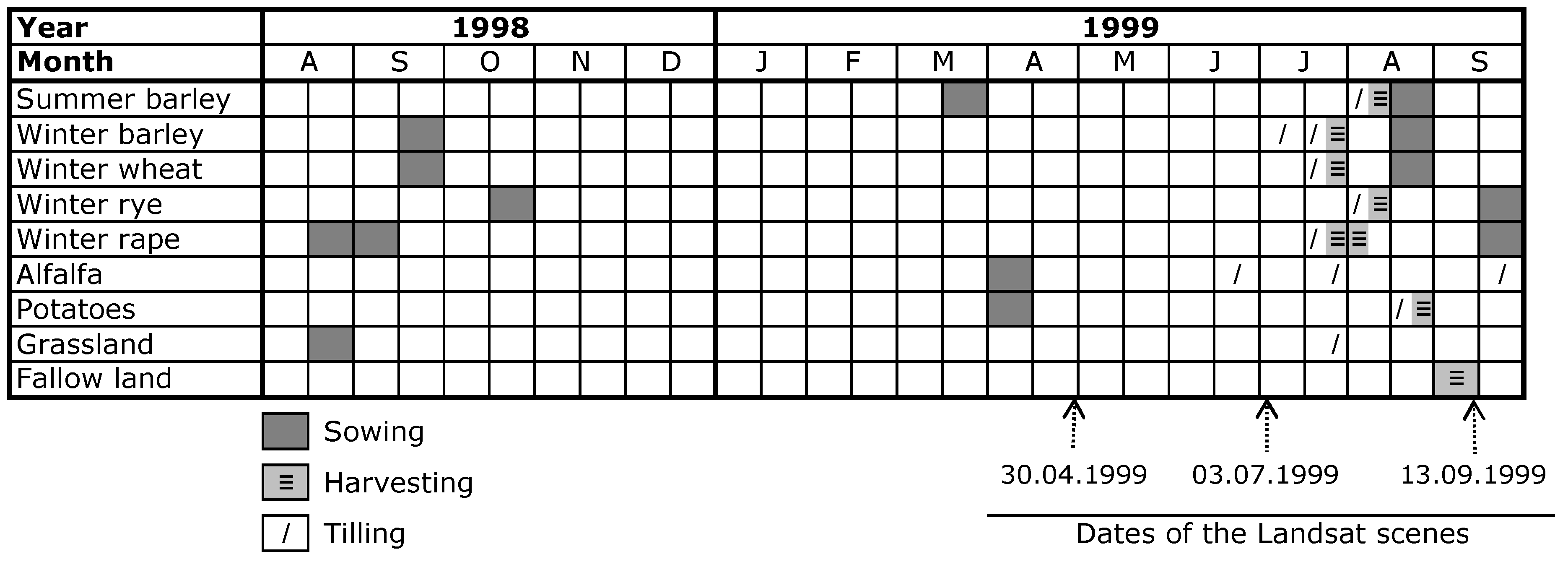
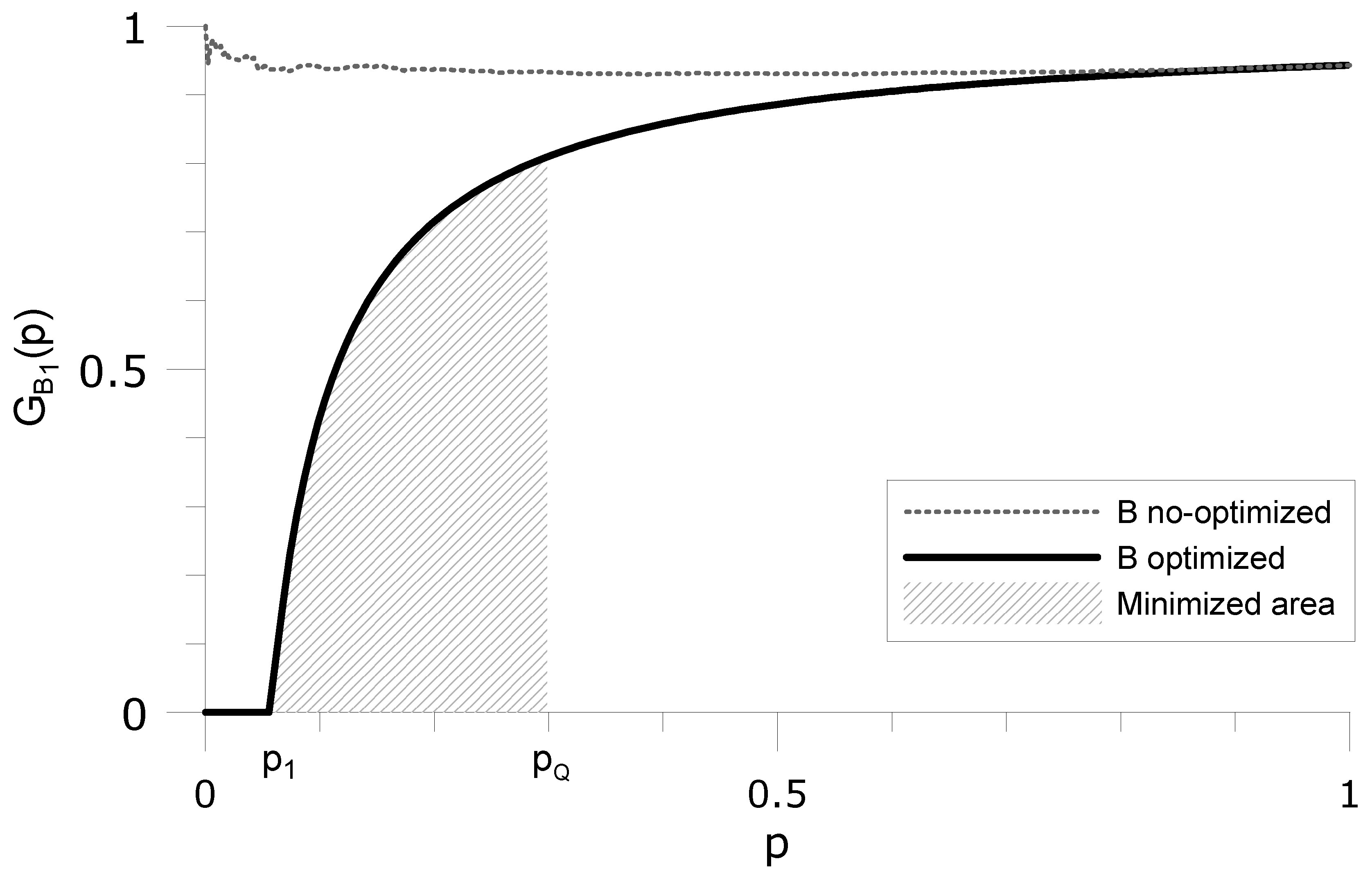
4. Results
To find the embedding spaces
, the algorithm presented in
subsection 2.3. was sequentially applied. In each optimization, the maximum limit of the integration was
(see Equation
9). The result of the optimization can be seen in
Figure 4. This graph shows that the variance function
G exhibits a completely different behavior depending on whether the distance is calculated in the original predictors’ space
or in the embedding space
. In the former, the variance of the (
p) closest neighbors remains almost constant for different values of
p, whereas in the latter an abrupt change occurs at
. This threshold represents the ratio between the number of pairs within class 1 and the total number of pairs of the boundary of the set
and has already been defined in Equation
10. Therefore, as a result of the optimization, the variance of the "outputs"
has been reduced to zero, i.e., approximately the 6% of the closest neighbors belong to class 1 in the transformed space
. This can also be visualized in
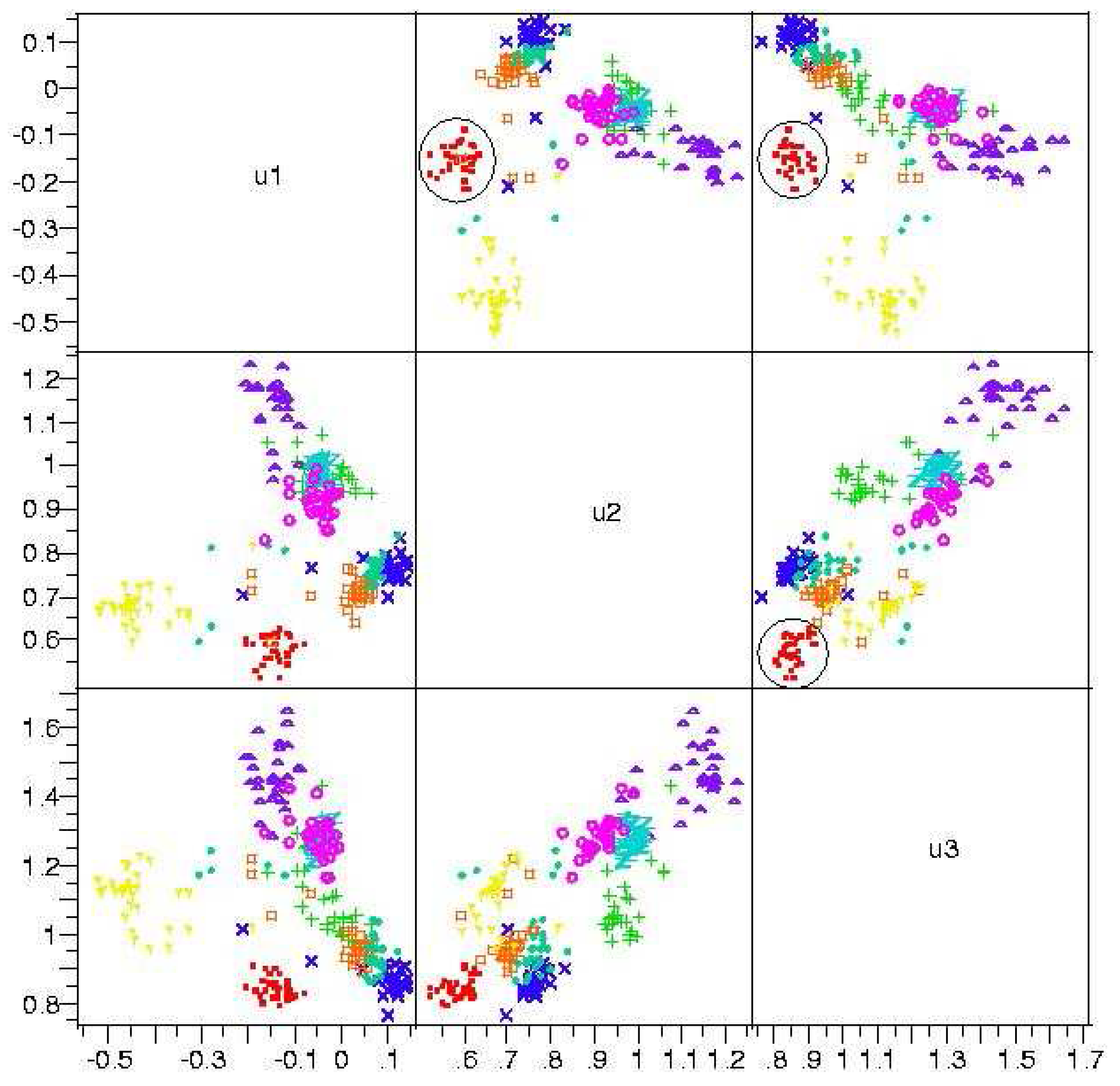
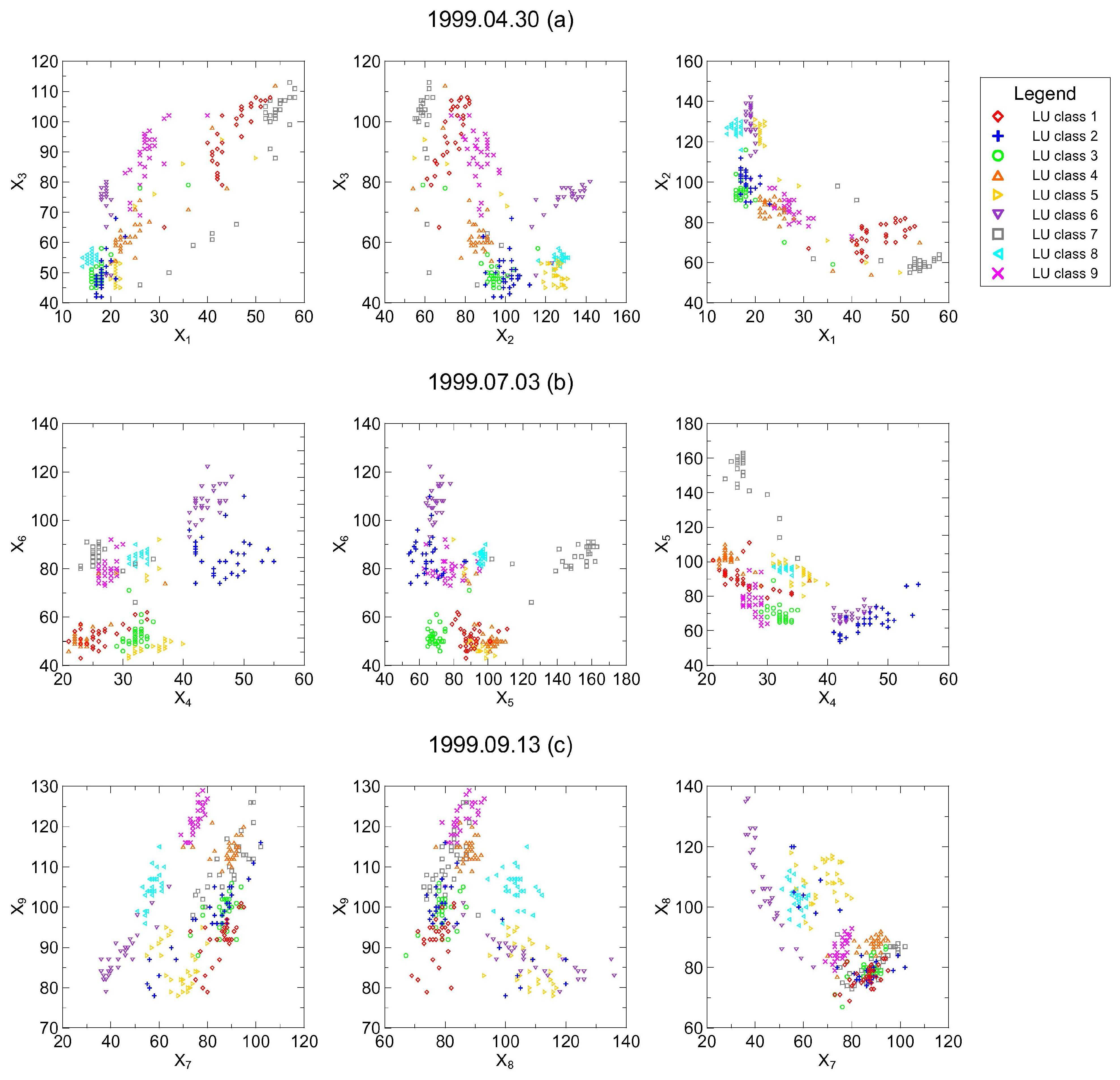
Figure 5, where it can be seen that class 1 (encircled by a continuous line) was clearly pulled apart from the rest.
Figure 4.
Effect of the optimization on the variance function . Here , i.e., the variance function of class 1 for the training set .
Figure 4.
Effect of the optimization on the variance function . Here , i.e., the variance function of class 1 for the training set .
The robustness and the reliability of the MNN method was estimated with the standard confusion matrix approach [
8]. Based on this sort of contingency table, several efficiency measures were evaluated, including: the probability of detection or producer accuracy, the user accuracy which is the complement of the false positive rate, and the overall accuracy
where
worst, and
best.
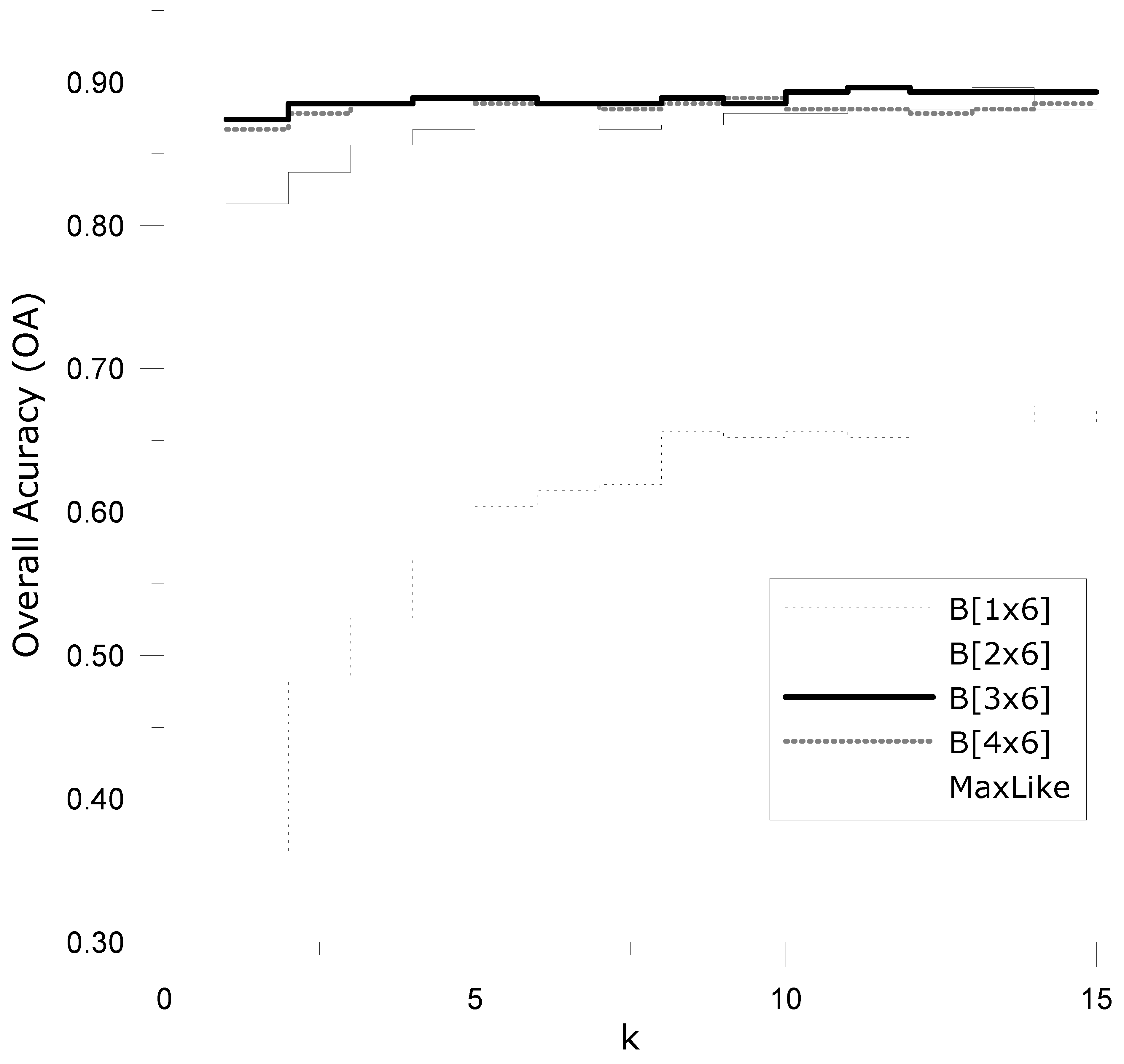
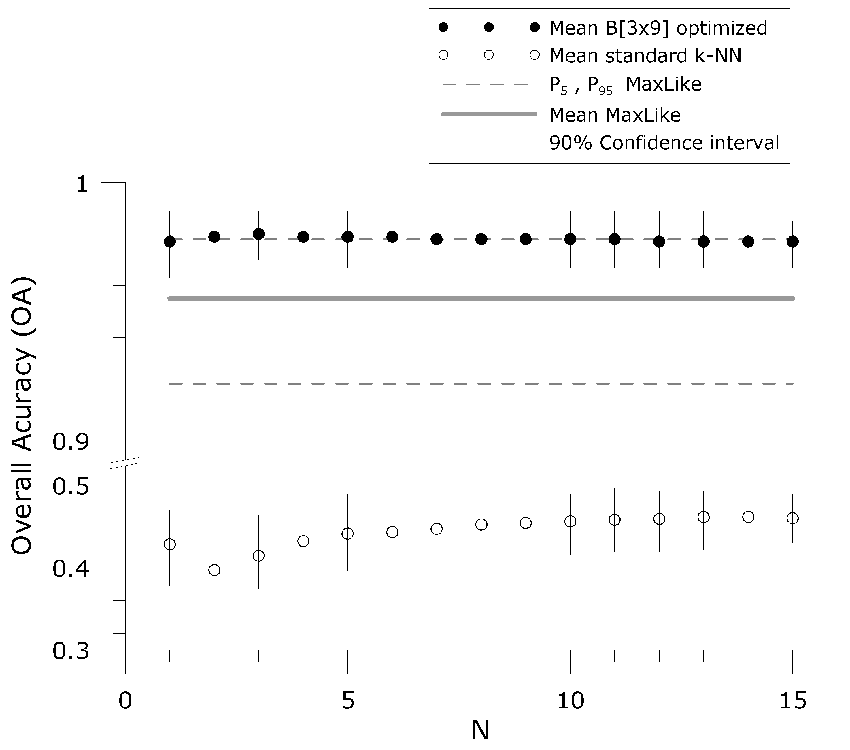
Figure 6 depicts the robustness of the proposed approach compared with both ML and the k-NN using the standard Euclidian distance in the predictors’ space (
not optimized). The 90% confidence interval of the statistic
is almost independent with respect to the number of nearest neighbors
N, which is not the case in the non-optimized case. For the estimation of empirical confidence intervals shown in
Figure 6, 100 independent training sets (
,
) were randomly sampled without replacement. The simulation results show that the average
obtained for MNN is even greater than the upper 95%-confidence limit of the results obtained with ML. The standard k-NN (without any transformation) performs poorly in all these independent samples.
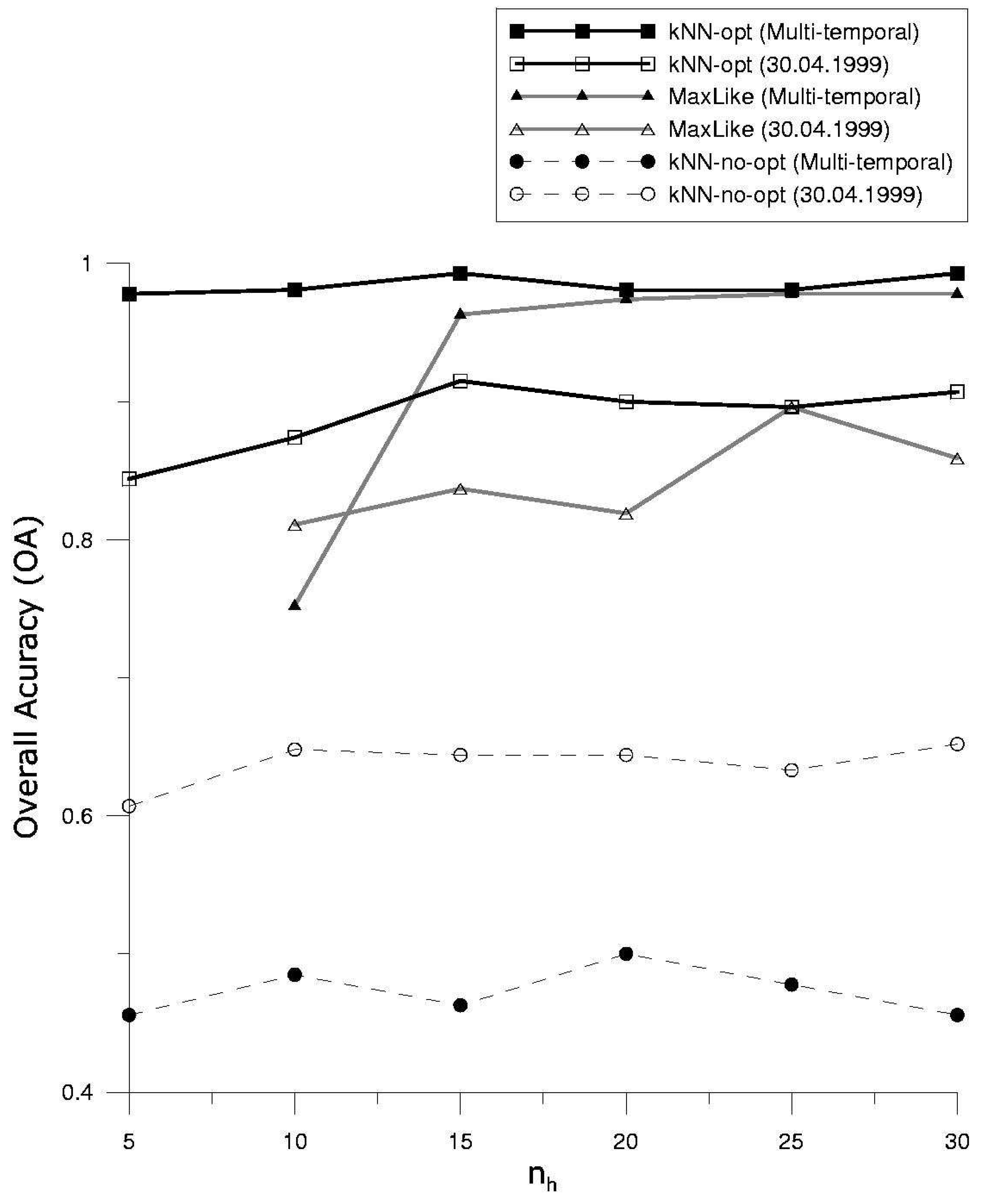
Several sensitivity analysis were carried out to determine the behavior of MNN with respect to variable composition as well to several key parameters. First, we investigated how the selection of the variables influence the efficiency of the different methods. Based on
Figure 7, it can be concluded that the multi-temporal supervised classifications provide, in general, better results than those of the mono-temporal ones. In the present case, however, k-NN with data from the 30th of April, 1999, is an exception. This indicates that k-NN might be sensitive to artifacts present (e.g., related with climate, vegetative cycle) in the data that may severely affect the efficiency of the classifier. This shortcoming has not been observed in the several hundreds of tests carried out with MNN. Another results derived from these experiments is that MNN performs much better than ML when the sample size per class (
) is small (see
Figure 7). Furthermore, influence of
on the efficiency is small. This is an advantage because it reduces the cost of data collection without jeopardizing the quality of the results.
Figure 5.
Scatterplots depicting the location of the land use classes in the embedded space . Class 1 (encircled by a continuous line) is completely isolated from the others. Sample size .
Figure 5.
Scatterplots depicting the location of the land use classes in the embedded space . Class 1 (encircled by a continuous line) is completely isolated from the others. Sample size .
Figure 6.
Graph showing the variation of the 90% confidence interval depending on the number of nearest neighbors. As reference the confidence intervals for ML and k-NN ( not optimized) are also shown.
Figure 6.
Graph showing the variation of the 90% confidence interval depending on the number of nearest neighbors. As reference the confidence intervals for ML and k-NN ( not optimized) are also shown.
The selection of the dimension of the embedding space
k plays a very important role on the efficiency of MNN as can be seen in
Figure 8. Because there are no rules for the determination of
k the trial-and-error approach was followed. This figure shows that embedding a large dimensional space into an scalar (i.e.,
) is not a good solution. As
k approaches
m, the same effect is observed, i.e. large values of
k do not perform much better than that of the
-case. It should be noted that increasing
k by one increases the number of degrees of freedom
l times. In the present case the best results were obtained for
in the mono-temporal experiment. A modification of the Mallows-CP [
35] statistic, however, was suggested in [
22] to help determine the most efficient embedding dimension, which can also be used in this context.
Based on the results of the sensitivity analysis, the final classification of the whole area of the test sites was carried out using multi-temporal data (bands 3-4-5 form the three scenes) embedded into a three dimensional space, i.e.
and using
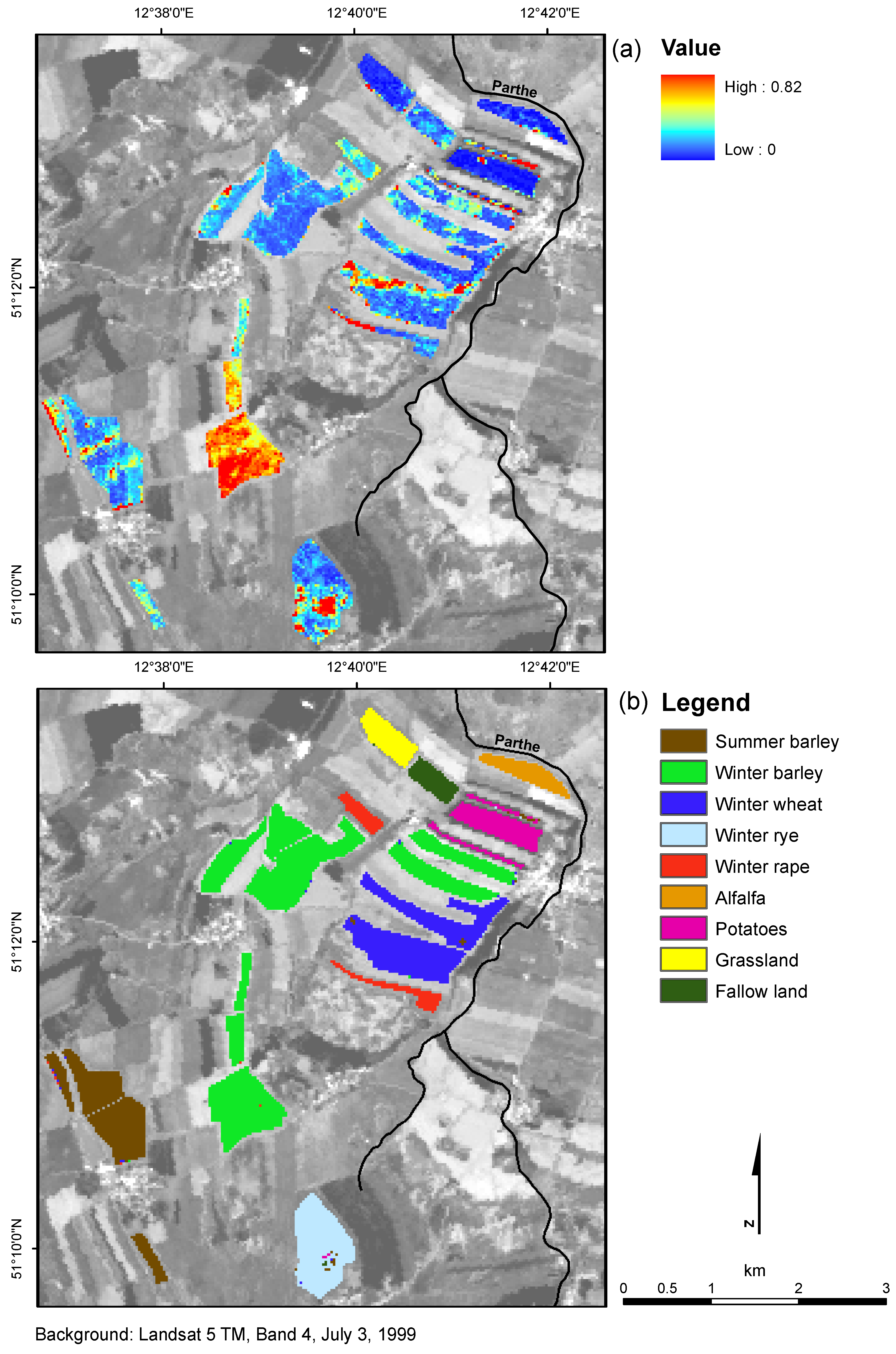
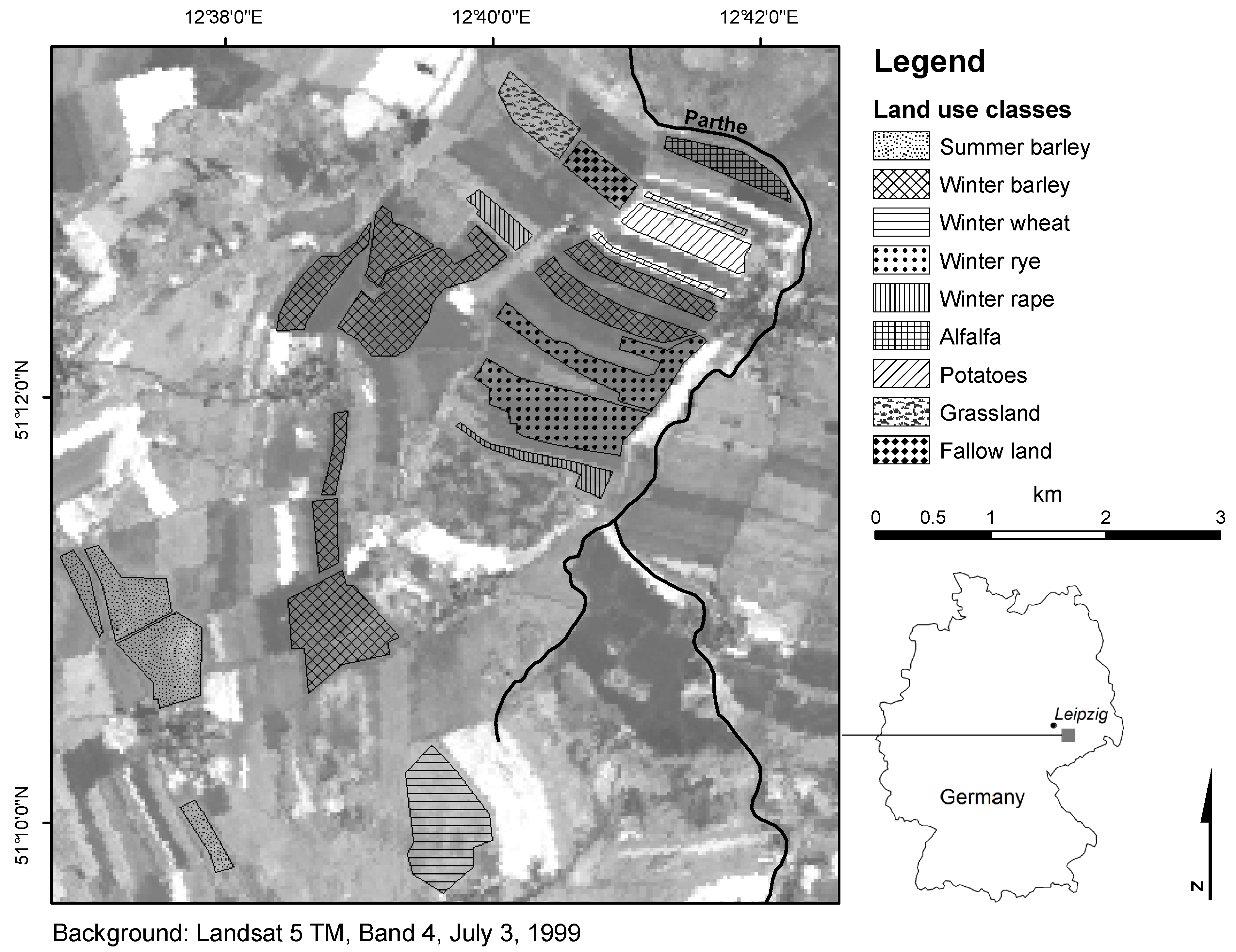
neighbors. As a result, the land cover map depicted in
Figure 9 was obtained. Additionally, the ambiguity index
proposed in Equation (
13) was estimated. With the help of this index, it is possible to determine those places where the classification is not clear (say
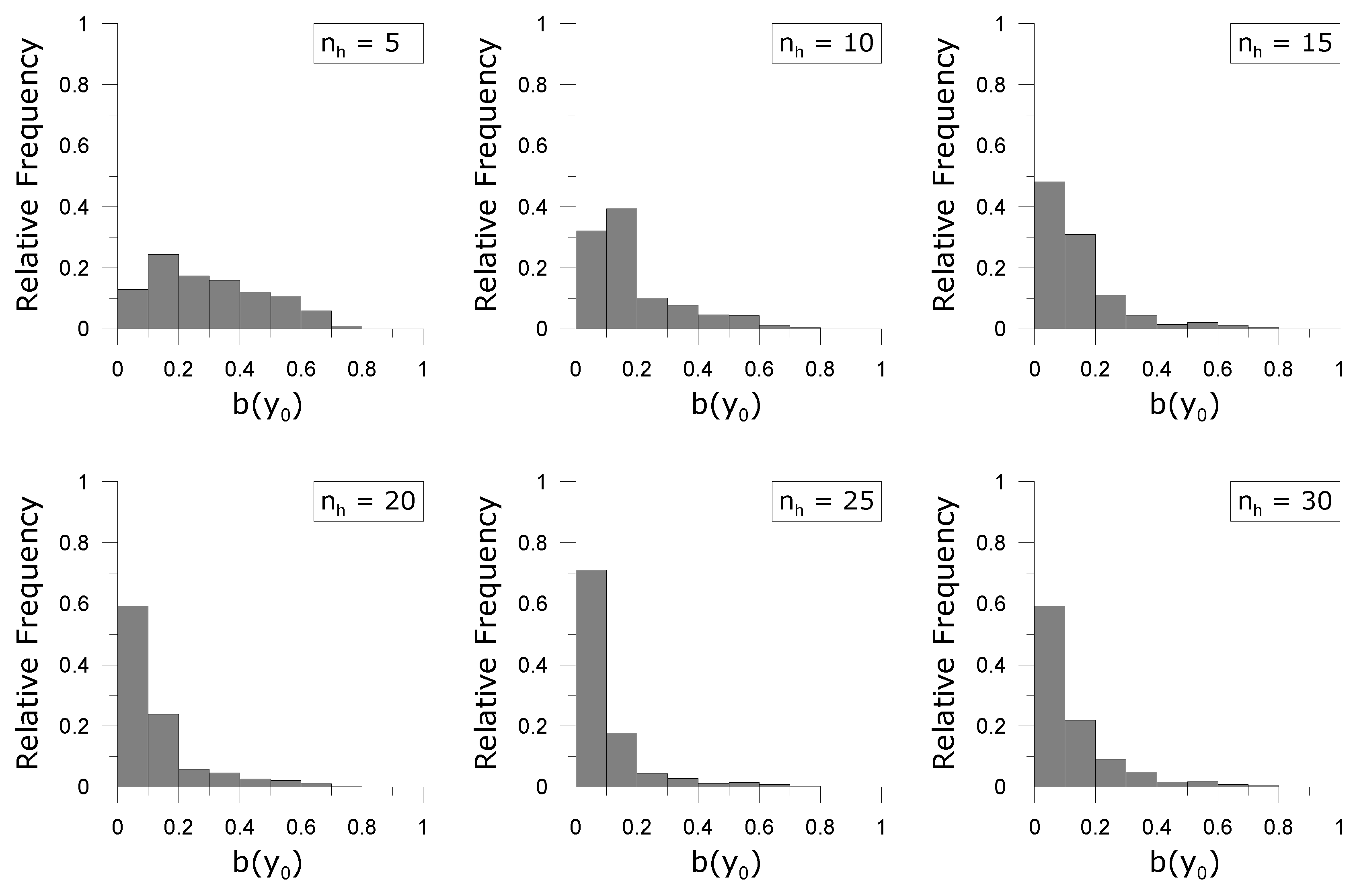
). Consequently, one should interpret the results in those areas carefully and try to determine why the classifier performs ambiguously on these areas (e.g., a very mixed class or errors in the determination in the ground truths). Furthermore, by plotting the density distribution of the ambiguity index and estimating statistics like the mean ambiguity index or the portion of pixels exceeding a given threshold, one can have a very reliable measure of the uncertainty of the classification (see
Figure 10). Taking, for example, a threshold value of
we observe that a training set consisting of only
observations for each class will have a large number of false positives, whereas with
we only obtain a very small number indicating a more reliable classification. The slight increase of the classification uncertainty between
and
suggest that large training sets might be less efficient due to possible data artifacts introduced during the sampling process. We here find an optimum sample size of
observation per class.
Figure 7.
Graph showing the influence of the sample size per class on the overall accuracy of the classification. The dimension of the transformation matrix in the mono- and multi-temporal classifications is and respectively.
Figure 7.
Graph showing the influence of the sample size per class on the overall accuracy of the classification. The dimension of the transformation matrix in the mono- and multi-temporal classifications is and respectively.
Figure 8.
Graph showing the influence of the type of transformation and the number of nearest neighbors on the overall accuracy of the classification.
Figure 8.
Graph showing the influence of the type of transformation and the number of nearest neighbors on the overall accuracy of the classification.
Figure 9.
Ambiguity index [panel (a)] and land cover map obtained with the MNN classifier using neighbors [panel (b)].
Figure 9.
Ambiguity index [panel (a)] and land cover map obtained with the MNN classifier using neighbors [panel (b)].
Figure 10.
Histograms depicting the ambiguity index as a function of the sample size of the training set . (All histograms were obtained with the MNN classifier using neighbors.)
Figure 10.
Histograms depicting the ambiguity index as a function of the sample size of the training set . (All histograms were obtained with the MNN classifier using neighbors.)
5. Summary and Conclusions
Here, we have introduced an improved k-NN technique based on a combination of a local variance reducing technique and a linear embedding of the observation space into an appropriate Euclidian space (MNN) and applied this method to a (supervised) land use and cover (LULC) classification example using mono- and multi-temporal Landsat imagery. Results show that MNN performs significantly better than both Maximum Likelihood (ML) and the standard k-NN method for all cases considered. The advantage of using multi-temporal data was also confirmed for the MNN method.
While the efficiency of the ML is dependent on a sufficient large sample size, a further strength of MNN is its small sensitivity to the cardinality of the training set leading to a more robust and cost-effective calibration of the classification problem. The formulation of an ambiguity index and its distribution provides a good measure of the uncertainty associated with a classification. Analysis of its spatial extent and characteristic will allow critical areas and LULC types within the classification process to be identified so that additional effort in ground-truth and calibration activities can be organized in a more focussed and efficient way.
Given these advantages of MNN compared with standard methods, it will be of particular interest for any of the current and future global or regional observation activities, where large areas have to be (frequently) explored under limited resources. Good examples are the Global Observation of Forest and Land Cover Dynamics (GOFC-GOLD) or the Monitoring Agriculture by Remote Sensing and Supporting Agricultural Policy (MARS-CAP) projects (among many others).
However, before becoming operational, some further aspects of the method still have to be investigated. So far, we have limited our analysis to the classification of agricultural land use types using Landsat images with a spatial resolution of 30m as presented here in this paper and to hydrologically related application considering 3 different land use classes (forest, pervious and impervious). This needs to be extended considering a broader spectrum of LULC types as well as different levels of informational aggregation. Data from different sensors and platforms need to be analyzed in order to explore the sensitivity and efficiency of our method to different spatial and spectral resolutions. However, given the results presented here and in our previous application [
23], MNN is expected to also outperform other classification methods under these conditions.
Analyzing in detail the robustness and transferability of the optimized transformation of the observation space to other geographic locations will help to keep the cost for calibration to a minimum. Also, information on the scale and temporal invariance of the transformation will be of great importance. The MNN technique might be further improved by considering non-linear transformations and/or some appropriate formulation for its variations within the observation space. While being beyond the scope of this paper, these aspects will direct our future research activities and will be presented in the near future.


