An Automated Artificial Neural Network System for Land Use/Land Cover Classification from Landsat TM Imagery

Abstract

This paper focuses on an automated ANN classification system consisting of two modules: an unsupervised Kohonen’s Self-Organizing Mapping (SOM) neural network module, and a supervised Multilayer Perceptron (MLP) neural network module using the Backpropagation (BP) training algorithm. Two training algorithms were provided for the SOM network module: the standard SOM, and a refined SOM learning algorithm which incorporated Simulated Annealing (SA). The ability of our automated ANN system to perform Land-Use/Land-Cover (LU/LC) classifications of a Landsat Thematic Mapper (TM) image was tested using a supervised MLP network, an unsupervised SOM network, and a combination of SOM with SA network. Our case study demonstrated that the ANN classification system fulfilled the tasks of network training pattern creation, network training, and network generalization. The results from the three networks were assessed via a comparison with reference data derived from the high spatial resolution Digital Colour Infrared (CIR) Digital Orthophoto Quarter Quad (DOQQ) data. The supervised MLP network obtained the most accurate classification accuracy as compared to the two unsupervised SOM networks. Additionally, the classification performance of the refined SOM network was found to be significantly better than that of the standard SOM network essentially due to the incorporation of SA. This is mainly due to the SA-assisted classification utilizing the scheduling cooling scheme. It is concluded that our automated ANN classification system can be utilized for LU/LC applications and will be particularly useful when traditional statistical classification methods are not suitable due to a statistically abnormal distribution of the input data.

1. Introduction

Multispectral classification of remotely sensed data has been widely used to generate thematic Land-Use/Land-Cover (LU/LC) inventories for a range of applications including urban planning, agricultural crop characterization, and forest ecosystem classification [1,2,3,4]. In response, a number of different classification approaches have been developed to accomplish such tasks [5,6,7,8]. Most notable have been classification approaches based on Artificial Neural Networks (ANNs) [9,10,11,12,13]. ANNs were originally designed as pattern-recognition and data analysis tools that mimic the neural storage and analytical operations of the brain. ANN approaches have a distinct advantage over statistical classification methods in that they are non-parametric and require little or no a priori knowledge of the distribution model of input data [14]. Additional superior advantages of ANNs include parallel computation, the ability to estimate the non-linear relationship between the input data and desired outputs, and fast generalization capability. Many previous studies on the classification of multispectral images have confirmed that ANNs perform better than traditional classification methods in terms of classification accuracy, such as maximum likelihood classifiers [14,15,16,17].

Based on the widely-used commercial software package ERDAS IMAGINE 9.0, we developed an automated ANN classification system to the most commonly used image classifiers such as Minimum Distance, Parallel Piped, and Maximum Likelihood in order to offer a more feasible and computationally efficient classification alternative. Our automated ANN classification system consisted of two ANN modules: 1) a single unsupervised Kohonen’s Self-Organizing Mapping (SOM) neural network module, and 2) a supervised Multi-Layer Perceptron (MLP) network module. The MLP network module is trained using the traditional back propagation (BP) training algorithm. In the SOM network module, two training algorithms were provided: 1) the standard SOM competitive learning algorithm, and 2) a modified SOM learning algorithm incorporating Simulated Annealing (SA) because it has the potential to find or approximate the global or near global optimal in a combinatorial optimization problem. The modified SOM learning algorithm with the embedded SA global searching algorithm has an advantage over the standard SOM methodology because it can utilize the scheduling cooling scheme and can resolve the local minima problem and thus improves the final classification accuracy [18,19].

This paper focuses on two primary questions:

Is the automated ANN classification system suitable for LU/LC classification applications?

Can the modified SOM-SA network perform classification more accurately than the standard SOM network?

LU/LC classifications were conducted using Landsat Thematic Mapper (TM) data and the supervised MLP network and two unsupervised SOM networks. This paper is structured as follows: Section 2 will provide a short review of MLP and SOM neural network models. Section 3 will describe the development of our automated ANN classification system and our classification procedures. Our case study is presented in Section 4, along with a comparison and evaluation of the performance of each of the classifiers based on the experimental results. Related implementation issues are also discussed. The final section presents the conclusions of the paper.

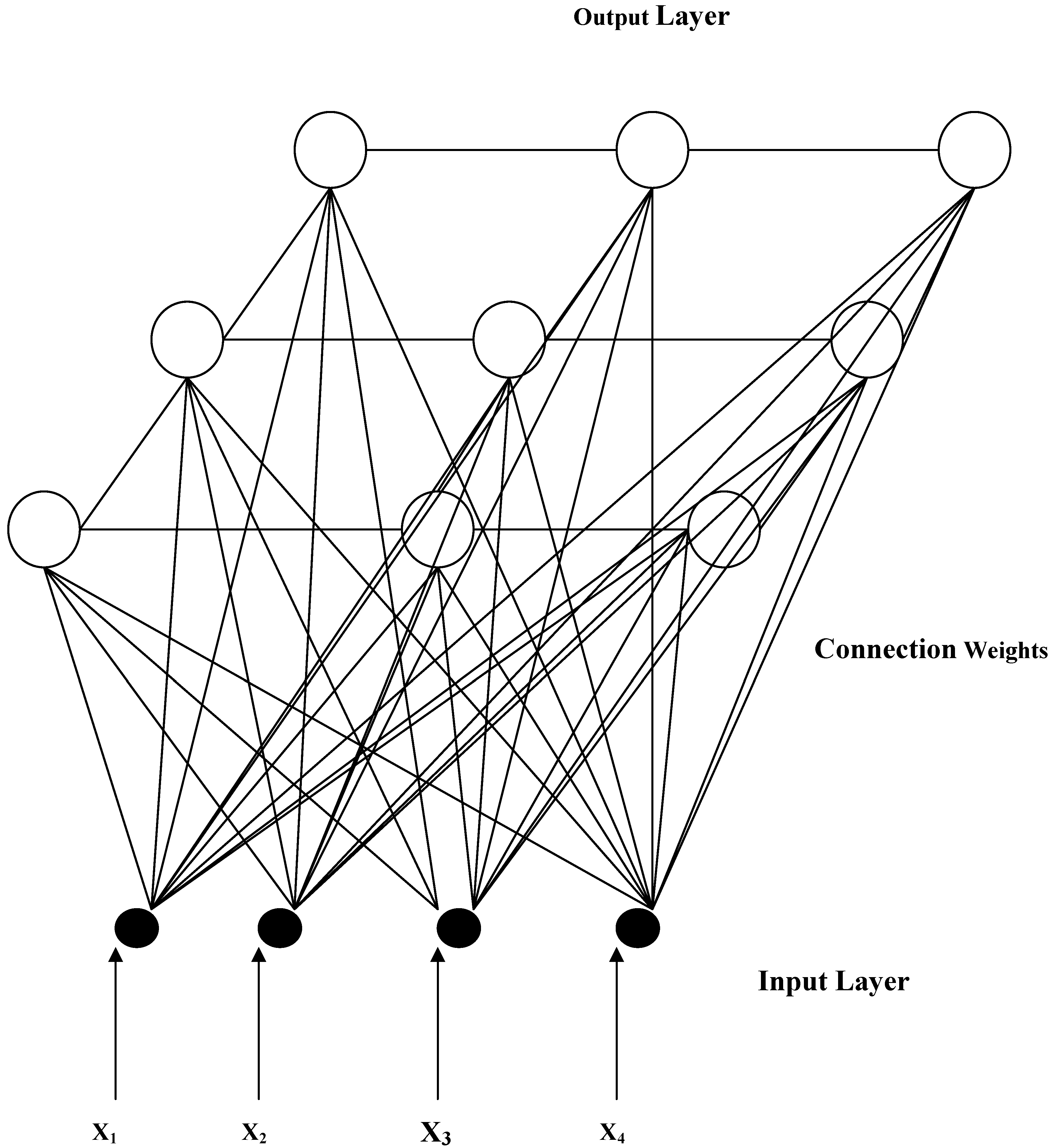
2. Neural Network Classification Approaches

While various ANN approaches have been applied to many LU/LC classification applications using remotely sensed data [14,20,21,22], the two most frequently-used neural networks are the supervised Multilayer Perceptron (MLP) [23], and the unsupervised SOM [24,25].

The MLP neural network—a supervised model that uses single or multilayer perceptrons to approximate the inherent input-out-put relationships—is the most commonly used network model for image classification in remote sensing [26,27,28]. MLP networks are typically trained with the supervised backpropagation (BP) algorithm [23] and consist of one input layer, one or more hidden layers, and one output layer (Figure 1).

In the traditional BP algorithm, the generalized delta rule used to update the weights is usually very slow and unstable. Both [29] and [30] found that an enhanced neural network can be achieved by incorporating a momentum term (the past increment to the weight) to speed up and stabilize the BP learning. Although there are many examples of successful MLP applications [11,17,26,27,28,31,32], it is widely recognized that MLPs are sensitive to many operational factors including the size and quality of the training data set, network architecture, training parameters, and over-fitting problems. These factors are application-dependent and best addressed on a case-by-case basis. Thus, the operational issues will be discussed in concert with the case study in Section 4.

Figure 1. The structure of three-layer MLP neural network with 4 input nodes, 10 hidden nodes, and 5 output nodes. Each hidden layer is directly connected to each component of the input layer and also to each of the components in the output layer.

Figure 1. The structure of three-layer MLP neural network with 4 input nodes, 10 hidden nodes, and 5 output nodes. Each hidden layer is directly connected to each component of the input layer and also to each of the components in the output layer.

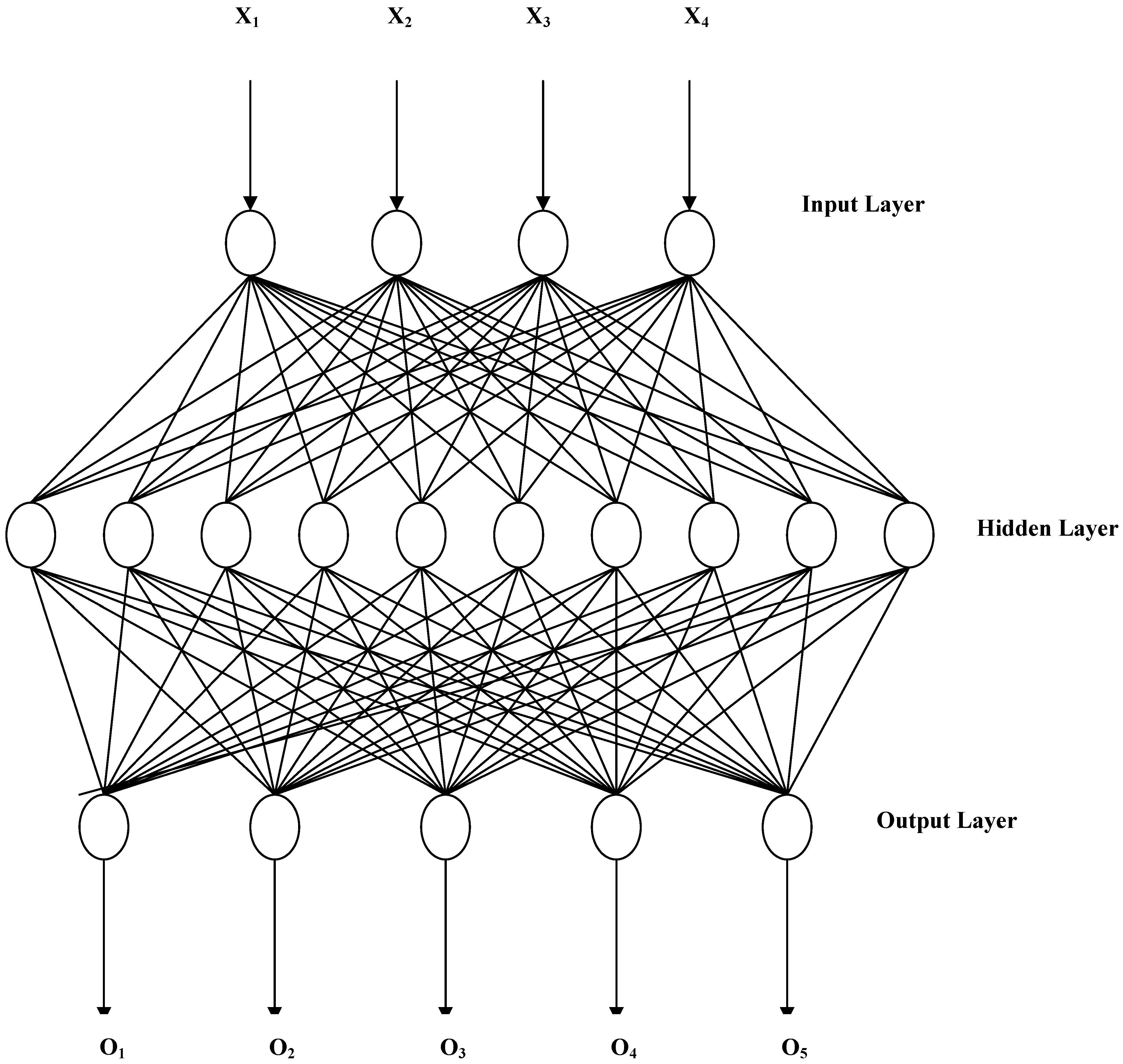
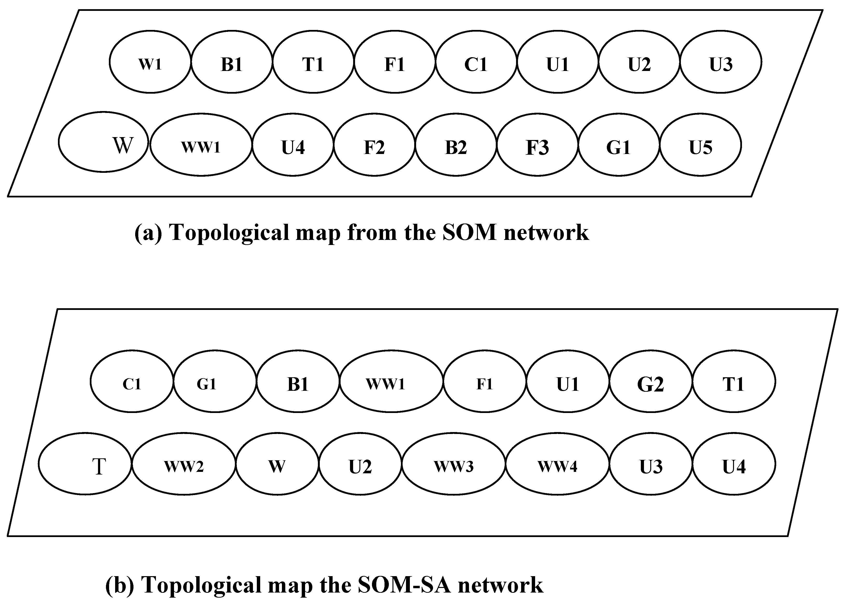
2.1. Kohonen’s Self-Organizing Mapping (SOM) Neural Network

Developed as an unsupervised clustering ANN, Kohonen’s Self-Organizing Mapping (SOM) network [25] creates a one- or two-dimensional map of relationships among input data patterns (Figure 2).

Figure 2. The structure of Kohonen’s Self-Organization Mapping neural network.

Figure 2. The structure of Kohonen’s Self-Organization Mapping neural network.

SOM networks have been found to be capable of analyzing complex multivariate data from natural systems [10]. The standard SOM algorithm is summarized by [33,34]. During training, the SOM has an input layer that can accept multiple inputs that are passed to an output or competitive layer consisting of one or two dimensions. A node in the competitive layer with the weight vector closest to this input vector in terms of Euclidean distance is called the “winning” node. Only this winning node and the nodes in its neighbourhood update their weight vectors during the training procedure. This spatial neighbourhood property makes the SOM network different from other competitive networks [30] as it has the ability to preserve the topological relationships in the original input data, by which the clusters with similar spectral signatures in image classification are assigned to the neighbouring nodes in the competitive layer [35].

The SOM neural network is particularly ideal for classification problems where class labels for training patterns are impossible or very expensive to obtain (e.g., heterogeneous landscape conditions). SOM also has operational advantages over supervised methods in terms of reduced interaction time by the analyst; however, it offers less control over the resulting classes [36].

K-means clustering algorithms produce similar classification results as SOM neural networks because they have a similar objective—to minimize the distances between the input patterns and the assigned clusters centres via a gradient descent-based searching process. K-means type algorithms are known to produce good results only if the clusters are well-separated in the feature space, and hyperspherical in shape when Euclidean distance is used. However, in a complex problem that cannot be solved by a simple convex cost function, the local minima problem is inevitable.

Alternatively, Simulated Annealing (SA) was developed on the basis of an analogy between the physical annealing process of solids and the large combinatorial optimization problems [37,38,39,40]. SA was proven to have great potential to find or approximate the global or near-global optimal in a combinatorial optimization problem [41]. The premise of SA is to incorporate some randomness in the assignments of cluster labels to pixels in the clustering procedure, thus reducing the limitation of local minima. As a result, using the SA-based approach to classification has the potential to improve the accuracy for land cover classification.

In this investigation, the standard SOM learning algorithm was modified by incorporating SA global searching procedures. The modified SOM-SA uses a cooling schedule required by most SA-related applications. This combination of SOM and SA therefore becomes an interesting contribution to the classification of digital remotely-sensed data for land use and land cover application. For the SOM-SA training, a control parameter denoted as the temperature T was introduced. The SOM-SA procedure is as follows:

Start with a high temperature T that decreases gradually and an arbitrary initial assignment of each training pattern to an arbitrary output node.

An input pattern X_i is randomly selected and presented to the SOM-SA network. The input pattern presented to this network is selected based on a parameter called generation probability.

For each randomly selected input pattern, X_i, reassign it to an output node n that is different from its previous assigned output node m.

Compute the Euclidean distances between the input patterns and each output node.

Instead of simply choosing the output node with the closest weight vector in the standard SOM learning algorithm, the winning node is determined either with a distance decrease, or with a distance increase according to a positive probability of the temperature at this state.

Repeat steps 2 to 5 until a certain number of iterations are reached at this temperature.

Decrease the temperature T in a given schedule.

Go to step 2 until the temperature T approaches zero.

The SOM-SA learning algorithm is less computationally efficient than the standard SOM learning algorithm, but has the advantage of more frequently escaping the local minima limitations as compared to the standard SOM and therefore is expected to improve classification performance.

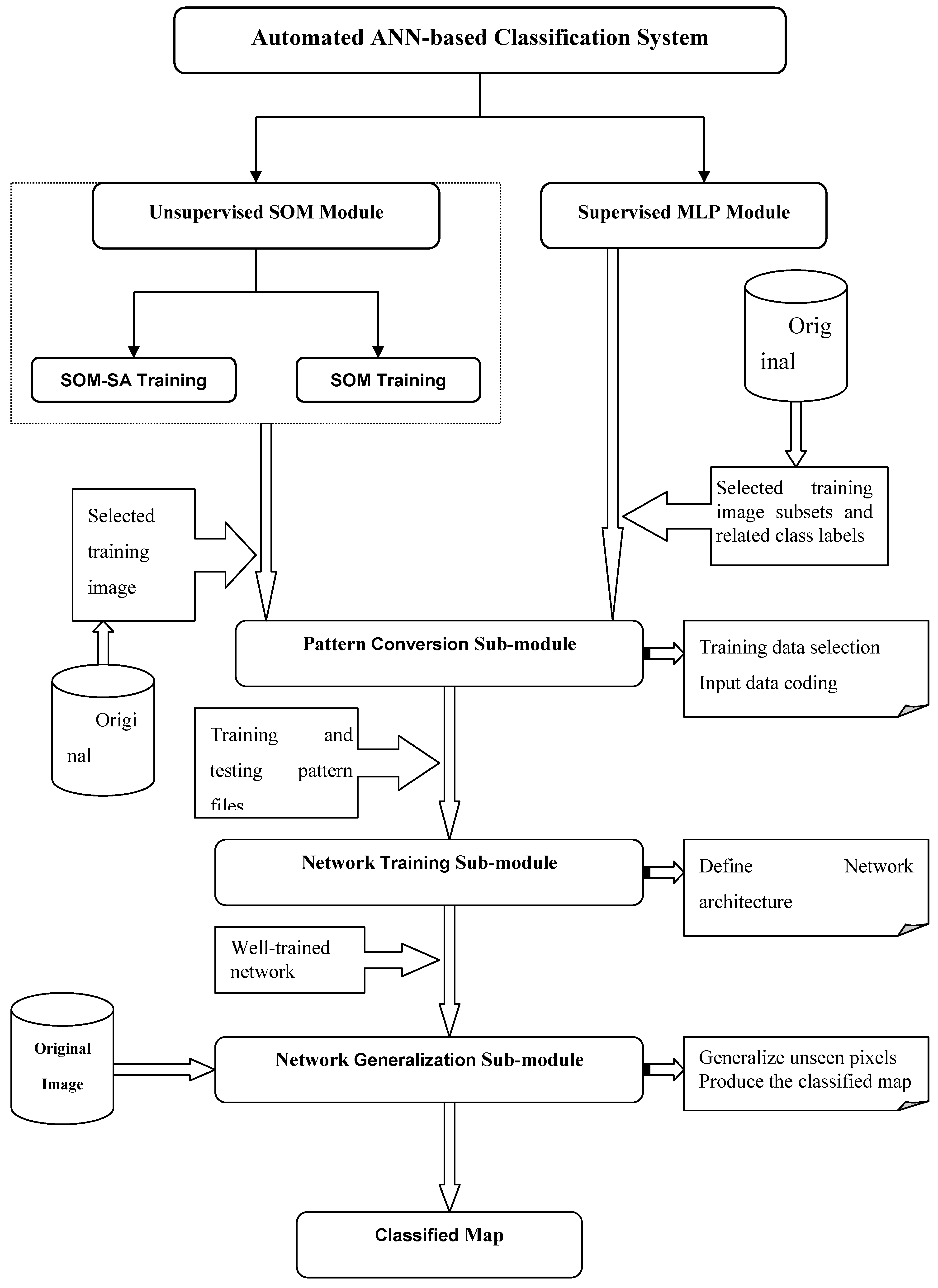
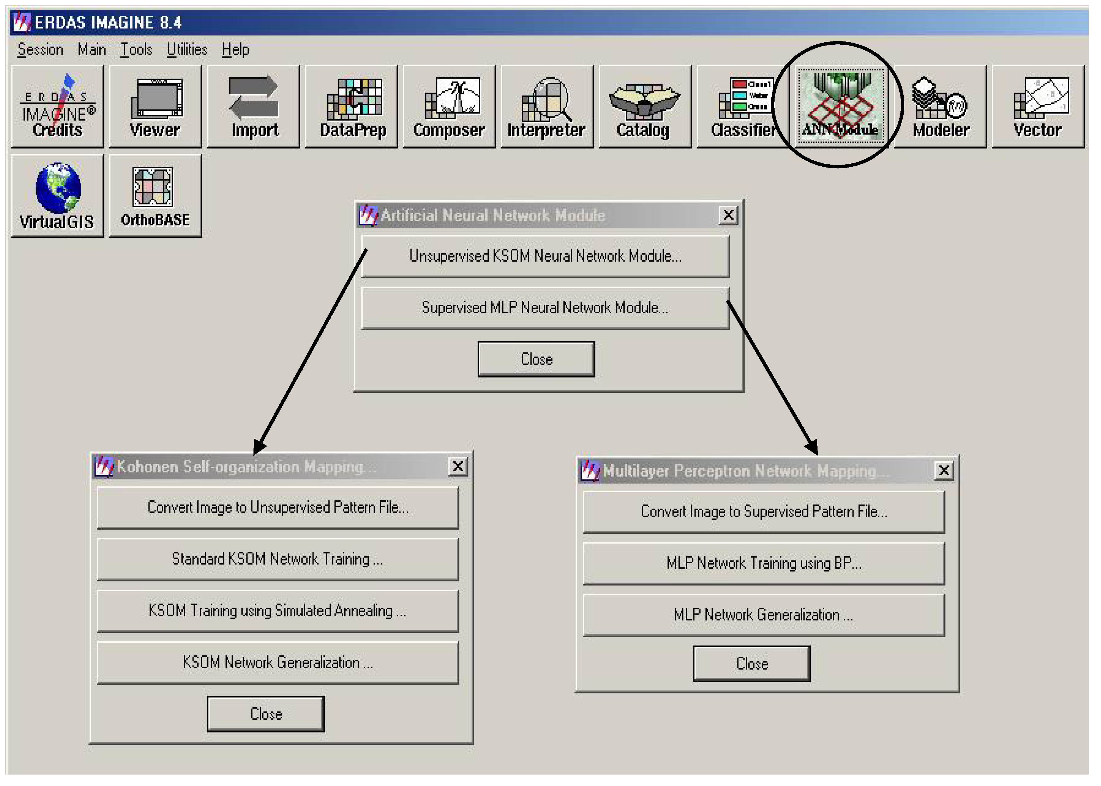
3. Development of an Automated ANN Classification System

ANN approaches have been widely used for image classification in remote sensing since the 1990s [24,27,31,32,42,43,44]. Our automated ANN classification system was built within the working environment provided by the commercial remote sensing software, ERDAS IMAGINE 9.0 [45].

The automated system consists of three classification modules: 1) a SOM module based on unsupervised SOM neural networks, 2) a modified SOM module to utilize the SA allowing a scheduling cooling scheme, and 3) a MLP module based on supervised MLP neural networks.

Each module in the ANN system is composed of several sub-modules: pattern conversion, network training, and the network generalization sub-module. The ANN-based classification system and functions of each sub-module are summarized in a working flowchart (Figure 3). Several steps take into account the unsupervised SOM and the supervised MLP classification results in determining the pattern conversion sub-module for the desired output data before creating the network training sub-module that in turn defines the training parameters for a well-trained network. These results are then applied to the unseen pixels of the original image to produce the classified map.

The pattern conversion sub-module performs the following functions:

1) sampling a certain number of training and testing patterns from a number of selected image subsets;

2) scaling the input pattern into the network operational interval; and

3) generating training or testing pattern files.

In the pattern conversion sub-module of the supervised MLP network, the corresponding class label must be provided for each pattern. Network training sub-modules provide the graphical user interfaces to allow the user to interactively define the architecture and parameters needed and to perform the training once all the parameters are set. In the SOM module, two training sub-modules are provided: the standard SOM and the SOM-SA training sub-module. In the MLP module, the BP training sub-module is used. During a network training trial using each of the training sub-modules, an error file is generated to record the training MSEs to assist in monitoring the training behaviour and selecting the appropriate network and parameters. After training is completed, network generalization sub-modules are implemented to generalize the entire image using the trained network and to produce the classified map.

The primary graphical interfaces of the ANN system (Figure 4), were built using ERDAS IMAGINE EML [45]. The ANN classification algorithms were implemented using C/C++ and the ERDAS IMAGINE Toolkit [45].

Figure 3. Flowchart of the ANN-based classification system.

Figure 3. Flowchart of the ANN-based classification system.

Figure 4. Main interface of the ANN system.

Figure 4. Main interface of the ANN system.

4. Case Study: Neural Network Classification

A Landsat TM image was used to test of the suitability of our automated ANN system in performing LU/LC classifications using the supervised MLP network and the two SOM networks.

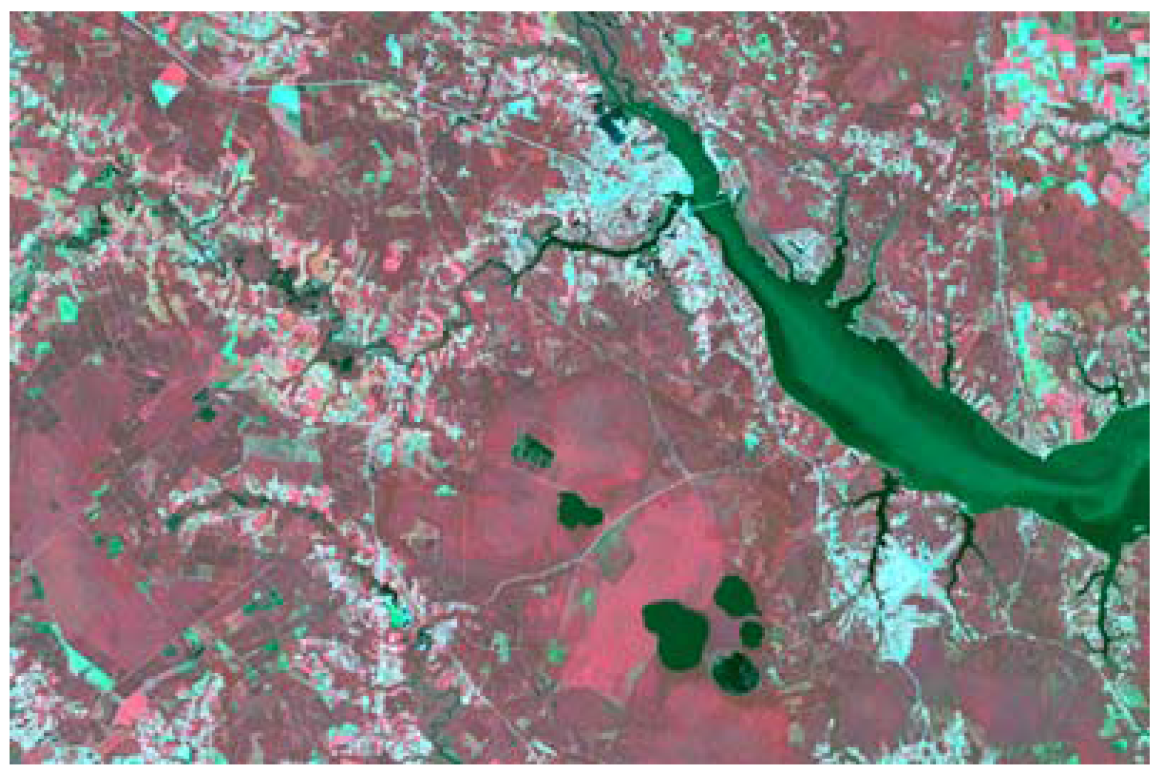
4.1. Study Area and Classification Scheme

The lower Neuse River Basin region of North Carolina—including Craven, Jones, Pamlico, and Onslow counties—was used as a study area due to the variety of urban, agricultural, and hydrologic thematic features in the coastal plain. The dominant classes include: forest, agricultural lands, and open water, and there are large areas of woody wetlands and transitional lands. A September 1999 Landsat TM image (Figure 5), was used to perform the classification. By visually interpreting this image with the high spatial resolution Digital Color Infrared (CIR) Digital Orthophoto Quarter Quad (DOQQ) data of the study area (acquired between January and March 1998), the classification scheme (Table 1) was determined using the LU/LC classification scheme proposed by [46]. Eight major categories were defined. Six TM bands, with a spatial resolution of 30 m were used for the classification. The thermal band was excluded because its spatial resolution (60 m) would require additional pre-processing work.

Figure 5. The standard false color display of the acquired Landsat TM image.

Figure 5. The standard false color display of the acquired Landsat TM image.

Table 1. Classification scheme and category definition.

Class Number	Class Name	Class Definition
1	Urban	Commercial/Industrial/Residential/transportation
2	Forest	Natural Forested Upland including evergreen, deciduous, and mixed forests
3	Planted crop field	Planted crop fields for the production of crops
4	Grass/pasture	Vegetation planted in developed settings for recreation, erosion control, or aesthetic purposes, or hay crops or pasture
5	Bare/fallow area	Bare construction sites, rock, sand, or fallow agricultural land
6	Transitional area	Areas dynamically changing from one land cover to another
7	Woody wetland	Areas of forested or shrubland vegetation where soil or substrate is periodically saturated with or covered with water
8	Water	All areas of open water

Table 1. Classification scheme and category definition.

Class Number	Class Name	Class Definition
1	Urban	Commercial/Industrial/Residential/transportation
2	Forest	Natural Forested Upland including evergreen, deciduous, and mixed forests
3	Planted crop field	Planted crop fields for the production of crops
4	Grass/pasture	Vegetation planted in developed settings for recreation, erosion control, or aesthetic purposes, or hay crops or pasture
5	Bare/fallow area	Bare construction sites, rock, sand, or fallow agricultural land
6	Transitional area	Areas dynamically changing from one land cover to another
7	Woody wetland	Areas of forested or shrubland vegetation where soil or substrate is periodically saturated with or covered with water
8	Water	All areas of open water

4.2. Operational Issues in Neural Network Classification

Although previous studies have proven neural network approaches to be powerful, the performance of the ANN classifiers is sensitive to several factors including: 1) the quality and size of the training data sets; 2) the complexity of the network architecture; and 3) controlling parameters such as learning rate [16,43,44].

4.2.1. Quality and size of training data sets

The training data set should provide as complete a representative description of each land category as possible, thus the size of the set should increase considerably along with increases in the spectral variability of desired classes, the number of associated weights, and the desired classification accuracy [30,47] points out that incorporation of some boundary patterns from each class is particularly useful in achieving satisfactory classification accuracy. A network trained with boundary patterns may have lower training accuracy, but can have better generalizing performance than a network trained with homogeneous patterns.

4.2.2. Network architecture complexity

In a typical MLP neural network, the number of input and output nodes are usually determined by the specific application (i.e., the number of input nodes equals the input dimension and the number of output nodes equals the number of desired LU/LC categories). Single hidden layer networks are found to be sufficient for most classification problems [26,27,48]. Thus the remaining problem is to determine the number of hidden nodes in the single hidden layer. Networks with varying numbers of hidden nodes, (e.g., the same, twice, or three times the number of input nodes or output nodes), are determined through experimentation. The network architecture with the best performance is selected. In the SOM network, the number of the input nodes equals the input dimensions. Similarly, the number of the SOM output nodes may not always match the number of the desired land categories. The optimal number of the output nodes in the SOM network indicates the number of separable spectral clusters and is closely related to the geometrical characteristics of the input data

4.2.2.1. Network input/output coding

Using the ERDAS IMAGINE 9.0 platform, the input coding is conducted by the pattern conversion sub-module, which automatically scales each pattern into a vector within the range while sampling training or testing patterns from a number of image subsets. The scaled input vectors and the coded desired output unit vector (supervised case) are stored in pattern files, which are presented to network training. Most neural network algorithms are designed to deal with continuous data ranging from 0 to 1.0. Since most spectral band value ranges from 0 to 255, each input data is scaled by 255 before it is presented to the network. The inputs are also associated weights, activation function, and the bias. In the pattern conversion sub-module of the MLP classification module, the desired class label of each input pattern is coded as a unit vector with the same size as the number of classes, in which only the element with the class label is equal to 1 and all other elements are assigned to 0. The scaled input vectors and the coded desired output unit vector (supervised case) are stored in pattern files, which are presented for network training. Once the training is completed, the network generalization sub-module performs the final classification of the entire image by assigning each input pixel to the class of the output node with the highest output value or closest weight vector.

4.2.3. Training parameters and learning rate

The number of training parameters varies with the type of network and algorithm used. In our investigation, the required parameters of the MLP network included: 1) initial learning rate, 2) final learning rate, 3) the momentum rate, and 4) the number of training epochs. The learning rate must be kept small enough in order to keep the network training stable. However, the computational cost of using a very small learning rate is high. Thus, in practice one usually starts with a slightly larger learning rate to run the training faster at the early stage of training, gradually lowering the learning rate to stabilize the training. The momentum rate should also be chosen via experimentation. The number of iterations must be large enough to gain sufficient knowledge of class membership from the training data set, but not too large to have the training data over-trained. In the MLP network, we used epoch training as it is more efficient stable than pixel-by-pixel training [30]. As such, the weight adjustment from each input pixel is computed and stored without changing the weights. After the entire training set passes through the network, the average weight adjustment is used to update the weight.

Standard SOM network training requires the definition of the following parameters: 1) the initial learning rate, 2) the final learning rate, 3) the initial neighbourhood radius, 4) the neighbourhood decrement interval, and 5) the number of training iterations. The selection of learning rates and the number of training iterations is similar to that in MLP network. The initial neighbourhood radius is usually set equal to the larger size of row or column and decreases after a certain number of iterations. The determination of the initial neighbourhood radius and the neighbourhood decreasing factor is crucial for SOM networks to achieve a topology-preserving map from the input space to the discrete output. In addition to these standard SOM training parameters, SOM-SA training requires a cooling schedule as follows: 1) the initial value of the control temperature T, 2) the decrement factor for decreasing T, 3) the final value of T, 4) the number of iterations at each temperature value, and 5) a generalization probability to control which pixel in the training set is selected to train the network. Several guidelines for selecting these SA-related parameters were developed by [56]. An optimal selection of parameter combinations is critical to obtaining good classification accuracy.

Over-fitting is a situation that arises when the neural network classifier is over-trained. This problem can considerably decrease generalization accuracy when some land classes are not properly represented in training data sets. One of the most effective methods to avoid over-fitting is to use a cross-validation approach to stop the training at an appropriate time [49,50]. Basically, two data sets should be collected: one for training the network and the other for testing it. During network training, only the training data set is used to train the network and update the weights. However, the classification performances with both testing and training data are computed and monitored during the process. If training error keeps decreasing, while testing error continuously increases, the training will be terminated. Via the cross-validation approach, the training can be stopped before the over-fitting occurs [27]. Ultimately, the cross-validation approach can provide clues as to whether the collected training data sets completely represent land cover classes. Consequently, cross-validation was used as the default training method.

4.3. Neural Network Classification and Discussions

For each class, multiple image subsets were first selected from the TM image using ERDAS IMAGINE tools. Our goal was to collect image subsets from homogeneous and heterogeneous areas. The number of the image subsets for each land category varied because of the spectral variability within that category. Categories with high within-class spectral variability, such as urban and crop lands, were assigned more image subsets than others. The selected image subsets were processed using the pattern conversion sub-modules in the ANN classification system. By using this sub-module, a certain number of training and testing patterns per class were extracted from the image subsets, coded, and saved into training and testing pattern files. In MLP classification, the corresponding class label related to each sampled pattern was provided. In this application, a total of 3360 training pixels and 360 testing pixels were chosen, composed of 420 training and 45 testing pixels for each of the eight classes. During the network training, only the 3360 training patterns were used to train the network. After each iteration, the MSEs of the training and testing sets were calculated and recorded into an error file which was used to monitor the training behaviors and assist in selecting optimal network architecture and training parameters.

In the MLP classification, we used the three-layer perceptron network, consisting of six input nodes and eight output nodes. We ran a number of MLP experiments using different hidden nodes and training parameters. After each iteration, an error file was generated to record the training and testing errors. Based on these error files, the optimal network architecture and training parameters was determined. In this case, the optimal MLP network architecture was found to be a single layer network with 15 hidden nodes. The best MLP training was obtained when the parameters were set as: 1) training epochs (150,000), 2) initial learning rate (1.5), 3) final learning rate (0.05), and 4) momentum (0.08). The well-trained MLP network was input into the network generalization sub-module, and then used to classify the TM image into a map with eight LU/LC classes shown in Figure 6(a). The learning curve of the mean squared errors vs. training epochs for both training and testing sets indicated a good generalization of the trained MLP network. The cross-validation training, described earlier, method proved effective in this application in terms of avoiding over-fitting.

Figure 6. Classified maps of the three network classifiers.

Figure 6. Classified maps of the three network classifiers.

The optimal SOM network training used 16 output nodes that were arranged as two rows and eight columns. The parameters in the optimal SOM training were set as below: 1) training iterations (5000), 2) initial learning rate (0.2), 3) final learning rate (0.005), 4) initial neighbourhood size (8), and 5) the neighbourhood decrement interval iterations (400). The optimal SOM-SA training was obtained using the same architecture as the SOM network. The parameters were set as below: 1) initial T (1.0), 2) final T (0.01), 3) decrement factor of T (0.95), 4) generation probability (0.80), 5) iterations at each T (50), 6) initial learning rate (0.8), 7) decrement factor of learning rate (0.95), 8) initial neighbourhood size (8), and 9) neighbourhood decrement factor (0.75). Using the two SOM-based networks, instead of the eight classes we expected, resulted in 16 spectral clusters. We manually interpreted the 16 clusters and matched them with one of the eight classes. The two feature maps from the SOM and SOM-SA networks (see Figure 8(a-b)) were created to reflect the information class membership of each spectral cluster in this classification application. The resulting classified maps with eight classes from the SOM and SOM-SA networks are shown in Figure 6(b) and Figure 6(c), respectively.

The SOM and SOM-SA networks have topological preservation capability such that pixels with similar spectral values are assigned to the neighbouring classes, and nodes in the competitive layer with similar spectral signatures are located as near neighbours [35]. Our observation of these two feature maps (see Figures 7(a-b)) verified this phenomenon. Furthermore, by analyzing the relative location of each spectral cluster and its represented information class, we obtained some knowledge of the inherent spectral relationship between classes such as the within-class and between-class spectral variability. From Figures 7(a-b), we observed that the urban class consisted of four spectral clusters, three of which were within the close neighbourhood and one of which was farther away, indicating its widely scattered within-class variability.

Figure 7. Topological maps from the SOM and SOM-SA networks where U: Urban, F: Forest, C: Crop field, G: Grassland, B: Bare soil, T: Transitional area, WW: Woody wetland, W: Water.

Figure 7. Topological maps from the SOM and SOM-SA networks where U: Urban, F: Forest, C: Crop field, G: Grassland, B: Bare soil, T: Transitional area, WW: Woody wetland, W: Water.

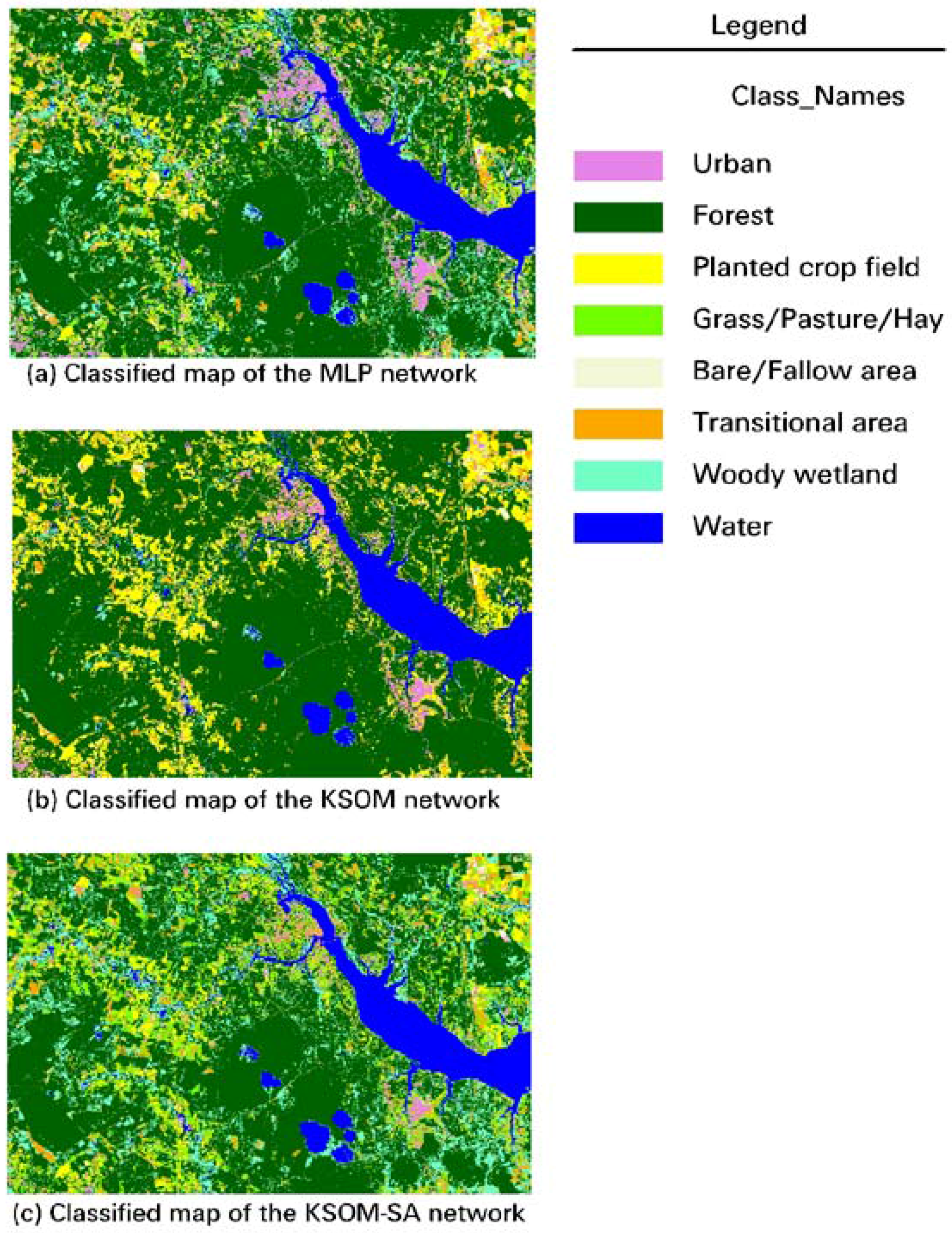
4.3.1. Accuracy assessment

To evaluate the three resultant classified maps, we assessed the classification accuracy based on a pixel-by-pixel comparison. Using a stratified sampling method, 60 pixels per class were randomly selected from the MLP classified map and a total of 480 pixels were used for the accuracy assessments of the three network classifiers. That is, the sample size for the accuracy assessment was 60 samples per land use/land cover category. While using the data collected by field visitation as reference data is always preferred, we feel that the level of details observed on the very high resolution one-meter digital multispectral data produced no confusion between the classes of interest in this study and therefore judged appropriate to be used as reference data. To this effect, the three error matrices for the three classifications were generated by visually and carefully interpreting the one-meter CIR DOQQ for each sample site and the corresponding TM imagery for each of the 480 pixels as shown in Table 2 to Table 4. This type of very high resolution multispectral imagery has often used as reference data where field data was not available [53]. An error matrix provides an appropriate beginning for many techniques of multivariate statistical analysis [51]. One measure used in accuracy assessment is called KAPPA [52]. KAPPA is designed to deflate the amount of agreement by the amount, which would be expected by chance. It can be interpreted as a “proportionate reduction in error”, the proportion that the results improve upon a model of statistical independence (the cross-product term in the above equation).

Table 2. Error matrix on the classified map from the MLP network.

		Reference Data
Classified Image		1	2	3	4	5	6	7	8	Classified Totals	Users’ Accuracy
	1	46	1	1	1	11				60	76.7%
	2		60							60	100.0%
	3		2	52	6					60	86.7%
	4		2	4	53	1				60	88.3%
	5	2		1	1	56				60	93.3%
	6		4	2			52	2		60	86.7%
	7		12				3	44	1	60	73.3%
	8								60	60	100.0%
	Reference Totals	48	81	60	61	68	55	46	61	480
	Producers’ Accuracy	95.8%	74.1%	86.7%	86.9%	83.4%	94.6%	95.7%	98.3%
		Overall Accuracy: 423/480 = 88.13%

Table 2. Error matrix on the classified map from the MLP network.

		Reference Data
Classified Image		1	2	3	4	5	6	7	8	Classified Totals	Users’ Accuracy
	1	46	1	1	1	11				60	76.7%
	2		60							60	100.0%
	3		2	52	6					60	86.7%
	4		2	4	53	1				60	88.3%
	5	2		1	1	56				60	93.3%
	6		4	2			52	2		60	86.7%
	7		12				3	44	1	60	73.3%
	8								60	60	100.0%
	Reference Totals	48	81	60	61	68	55	46	61	480
	Producers’ Accuracy	95.8%	74.1%	86.7%	86.9%	83.4%	94.6%	95.7%	98.3%
		Overall Accuracy: 423/480 = 88.13%

Table 3. Error matrix on the classified map from the SOM network.

		Reference Data
Classified Image		1	2	3	4	5	6	7	8	Classified Totals	Users’ Accuracy
	1	22		1		10				33	66.7%
	2	8	75		1	1	13	30		128	58.6%
	3	12	5	59	60	27	9	1		173	34.1%
	4	1				4				5	0.0%
	5					19				19	100.0%
	6	5	1			7	33	3		49	67.4%
	7							12	1	13	92.3%
	8								60	60	100.0%
	Reference Totals	48	81	60	61	68	55	46	61	480
	Producers’ Accuracy	45.8%	92.6%	98.3%	0.0%	27.9%	60.0%	26.1%	98.4%
		Overall Accuracy: 280/480 = 58.33%

Table 3. Error matrix on the classified map from the SOM network.

		Reference Data
Classified Image		1	2	3	4	5	6	7	8	Classified Totals	Users’ Accuracy
	1	22		1		10				33	66.7%
	2	8	75		1	1	13	30		128	58.6%
	3	12	5	59	60	27	9	1		173	34.1%
	4	1				4				5	0.0%
	5					19				19	100.0%
	6	5	1			7	33	3		49	67.4%
	7							12	1	13	92.3%
	8								60	60	100.0%
	Reference Totals	48	81	60	61	68	55	46	61	480
	Producers’ Accuracy	45.8%	92.6%	98.3%	0.0%	27.9%	60.0%	26.1%	98.4%
		Overall Accuracy: 280/480 = 58.33%

Table 4. Error matrix on the classified map from the SOM-SA.

		Reference Data
Classified Image		1	2	3	4	5	6	7	8	Classified Totals	Users’ Accuracy
	1	13				22				35	37.1%
	2	1	56			1				58	96.6%
	3	3		32	12	1				48	66.7%
	4	14	5	27	48	15	5	1		115	41.7%
	5					12				12	100.0%
	6	17	4	1	1	16	42	1		82	51.22%
	7		16			1	8	40	1	66	60.6%
	8							4	60	64	93.6%
	Reference Totals	48	81	60	61	68	55	46	61	480
	Producers’ Accuracy	27.1%	69.1%	53.3%	78.7%	17.7%	76.4%	87.0%	98.4%
		Overall Accuracy: 303/480 = 63.13%

Table 4. Error matrix on the classified map from the SOM-SA.

		Reference Data
Classified Image		1	2	3	4	5	6	7	8	Classified Totals	Users’ Accuracy
	1	13				22				35	37.1%
	2	1	56			1				58	96.6%
	3	3		32	12	1				48	66.7%
	4	14	5	27	48	15	5	1		115	41.7%
	5					12				12	100.0%
	6	17	4	1	1	16	42	1		82	51.22%
	7		16			1	8	40	1	66	60.6%
	8							4	60	64	93.6%
	Reference Totals	48	81	60	61	68	55	46	61	480
	Producers’ Accuracy	27.1%	69.1%	53.3%	78.7%	17.7%	76.4%	87.0%	98.4%
		Overall Accuracy: 303/480 = 63.13%

KAPPA is designed to adjust for some of the differences between different matrices, so it can be used to compare results for different regions or different classifications [53]. Thus, the KAPPA statistic was calculated for each error matrix to assess if any of the classifiers had significantly improved classification accuracy over the others.

The findings indicated that, of the three classifiers, the MLP network obtained the best classification accuracy—88.13%, representing 29.8% greater accuracy than the SOM network and 25% higher than the SOM-SA network (Table 5 and Table 6). A comparison of the SOM and SOM-SA networks revealed that the overall classification accuracy of the SOM-SA network was 4.8% higher than that of the SOM network. At the 90% confidence level [55], the SOM-SA network was moderately better than the SOM network (Table 6) due to the incorporation of SA into the standard SOM network. Both of the SOM-based networks had low individual classification accuracies in anthropogenic land use classes (e.g., urban and grassland). This may be due to their unsupervised nature, having less human control on the assignment of pixels to classes. As a result, in complex LU/LC mapping applications, we would recommend the use of supervised MLP networks for image classification, with the assistance of unsupervised SOM networks to analyze the inherent spectral relationships between classes [56].

Table 5. Individual Kappa Analysis for the three network error matrices.

	MLP	SOM	SOM-SA
KHAT	0.86	0.52	0.58
Kappa Variance	0.0003	0.0006	0.0006
Z-Value	51.32	20.70	23.48

Table 5. Individual Kappa Analysis for the three network error matrices.

	MLP	SOM	SOM-SA
KHAT	0.86	0.52	0.58
Kappa Variance	0.0003	0.0006	0.0006
Z-Value	51.32	20.70	23.48

Table 6. Kappa analysis results for the comparisons of the three error matrices.

	MLP	SOM	SOM-SA
MLP		11.44	9.55
SOM			1.72
SOM-SA

Table 6. Kappa analysis results for the comparisons of the three error matrices.

	MLP	SOM	SOM-SA
MLP		11.44	9.55
SOM			1.72
SOM-SA

5. Conclusions and Future Work

Many previous studies have shown that one of the traditional iterative unsupervised approaches, K-means, suffers from the aforementioned local minima problem [57,58]. SA has proved to be able to overcome the local minimum problem [41,59]. In this paper, we presented an automated two-module ANN classification system, consisting of an unsupervised SOM network module and a supervised MLP neural network module. The MLP network module was trained using the BP algorithm. In the SOM network module, two training sub-modules were provided including the standard SOM training sub-module and the refined SOM-SA training sub-module. Three network classifications of a selected Landsat TM image were performed to verify the operational suitability of the developed ANN system. Based on the experimental results and our analysis of these results, we summarize our study as follows:

The comparison of the Overall Accuracy, the KHAT, and the Z values indicated that SOM-SA performed better than the standard SOM (63.13% versus 58.3% for the overall accuracy, 0.58 versus 0.52 for KHAT, and 23.48 versus 20.70 for the Z values. However both of these classifications did not perform as well as the MLP classification scheme. For the two unsupervised SOM networks, the classification performance of the SOM-SA network was moderately better than that of the SOM network, indicating that the incorporation of SA could help improve the classification performance of the standard SOM network in this classification application.

Both SOM and SOM-SA networks preserve topological capability. In the resultant feature maps, clusters with similar spectral signatures were located as neighbouring nodes in the output layer. The feature maps from SOM networks could provide useful information regarding the representation, the variability, and the similarity of spectral classes related to the desired land categories. This information may be useful in selecting training data for supervised classification.

Key conclusions that can be drawn from this study are:

▪

An automated ANN classification system was developed within the working environment of ERDAS IMAGINE and has been shown to be suitable for land cover mapping using remotely sensed data and could be especially useful when the distribution of the input data are not normal.

▪

This study provided one strong case study to verify the better classification capabilities of the automated SOM_SA over the single SOM system for land cover and land use classification applications. Based on the knowledge obtained from this case study, we recommend that in complex LU/LC mapping applications, supervised MLP networks be used to derive detailed and more accurate image classification, and unsupervised SOM networks be used to assist in analyzing the inherent spectral characteristics between and within classes. This can be highly useful in the laborious and critical task of selecting and analyzing the training data sets to be utilized for any supervised classification of complex land use and land cover.

▪

Though powerful, the performance of neural network approaches is sensitive to the selection of operational parameters, including the size and quality of training data set, network architecture, and training parameters. Furthermore, the over-fitting problem was effectively avoided using a cross-validation training method.

▪

The parallel computing potential and the computational efficiency of the SOM and SOM-SA classifier when combined with the ability to estimate the non-linear relationship between the input data and the desired output present advantages over the MLP classifier. Thus, for large study areas such as regional and national applications, one may consider the SOM_SA classification over the supervised classifiers for the reasons discussed in this article.

We feel that better land use and land cover SOM-SA based classification results can be obtained by using other types of high-resolution satellite imagery such as SPOT 5, IKONOS, and QuickBird. Recommendations for the future work include: 1) comparison of SOM_SA with other more conventional unsupervised clustering algorithms such as K-means as applied to the complex and diverse study areas; 2) Incorporation of SA with other unsupervised classifiers such as K-mean; 3) Fusion of various sources of remotely sensed data for land use and land cover classification; and 4) Integration of conventional spatial data types such as topographic, hydrologic, climatic, geopolitical, etc. utilizing an integrated approach of SA-assisted classification.

An ideal and powerful fusion system is expected to be able to fuse a variety of spatial data sets. SA-based approaches are known to be independent of the distribution model of the input data, which could provide great potential to fuse a variety of data sets for further improved land use and land cover classification.

References and Notes

1. Solberg, A.H.S. Multisource classification of remotely sensed data: fusion of Landsat TM and SAR images. IEEE Trans. Geosci. Remote Sens. 1994, 32, 768–778. [Google Scholar] [CrossRef]
2. Khorram, S. Comparison of Landsat MSS and TM data for urban land-use classification. IEEE Trans. Geosci. Remote Sens. 1987, 25, 238–243. [Google Scholar] [CrossRef]
3. Haack, B.N. Assessment of Landsat MSS and TM data for urban and near-urban landcover digital classification. Remote Sens. Environ. 1987, 21, 201–213. [Google Scholar] [CrossRef]
4. Ulaby, F.T. Crop classification using airborne RADAR and Landsat data. IEEE Trans. Geosci. Remote Sens. 1982, 20, 518–528. [Google Scholar] [CrossRef]
5. Ediriwickrema, J.; Khorram, S. Hierarchical maximum-likelihood classification for improved accuracies. IEEE Trans. Geosci. Remote Sens. 1997, 35, 810–816. [Google Scholar] [CrossRef]
6. Schowengerdt, R.A. Techniques for image processing and classification in remote sensing; Academic Press: New York, NY, USA, 1983; pp. 129–214. [Google Scholar]
7. Swain, P.H.; Davis, S.M. Remote sensing: the quantitative approach; McGraw-Hill: New York, NY, USA, 1978; pp. 136–188. [Google Scholar]
8. Duda, R.O.; Hart, P.E. Pattern classification and scene analysis; Wiley-Interscience: New York, NY, USA, 1973. [Google Scholar]
9. Dam, H.H.; Abbass, H.A.; Lokan, C.; Yao, X. Neural-based learning classifier systems. IEEE Trans. Knowl. Data Eng. 2008, 20, 26–39. [Google Scholar] [CrossRef]
10. Weller, A.F.; Harris, A.J.; Ware, J.A. Artificial neural networks as potential classification tools for dinoflagellate cyst images: A case using the self-organizing map clustering algorithm. Rev. Paleobot. Palynol. 2006, 141, 287–302. [Google Scholar] [CrossRef]
11. Dai, X.L.; Khorram, S. Data fusion using artificial neural networks: a case study on multitemporal change analysis. Comput. Environ. Urban Syst. 1999, 23, 19–31. [Google Scholar] [CrossRef]
12. Heermann, P.D.; Khazenie, N. Classification of multispectral remote sensing data using a back-propagation neural network. IEEE Trans. Geosci. Remote Sens. 1992, 30, 81–88. [Google Scholar] [CrossRef]
13. Benediktsson, J.A.; Swain, P.H.; Ersoy, O.K. Neural network approaches versus statistical methods in classification of multi-source remote sensing data. IEEE Trans. Geosci. Remote Sens. 1990, 28, 540–551. [Google Scholar] [CrossRef]
14. Benediktsson, J.A.; Sveinsson, J.R. Feature extraction for multisource data classification with artificial neural networks. Int. J. Remote Sens. 1997, 18, 727–740. [Google Scholar] [CrossRef]
15. Foody, G.M. Land-cover classification by an artificial neural-network with ancillary information. Int. J. Geogr. Inf. Syst. 1995, 9, 527–542. [Google Scholar] [CrossRef]
16. Foody, G.M.; Arora, M.K. An evaluation of some factors affecting the accuracy of classification by an artificial neural network. Int. J. Remote Sens. 1997, 18, 799–810. [Google Scholar] [CrossRef]
17. Bischof, H.; Schneider, W.; Pinz, A.J. Multispectral classification of landsat images using neural networks. IEEE Trans. Geosci. Remote Sens. 1992, 30, 482–490. [Google Scholar] [CrossRef]
18. Klein, R.W.; Dubes, R.C. Experiments in projection and clustering by annealing. Patt. Recogn. 1989, 22, 213–220. [Google Scholar] [CrossRef]
19. Laarhoven, P.J.M. Theoretical and computational aspects of simulated annealing; Centre for mathematics and computer science: Amsterdam, The Netherlands, 1988. [Google Scholar]
20. Carpenter, G.A.; Gjaja, M.N.; Gopal, S.; Woodcock, C.E. ART neural networks for remote sensing: vegetation classification from Landsat TM and terrain data. IEEE Trans. Geosci. Remote Sens. 1997, 35, 308–325. [Google Scholar] [CrossRef]
21. Bishop, C.M. Radial basis functions. In Neural networks for pattern recognition; Clarendon Press: Oxford:: New York, NY, USA, March 8-12 1995. [Google Scholar]
22. Bezdek, J.C. Fuzzy Kohonen clustering networks. In IEEE International Conference on Fuzzy Systems, San Diego, CA, USA; 1992; pp. 1035–1043. [Google Scholar]
23. Rumelhart, D.E.; Hinton, G.E.; Williams, R.J. Parallel Distributed Processing; MIT Press: Cambridge, MA, USA, 1986. [Google Scholar]
24. Babu, G.P. Self-organizing neural networks for spatial data. Patt. Recogn. Lett. 1997, 18, 133–142. [Google Scholar] [CrossRef]
25. Kohonen, T. Self-organizing formation of topologically correct feature maps. Biol. Cybern. 1982, 43, 56–69. [Google Scholar] [CrossRef]
26. Kanellopoulos, I.; Wilkinson, G.G. Strategies and best practice for neural network image classification. Int. J. Remote Sens. 1997, 18, 711–725. [Google Scholar] [CrossRef]
27. Paola, J.D.; Schowengerdt, R.A. The effect of neural-network structure on a multispectral land-use/land-cover classification. Photogram. Eng. Remote Sens. 1997, 63, 535–544. [Google Scholar]
28. Foody, G.M.; McCulloch, M.B.; Yates, W.B. The effect of training set size and composition on artificial neural network classification. Int. J. Remote Sens. 1995, 16, 1707–1723. [Google Scholar] [CrossRef]
29. Cuiying, Z.; Liang, Z.; Xianyi, H. Classification of rocks surrounding tunnel based on improved BP network algorithm. Earth Sci. J. China Univ. Geosci. 2005, 30, 480–486. [Google Scholar]
30. Principe, J.C.; Euliano, N.R.; Lefebvre, W.C. Neural and adaptive systems: fundamentals through simulations; John Wiley & Sons, Inc.: New York, NY, USA, 1999; pp. 100–222. [Google Scholar]
31. Verbeke, L.P.C.; Vancoillie, F.M.B.; De Wulf, R.R. Reusing back-propagation artificial neural networks for land cover classification in tropical savannahs. Int. J. Remote Sens. 2004, 25, 2747–2771. [Google Scholar] [CrossRef]
32. Lee, J. A neural network approach to cloud classification. IEEE Trans. Geosci. Remote Sens. 1990, 28, 846–855. [Google Scholar] [CrossRef]
33. Lippmann, R.P. An introduction to computing with neural networks. IEEE ASSP Mag. 1987, 4, 4–22. [Google Scholar] [CrossRef]
34. Chen, Z. Texture segmentation based on Wavelet and Kohonen network for remotely sensed images. In IEEE SMC’99 Conference Proceedings, Tokyo, Japan, Oct. 12-15, 1999; Vol. 6, pp. 816–821.
35. Goncalves, M.L. A neural architecture for the classification of remote sensing imagery with advanced learning algorithms. In Proceedings of IEEE Signal Processing Society Workshop, Cambridge, UK, Aug. 31- Sep. 2, 1998; pp. 577–586.
36. Thomson, A.G.; Fuller, R.M.; Eastwoods, J.A. Supervised versus unsupervised methods for classification of coasts and river corridors from airborne remote sensing. Int. J. Remote Sens. 1998, 18, 3423–3431. [Google Scholar] [CrossRef]
37. Das, A.; Chakrabarti, B.K. Quantum annealing and related optimization methods. Lect. Notes Phys.; Springer Berlin Heidelberg: The Netherlands, 2005. [Google Scholar]
38. De Vincente, J.; Lanchares, J.; Hermida, J. Placement by thermodynamic simulated annealing. Phys. Lett. A 2003, 317, 415–423. [Google Scholar] [CrossRef]
39. Kirkpatrick, S.; Gelatt, C.D., Jr.; Vecchi, M.P.; Vecchi, M.P. Optimization by simulated annealing. Science 1983, 220, 671–688. [Google Scholar] [CrossRef] [PubMed]
40. Cerny, V. Thermodynamical approach to the traveling salesman problem: an efficient simulation algorithm. J. Optimiz. Theory Appl. 1985, 45, 45–51. [Google Scholar] [CrossRef]
41. Geman, S.; Geman, D. Stochastic relaxation, Gibbs distributions, and the Bayesian restoration of images. IEEE Trans. Patt. Anal. Mach. Intell. 1984, 6, 721–741. [Google Scholar] [CrossRef]
42. Baraldi, A.; Parmiggiani, F. A neural network for unsupervised categorization of multivalued input patterns: an application to satellite image clustering. IEEE Trans. Geosci. Remote Sens. 1995, 33, 305–316. [Google Scholar] [CrossRef]
43. Bischof, H.; Leonardis, A. Finding optimal neural networks for land use classification. IEEE Trans. Geosci. Remote Sens. 1998, 36, 337–341. [Google Scholar] [CrossRef]
44. Serpico, S.B.; Roli, F. Classification of multisensor remote-sensing images by structured neural networks. IEEE Trans. Geosci. Rem. Sens. 1995, 33, 562–578. [Google Scholar] [CrossRef]
45. ERDAS. ERDAS field guide; ERDAS, Inc.: Atlanta, GA, USA, 2007. [Google Scholar]
46. Anderson, J.R. A land use and land cover classification system for use with remotely sensed data. In U.S. Geological Survey Professional Paper 964; Washington, DC, USA, 1986; p. 28. [Google Scholar]
47. Foody, G.M. The significance of border training patterns in classification by a feedforward neural network using back propagation learning. Int. J. Remote Sens. 1999, 20, 3549–3562. [Google Scholar] [CrossRef]
48. Lippmann, R.P. Pattern classification using Neural Networks. IEEE Commun. Mag. 1989, 47–64. [Google Scholar] [CrossRef]
49. Wang, K.; Yang, J.; Shi, G.; Wang, Q. An expanded training set based validation method to avoid overfitting for neural network classifier. In Natural Computation 2008. ICNC '08. Fourth International Conference on, Jinan, China, Oct. 10-20, 2008; Vol. 3, pp. 83–87.
50. Sterlin, P. Overfitting prevention with cross-validation. Master’s thesis, University Pierre and Marie Curie (Paris VI), Paris, France, 2007. [Google Scholar]
51. Bishop, Y.M.M.; Feinberg, S.E.; Holland, P.W. Discrete multivariate analysis-theory and practice; MIT Press: Cambridge, MA, USA, 1975. [Google Scholar]
52. Cohen, J.A. A Coefficient of agreement for nominal scales. Educ. Psychol. Meas. 1960, 20, 37–46. [Google Scholar] [CrossRef]
53. Khorram, S.; Biging, G.S.; Chrisman, N.R.; Colby, D.R.; Congalton, R.G.; Dobson, J.E.; Ferguson, R.L.; Goodchild, M.F.; Jensen, J.R.; Mace, T.H. Accuracy assessment of remote sensing-derived change detection. In American Society for Photogrammetry and Remote Sensing, Monograph Series; 1999; ISBN 1-57083-058-4. [Google Scholar]
54. Fiannaca, A.; Di Fatta, G.; Gaglio, S.; Rizzo, R.; Urso, A.M. Improved SOM learning using simulated annealing. Lect. Notes Comput. Sci. 2007, 4668, 279–288. [Google Scholar]
55. Morisette, J.; Khorram, S. Exact confidence interval for proportions. Photogramm. Eng. Remote Sens. 2003, 66, 875–880. [Google Scholar]
56. Yuan, H. Development and evaluation of advanced classification systems using remotely sensed data for accurate Land-Use/Land-Cover mapping. Ph.D dissertation, Center for Earth Oservation, North Carolina State University, Raleigh, NC, USA, 2002. [Google Scholar]
57. Klein, R.W.; Dubes, R.C. Experiments in projection and clustering by annealing. Patt. Recogn. 1989, 22, 213–220. [Google Scholar] [CrossRef]
58. Selim, S.Z.; Alsultan, K. A simulated annealing algorithm for the clustering problem. Patt. Recogn. 1991, 24, 1003–1008. [Google Scholar] [CrossRef]
59. Aarts, E.H.L.; van Laarhoven, P.J.M. Simulated annealing: a pedestrian review of the theory and some applications. Patt. Recogn. Theory Appl. 1987, 179–192. [Google Scholar]