A General Equilibrium View of Population Ageing Impact on Energy Use via Labor Supply


1
CICERO Center for International Climate Research, P.O. Box 1129 Blindern, 0318 Oslo, Norway
2
School of Social Development and Public Policy, Fudan University, Shanghai 200433, China
*
Author to whom correspondence should be addressed.
Sustainability 2017, 9(9), 1534; https://doi.org/10.3390/su9091534
Submission received: 1 August 2017
/
Revised: 21 August 2017
/
Accepted: 24 August 2017
/
Published: 30 August 2017
(This article belongs to the Section Energy Sustainability)
Abstract
:Globally, population ageing is accelerating, i.e., the share of older persons in the population is increasing. The population ageing can have considerable impacts on economic growth, energy use and related carbon emissions, affecting sustainable development. A few studies have analyzed the issue by econometric methods, decomposition and CGE modeling. To facilitate understanding of the simulated results from empirical studies, we developed an analytical general equilibrium model to study the population ageing impact on energy-related emissions, focusing on the long-term potential of economic development by considering the interactions between key productive resources, including labor, capital, and energy. Based on a special case of Cobb–Douglas production function, we show that population ageing can result in considerably less emissions at a lower rate than the ageing in the long term. For example, the reduced global emissions in 2050 can be equivalent to one-recent-year emissions in Japan in the Representative Concentration Pathway (RCP) 8.5 scenario. We also find that the price elasticity of energy supply is the most important parameter to determine the potential impact of population ageing on energy use and related emissions. In the future, the price elasticity of energy supply may become more inelastic than today due to strict climate policy and increasing extraction cost of fossil fuels. Hence, the ageing impact on emissions may be diminishing over time.
1. Introduction
Globally, population ageing is accelerating, i.e., the share of older persons in the population is increasing [1]. For example, the number of those aged 60 and above by 2050 is projected to reach nearly 2.1 billion, more than double the global 2015 number. Such demographic change could considerably affect the global economy and energy use. In the economic literature, many studies focus on the economic welfare related to the negative effect on labor market of population ageing (e.g., [2,3,4]). By contrast, a few empirical studies have explored the impact of population ageing on energy use and related carbon emissions. These empirical studies adopted either economtric methods (e.g., [5]), decompostion (e.g., [6,7]) or computable general equilibrium (CGE) modeling (e.g., [8,9]). Generally, the decomposition method does not consider the interactions between labor supply related to population ageing and other productive resources. The econometric method may consider the interactions, but faces difficulties to explain the causal relations. The CGE modeling approach describes explicitly the causal relations in a consistent framework, where too many details may hide the key driving factors.
To facilitate understanding of the simulated results from empirical studies, particularly from CGE modeling studies, we develop an analytical general equilibrium model similar to that by Wei [10] to examine population ageing impact on energy use via labor supply and illustrate its usefulness based on calibrated parameter values in the present article. In our case, population ageing is assumed a shift parameter for labor supply, i.e., one per cent increase in population ageing results in one per cent reduction in labor supply. The assumption simplifies the analysis from detailed discussion of various factors that may influence the relations between population ageing and labor supply, such as age structure, labor force participation rate, gender structure, and labor skills, which have little direct effect on the other input resources in production activities.
Compared to commonly adopted overlapping generations (OLG) models [2], our model abstracts from economic development pathways and simplifies from complicated mathematics, which allows deriving an analytical expression for the relations between population ageing and energy use. The analytical expression depends on several key elasticity parameters including labor and capital elasticity in production and price elasticity of resource supply.
We focus on the long-term potential of economic development by considering the interactions between key productive resources (labor, capital, and energy). This is particularly suitable for studies focusing on carbon emissions from energy use as the emissions can stay in the atmosphere for hundreds of years, resulting in global warming in the long term. If population ageing is supposed irrelevant to emissions per unit energy use (emission factor) and the emission factor is assumed constant, then energy-related emissions would change proportional to energy use.
We illustrate the usefulness of our model by a special case of Cobb–Douglas production function [11], a well-known functional form widely adopted by academic economists. Our results in the special case indicate that population ageing can result in considerably less energy use and related emissions at a lower rate than the ageing in the long term via labor supply. For example, the reduced global emissions in 2050 can be equivalent to one-recent-year emissions in Japan in the Representative Concentration Pathway (RCP) 8.5 scenario. The price elasticity of energy supply is the most important parameter to determine the potential impact of ageing on energy use and related emissions. However, in the future, the price elasticity of energy supply may become more inelastic than today due to strict climate policy and increasing extraction cost of fossil fuels. Hence, the ageing impact on energy use and related emissions may be diminishing over time.
2. Development of Analytical Model
To highlight the role of population ageing, we assume constant population size in an economy. Hence, population ageing in the IPAT-style model has no effect on energy use and related emissions in the economic activities. However, population ageing may have two effects on the real economy. One is that the elderly population may have different consumption pattern from the other population, e.g., the elderly population probably requires more services than the young population. Since services are generally labor-intensive, the increase in demand for services may induce demands for more labor and less energy, resulting in higher labor cost and less energy-related emissions. The other effect is that population ageing can lead to older and less active economic population, implying less labor supply in the economy. In this article, we concentrate on the second effect and leave the first effect to be studied in a follow-up article.
In an economy, consumption goods is produced with inputs of productive resources. Assume the consumption goods () is a function of three productive resources: labor, energy, and capital. The consumption goods can be understood as an aggregate indicator of the consumption level, which represents economic welfare. In this construction, investment goods is taken intermediate goods in the production to generate capital stock. Energy is natural resource used to generate energy goods required by the production of the consumption goods. Here, energy resources refer to, for example, fossil fuel reservoirs and available wind and sunshine that is used to generate wind and solar power. Hence, the energy goods that is generated from a combination of labor, capital, and energy resources are also intermediate goods in the production of consumption goods. Technological progress can also contribute to the production of the consumption goods. It seems that population ageing has limited effects on technological progress and thus the technology adopted in the production is assumed the same for a society whether it is ageing or not.
We assume that resources of labor, capital and energy demanded for the production are represented by aggregates , , and respectively. The superscript indicates these variables are quantities demanded by the production process. Hence, the production function of consumption goods, including all the economic activities, is assumed to be of the following general functional form, which is twice continuously differentiable,
Normally, increasing resource inputs increases the output, i.e., positive marginal products, which implies positive derivatives: , where and with a subscript represents the derivative with respect to (w.r.t.) the argument . The marginal products are diminishing with increasing input of one resource, which implies negative secondary derivatives: .
The production can be performed in various levels. For comparison, we assume the production is always optimal to achieve equilibrium in the sense that if all the resource prices are given in the market, the net value of the consumption goods is maximized,
where the output price is set as the numeraire (unity), is wage rate, is the rental price of capital, and is the price of energy. The necessary first-order conditions for the maximization problem are
On the other hand, the resource supply also depends on the market prices, which can be expressed by
where the superscript indicates these variables are quantities supplied to the market given the resource prices and is a parameter related to population characteristics such as population ageing. Definitely, more drivers than own prices have effects on the supply of the resources. In this article, all the other drivers are abstracted to be taken into account in the prices, except the effect of population ageing on labor supply. The labor supply is related to population size and structure, which may be affected by population and pension policies such as the previous one child policy and currently two children per couple policy in China, and policy to delay retirement age. For simplicity, we assume the effect of population ageing on labor supply is captured by the exogenous parameter , which shifts up/down the labor supply proportionally.
Assume initially the economy stays at an equilibrium corresponding to a reference population ageing situation, . By default, in many previous studies, the reference ageing situation in the future is assumed the same as nowadays, which implies labor supply changes proportional to population size. Certain policy and/or population development may lead to future ageing different from nowadays, which means a deviation in τ and in labor supply from the reference case. The deviation in labor supply disturbs the economy to achieve another equilibrium. By comparing these two equilibria, we can identify and analyze the population ageing effects on economic growth, energy consumption and energy-related emissions.
At any equilibrium, the demand and supply of the productive resources are equalized,
If the quantities of demand , and are known, the six equations from Equations (5)–(10) can be used to determine the market prices of resources. The prices depend on resource demands for production.
Hence, the above Equations (1)–(10) constitute a general equilibrium model, where the variables are consumption goods , and demands, supplies and prices of the three resources. In any equilibrium, the energy use can be derived as a function of consumption goods , labor and capital, and the relevant parameters, e.g., τ,
Furthermore, if we assume constant greenhouse gas (GHG) emissions per unit energy consumption (), total emissions from energy consumption can be expressed by
The GHG emissions per unit energy consumption () can change over time due to, e.g., energy efficiency improvement and more use of renewable energy. In this article, for simplicity, we assume all these changes do not happen as they are supposed irrelevant to population ageing. Hence, the energy-related emissions change proportional to energy use in the activities.
Let the relations of change rates between energy use (or energy-related emissions) and the parameter τ be expressed by
where is the derived ageing elasticity of energy use (or energy-related emissions), which describes how a change in τ can affect energy use (or energy-related emissions). Based on the general settings, we have derived a complicated expression for the ageing impact on energy use (and related emissions) via labor supply as shown in Equation (A11) in the Appendix A. For simplicity, we will not discuss the complete expression. Instead, in the next section, we will discuss in detail the specified case of a Cobb–Douglas production function [11], which exhibits constant output elasticity w.r.t. input resources and constant substitution elasticity between input resources. The Cobb–Douglas function is widely adopted by academic economists although it has been criticized for its lack of economic foundation to a certain extent (e.g., [12]). In addition, we also assume constant price elasticity of resource supply.
3. Cobb–Douglas Production and Constant Price Elasticity of Resource Supply
We assume the production function expressed in Equation (1) takes the form of a Cobb–Douglas combination,
where and are positive constants and their sum is less than 1. We also assume that a resource supply can be expressed by its price and own price elasticity,
where , , and are positive constants, and , , and are non-negative constants. Based on Equation (A11) in the Appendix A, the ageing effect on energy use can be expressed by
where and are elasticities of energy use and capital stock w.r.t. labor input. Based on expressions in Equation (A10) in the Appendix A, we can derive that
3.1. Zero Price Elasticity of Energy Supply: Fixed Energy Supply
In this case, energy supply is assumed fixed no matter what energy price is in the market. This can be possible, particularly in the second part of this century, when energy and climate policy become so strict that a cap for energy use and energy-related emissions are binding in the economic system. This is equivalent to assuming zero price elasticity of energy supply, i.e., . Hence, energy use does not change with any change in the system, i.e., and . In this extreme case, it is not necessary to worry about the ageing effect on energy use and energy-related emissions.
3.2. Positive Price Elasticity of Energy Supply
Generally, energy supply increases with growth in energy price, i.e., . Substitution of expressions in Equation (17) into (16) yields
which implies that we always have as the denominator equals
which is always positive and greater than 1.
Combination of the results in Section 3.1 and Section 3.2 yields the following
Theorem 1.
Population ageing leads to reduced labor supply, which always results in reduction in energy use and energy-related emissions at a lower rate than the rate of reduction in labor supply. Particularly, energy use and energy-related emissions do not change if energy supply is fixed by e.g., strict energy and climate policy.
By observing Equation (18), we can also conclude the following
Theorem 2.
With population ageing, the reduction in energy use and energy-related emissions, if any, becomes greater with increasing labor elasticity , price elasticity of energy supply and that of capital supply , and decreasing capital elasticity and price elasticity of labor supply .
3.2.1. Zero Price Elasticity of Labor Supply
In this case, labor supply does not respond to change in wage rate, which can correspond to full employment. Hence, we have and . In this case, the ageing effect on energy use is equal to the elasticity of energy use w.r.t. labor input, i.e., . If further the price elasticity of capital supply , then the elasticity of capital stock w.r.t. labor input and we have
If we assume that the price elasticity of energy and capital supply are equal, i.e., , then we have
which implies that the ageing elasticity of emissions depends only on the labor elasticity and price elasticity of energy supply .
3.2.2. Positive Price Elasticity of Labor Supply
Generally, labor supply increases with higher wage rate, i.e., . If we further assume the price elasticity of capital supply , then labor supply does not affect capital supply, i.e., and we have the ageing effect on energy use
If we assume that the price elasticity of energy and capital supply are equal, i.e., , then we have
Particularly, if all price elasticity of resource supply is 1, the ageing effect on energy use becomes .
4. Numerical Simulation
The rough mean values of these parameters can be taken from previous studies. We can assume , approximately the same as Wei and Liu’s [13] estimation from a Cobb–Douglas production function based on panel data for 40 regions during 1995–2009 [14];, approximately the mean of the values of labor supply elasticities in two review studies [15,16]; , approximately near the estimation of short-term capital supply elasticity by Goolsbee [17]; and , based on estimation of U.S. energy supply elasticities [18]. Hence, we have by Equation (20), meaning if population ageing leads to 1% reduction in labor supply, i.e., , then the energy use and energy-related emissions would decrease by 0.28%. Considering the long term price elasticity of capital supply can be large, e.g., , then we obtain the ageing effect on energy use . In the future, the energy use may become less elastic to energy price due to stricter energy and climate policy. If we assume smaller long-term price elasticity of energy supply, say , then , meaning 1% reduction in labor supply caused by ageing can only reduce about 0.2% of the energy use and energy-related emissions.
Since global population is ageing, previous studies assuming constant population ageing would overestimate the energy-related emissions in the future. For example, the global population ageing can lead to the reduction in share of working-age population in total by 6% in 2050 compared to nowadays [1]. The overestimated emissions could account for 1.2–2% of total emissions in 2050 if we assume . If the global emissions in 2050 is 20,205 million tonnes of carbon (MtC), which is taken from the Representative Concentration Pathway (RCP) 8.5 scenario [19], then the overestimated emissions are 242–445 MtC, which is roughly equivalent to the yearly emissions in Japan in the recent decade [20].
According to UNPD’s population projection [1], the population ageing leads to reductions in the share of working-age population compared to nowadays in the range from 5% to 30% in 2050 for key emitter countries including European Union, United States, Japan, Russia, China, India, and Brazil. If we assume the ageing elasticity of emissions , then the overestimated emissions would range from 1.5% to 8.5% of the corresponding regional emissions in 2050 if the population ageing is ignored. Notice that the regional economy is assumed closed in the above calculation.
Hence, if the overestimated emissions are summed up over decades, we may considerably exaggerate the global warming effect of future emissions. Particularly, in the above calculation, we did not include the possible emission reduction caused by population ageing via changes in consumption pattern.
Sensitivity to Relevant Parameters
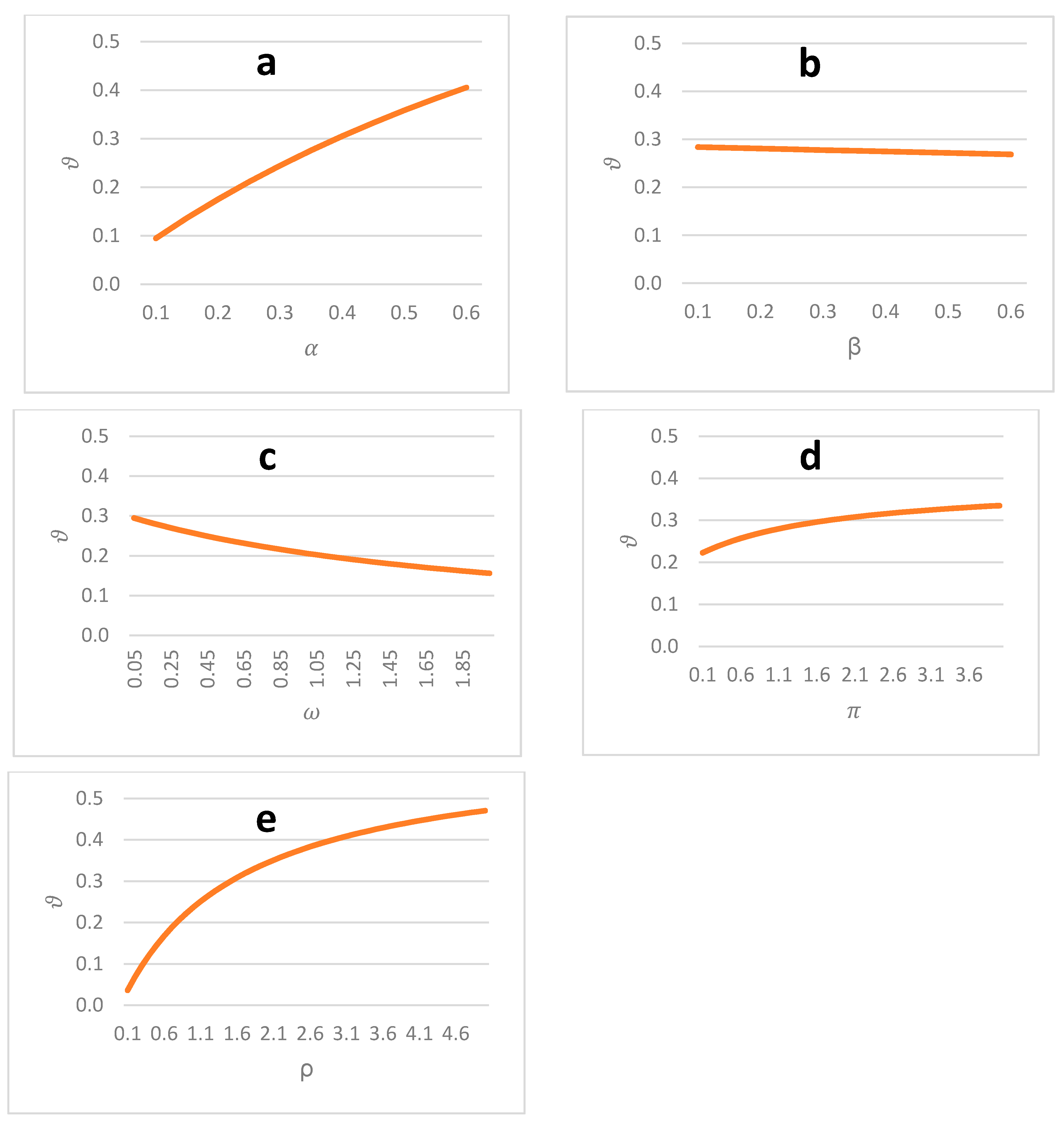
Figure 1 shows the co-movement of the ageing elasticity of energy use w.r.t. each of the key parameters shown in Equation (16) by assuming other parameters taking the values from the literature as given in the beginning of this section. The ageing elasticity of energy use () increases with output elasticity w.r.t. labor () according to Figure 1a. In the Cobb–Douglas production function, the output elasticity w.r.t. labor () can also be explained as labor income share in total output. In an ageing society with less labor inputs relative to capital and energy inputs, the value of should not be more than 0.6 in an economy, although it might be higher in a specific sector such as household services. Hence, for a reasonable value of , the value of the ageing elasticity of energy use () ranges from 0.1 to 0.4.
As shown in Figure 1b, the ageing elasticity of energy use () keeps almost constant (around 0.28) when output elasticity w.r.t. capital () increases from 0.1 to 0.6, indicating the output elasticity of capital () is a relatively modest factor determining the ageing impact on energy use.
For reasonable increases in the labor supply elasticity (), the ageing elasticity of energy use () decreases from 0.30 to 0.15 (Figure 1c). The more elastic labor supply w.r.t. wage rate implies that wage rate may dramatically increase with a small reduction in labor supply caused by population ageing. The increase in wage rate together with full employment in our case leads to dramatic increase in production cost, discourage economic activities and associated energy use. Hence, we obtain smaller impact of population ageing on energy use.
In Figure 1d, the ageing elasticity of energy use () does not increase much (from 0.22 to 0.33) although the capital supply elasticity () dramatically increases from 0.1 to 3.7. Together with the small effect of output elasticity w.r.t. capital (), we can conclude that capital market is relatively less important for the issue of ageing impact on energy use.
The ageing elasticity of energy use () increases markedly from 0.04 to 0.35 when the energy supply elasticity () changes from 0.1 to 2.1. Thereafter, the increase of the ageing elasticity of energy use () slows down (Figure 1e). The population ageing leads to reduction in labor supply, which in turn results in higher wage rate and production cost. If energy use is more elastic to its price, then the same increase in production cost can lead to more reduction in energy use, meaning larger ageing elasticity of energy use ().
To sum up, around the values suggested by previous studies we observe that the ageing elasticity of energy use is generally less than 0.5, meaning 1% reduction in labor supply caused by population ageing reduces energy use by less than 0.5%. The ageing elasticity of energy use is more sensitive to labor elasticity of output () and price elasticity of energy supply () than other parameters of elasticities (, , and ). For all the five parameters, the sensitivity becomes smaller when any of them becomes larger. Based on the results shown in Figure 1, we can conclude that the ageing elasticity of energy use is likely less than 0.5.
5. Conclusions
We have developed an analytical general equilibrium model to explore the population ageing impact on energy use and energy-related emissions via the effect on labor supply. Our results show that 1% reduction in labor supply caused by population ageing results in reduction in energy use by less than 1%, likely smaller than 0.5%. Only in the extreme case of fixed energy supply due to, e.g., strict energy and climate policy, can we expect no reduction in energy use. In that case, population ageing alone is likely to increase energy use and energy-related emissions per capita via effect on labor supply.
Our results indicate that population ageing can result in less energy use and related emissions at a lower rate of the ageing in the long term via labor supply. Based on parameter values suggested in the literature, our rough estimate shows that population ageing may lead to reduction in global energy-related emission in the year 2050 alone roughly equivalent to the yearly emissions in Japan in the recent decade. The accumulated reduction in emissions over time can be considerable.
The impact on energy use is more sensitive to labor elasticity of output and price elasticity of energy supply than other parameters including capital elasticity of output and price elasticities of labor and capital supply. In the future, the energy supply may become more inelastic than today due to strict climate policy and increasing extraction cost of fossil fuels. Hence, the ageing impact on energy use may be diminishing over time. However, renewable energy like solar and wind might not face a stricter cost increase.
These results have to be interpreted by caution since the analytical model is highly abstracted from the real world. For example, in the analysis, the labor supply is assumed the only channel for population ageing to affect the economic activities. This may not be realistic as population ageing can affect economic activities through other channels such as consumption pattern, income redistribution, and investment behavior. We also assume only one consumption goods, which implies constant consumption structure for the whole population. When coming to the energy-related emissions, we assume fixed fossil fuel share in total energy use, which is likely to change in the near future, although mainly driven by factors other than population ageing. Implicitly, we also assume the economy always follows an optimal path for any given external settings.
Acknowledgments
We are grateful for constructive comments by two anonymous referees. This study has been funded by the Research Council of Norway (grant 209701 and 244119). Qin Zhu is also grateful for the financial support from the Major Program of the National Natural Science Foundation of China (Grant 71490735) and the Shanghai Pujiang Program (Grant 16PJC019).
Author Contributions
T. Wei implemented the theoretical analysis; Q. Zhu provided demographic analysis; S. Glomsrød proposed to work on the topic; and all authors wrote the article.
Conflicts of Interest
The authors declare no conflict of interest.
Glossary
| Output in the production activities | |
| Labor input/demand in the production activities | |
| Capital input/demand in the production activities | |
| Energy input/demand in the production activities | |
| Production function | |
| First order derivative w.r.t. any of the arguments in the production function | |
| Secondary derivative w.r.t. any pair of the arguments in the production function | |
| Wage rate | |
| Rental price of capital | |
| Energy price | |
| Labor supply | |
| Capital supply | |
| Energy supply | |
| Labor force at an equilibrium | |
| Capital stock at an equilibrium | |
| Energy use at an equilibrium | |
| Shift parameter due to population ageing in the labor supply function | |
| GHG emissions per unit energy use | |
| Derived expression for energy use at an equilibrium | |
| Derived ageing elasticity of energy use (or energy-related emissions) | |
| Technical parameter in the Cobb–Douglas production function | |
| Output elasticity w.r.t. labor | |
| Output elasticity w.r.t. capital | |
| , , and | Shift parameters in the supply functions of labor, capital and energy, respectively |
| , , and | Price elasticities of supply of labor, capital and energy, respectively |
| and | Elasticities of energy use and capital stock w.r.t. labor input, respectively |
Appendix A
By the supply function (Equations (5)–(7)), the reversed supply function can be written as.
which can be substituted into Equations (2)–(4) to obtain
which holds for any equilibrium of the economy. A change in population ageing (τ) may disturb the economy. To identify the disturbance, total differentiation on both sides of Equation (1) and the above three w.r.t. τ, output, demand and supply of factors yields
which can be rewritten as
To simplify the notation, we define the price elasticity of resource supply:
and the elasticities of marginal product of one factor w.r.t. the factor itself or another factor,
Hence,
Noticing the first-order conditions of the production function (Equations (2)–(4)) and the market clearing conditions (Equations (8)–(10)), we have
Based on the three parts of Equation (A8), we can solve out the elasticity of resources w.r.t. the population ageing parameter,
where
By Equation (13), the population ageing effect on energy-related emissions can be expressed by the elasticity,
If the production function of consumption goods is assumed to be a Cobb–Douglas function as shown in Equation (14), we have
The specific functions for resource supplies expressed in Equation (15) imply that
Substitution of these results in Equation (A11) yields Equation (16) in Section 3.
References
- United Nations Population Division (UNPD). World Population Prospects: The 2015 Revision; United Nations Population Division: New York, NY, USA, 2015. [Google Scholar]
- Auerbach, A.J.; Kotlikoff, L.J. Dynamic Fiscal Policy; Cambridge University Press: Cambridge, UK, 1987. [Google Scholar]
- Miles, D. Modelling the impact of demographic change upon the economy. Econ. J. 1999, 109, 1–36. [Google Scholar] [CrossRef]
- Ludwig, A.; Schelkle, T.; Vogel, E. Demographic change, human capital and welfare. Rev. Econ. Dyn. 2012, 15, 94–107. [Google Scholar] [CrossRef]
- Brounen, D.; Kok, N.; Quigley, J.M. Residential energy use and conservation: Economics and demographics. Eur. Econ. Rev. 2012, 56, 931–945. [Google Scholar] [CrossRef]
- Kronenberg, T. The impact of demographic change on energy use and greenhouse gas emissions in Germany. Ecol. Econ. 2009, 68, 2637–2645. [Google Scholar] [CrossRef]
- O’neill, B.C.; Chen, B.S. Demographic determinants of household energy use in the United States. Popul. Dev. Rev. 2002, 28, 53–88. [Google Scholar]
- Dalton, M.; O’Neill, B.; Prskawetz, A.; Jiang, L.; Pitkin, J. Population aging and future carbon emissions in the United States. Energy Econ. 2008, 30, 642–675. [Google Scholar] [CrossRef]
- Garau, G.; Lecca, P.; Mandras, G. The impact of population ageing on energy use: Evidence from Italy. Econ. Model. 2013, 35, 970–980. [Google Scholar] [CrossRef]
- Wei, T. A general equilibrium view of global rebound effects. Energy Econ. 2010, 32, 661–672. [Google Scholar] [CrossRef]
- Cobb, C.W.; Douglas, P.H. A theory of production. Am. Econ. Rev. 1928, 18, 139–165. [Google Scholar]
- Harcourt, G. Some Cambridge Controversies in the Theory of Capital; CUP Archive: Zurich, Switzerland, 1972. [Google Scholar]
- Wei, T.; Liu, Y. Estimation of resource-specific technological change in a production function. In Proceedings of the Canadian Economics Association Conference 2016, Ottawa, ON, Canada, 3–5 June 2016. [Google Scholar]
- Timmer, M.P.; Dietzenbacher, E.; Los, B.; Stehrer, R.; de Vries, G.J. An Illustrated User Guide to the World Input–Output Database: The Case of Global Automotive Production. Rev. Int. Econ. 2015, 23, 575–605. [Google Scholar] [CrossRef]
- McClelland, R.; Mok, S. A Review of Recent Research on Labor Supply Elasticities; Congressional Budget Office: Washington, DC, USA, 2012.
- Bargain, O.; Peichl, A. Steady-State Labor Supply Elasticities: A Survey; ZEW-Centre for European Economic Research Discussion Paper: Mannheim, Germany, 2013. [Google Scholar]
- Goolsbee, A. Investment Tax Incentives, Prices, and the Supply of Capital Goods. Quart. J. Econ. 1998, 121–148. [Google Scholar] [CrossRef]
- Dahl, C.; Duggan, T.E. U.S. energy product supply elasticities: A survey and application to the U.S. oil market. Res. Energy Econ. 1996, 18, 243–263. [Google Scholar] [CrossRef]
- Van Vuuren, D.P.; Edmonds, J.; Kainuma, M.; Riahi, K.; Thomson, A.; Hibbard, K.; Hurtt, G.C.; Kram, T.; Krey, V.; Lamarque, J.-F.; et al. The representative concentration pathways: an overview. Clim. Chang. 2011, 109, 5–31. [Google Scholar] [CrossRef]
- Le Quéré, C.; Moriarty, R.; Andrew, R.M.; Canadell, J.G.; Sitch, S.; Korsbakken, J.I.; Friedlingstein, P.; Peters, G.P.; Andres, R.J.; Boden, T.A.; et al. Global Carbon Budget 2015. Earth Syst. Sci. Data 2015, 7, 349–396. [Google Scholar] [CrossRef] [Green Version]
Figure 1.
The ageing elasticity of energy use (or energy-related emissions), and key elasticities: elasticity of output with respect to labor (a) and capital (b), price elasticity of labor supply (c), capital supply (d), and energy supply (e).
Figure 1.
The ageing elasticity of energy use (or energy-related emissions), and key elasticities: elasticity of output with respect to labor (a) and capital (b), price elasticity of labor supply (c), capital supply (d), and energy supply (e).
© 2017 by the authors. Licensee MDPI, Basel, Switzerland. This article is an open access article distributed under the terms and conditions of the Creative Commons Attribution (CC BY) license (http://creativecommons.org/licenses/by/4.0/).
Share and Cite
MDPI and ACS Style
Wei, T.; Zhu, Q.; Glomsrød, S. A General Equilibrium View of Population Ageing Impact on Energy Use via Labor Supply. Sustainability 2017, 9, 1534. https://doi.org/10.3390/su9091534
AMA Style
Wei T, Zhu Q, Glomsrød S. A General Equilibrium View of Population Ageing Impact on Energy Use via Labor Supply. Sustainability. 2017; 9(9):1534. https://doi.org/10.3390/su9091534
Chicago/Turabian StyleWei, Taoyuan, Qin Zhu, and Solveig Glomsrød. 2017. "A General Equilibrium View of Population Ageing Impact on Energy Use via Labor Supply" Sustainability 9, no. 9: 1534. https://doi.org/10.3390/su9091534
Note that from the first issue of 2016, this journal uses article numbers instead of page numbers. See further details here.