Temperature Estimation for Photovoltaic Array Using an Adaptive Neuro Fuzzy Inference System


1
Facultad de Ingeniería, Universidad Autónoma de Yucatán, Av. Industrias no Contaminantes, Apdo. Postal 150 Mérida, Yucatán, Mexico
2
Posgrado en Energías Renovables, Facultad de Ingeniería, Universidad Autónoma de Yucatán, Av. Industrias no Contaminantes, Apdo. Postal 150 Mérida, Yucatán, Mexico
*
Author to whom correspondence should be addressed.
Sustainability 2017, 9(8), 1399; https://doi.org/10.3390/su9081399
Submission received: 8 July 2017
/
Revised: 30 July 2017
/
Accepted: 4 August 2017
/
Published: 15 August 2017
(This article belongs to the Special Issue Solar Photovoltaic Electricity)
Abstract
:Module temperature is an important parameter of photovoltaic energy systems since their performance is affected by its variation. Several cooling controllers require a precise estimation of module temperature to reduce excessive heating and power losses. In this work, an adaptive neuro fuzzy inference system technique is developed for temperature estimation of photovoltaic systems. For the learning process, experimental measurements comprising six environmental variables (temperature, irradiance, wind velocity, wind direction, relative humidity, and atmospheric pressure) and one operational variable (photovoltaic power output) were used as training parameters. The proposed predictive model comprises a zero-order Sugeno neuro fuzzy system with two generalized bell-shaped membership functions per input and 128 fuzzy rules. The model is validated with experimental information from an instrumented photovoltaic system with a fitness correlation parameter of R = 95%. The obtained results indicate that the proposed methodology provides a reliable tool for estimation of modules temperature based on environmental variables. The developed algorithm can be implemented as part of a cooling control system of photovoltaic modules to reduce the efficiency losses.
Keywords:
solar energy; temperature photovoltaic cell; photovoltaic performance; sensitivity analysis; artificial intelligence modelingPACS:
J01011. Introduction
Solar energy has become one of the most attractive renewable energy sources since it is abundant, environmentally friendly, and safe. These characteristics have led many countries to pay attention on the design policies, strategies, and technology for its use [1,2,3,4]. In this context, photovoltaic (PV) systems are one of the most mature solar technologies, and it is constantly increasing its competitiveness and decreasing its production costs [5]. For these reasons, PV installations have been considered as a promising alternative to meet the growing demand for electrical energy by the industrial and residential sector [5,6].
On PV systems, the energy conversion process is highly dependent on irradiance. However, irradiance in peak hours produces adverse effects increasing PV module temperature and reducing the module’s performance [7]. A high module temperature produces a reduction of PV efficiency due to the consequent low values of open circuit voltage, fill factor, and power output [8].
Several cooling techniques have been implemented to reduce PV module operating temperature and the consequent efficiency losses [1,9,10]. Nevertheless, in most cases, their implementation requires measurement of the PV temperature using sensors that are usually imprecise. Moreover, the measurement system requires maintenance and calibration, and they are sensitive to climate variations. These factors make them unreliable when the measurement systems are used on a long-term basis [11,12]. An alternative to solve this issue is the use of mathematical and computational models to indirectly estimate the system variables.
Several expressions that correlate PV module temperature as a function of diode PV model electronic parameters (resistance, current, voltage, band gap, etc.) [13], material, and system-dependent properties (glazing-cover transmittance, plate absorptance, etc.) [14], can be found in the relevant literature. In practice, it is complicated to know or obtain the majority of these parameters under long periods of operation. Moreover, it is widely documented that external weather parameters such as environmental temperature, wind speed, wind direction, atmospheric pressure, and relative humidity [15,16,17,18], influence the behavior of PV temperature with high complexity. Therefore, the aim of the present work is the development of an adaptive mathematical model of the PV temperature considering the variability and nonlinear behavior of the environmental parameters [19,20].
In recent years, artificial intelligence (AI) methods have proven to be a powerful tool for nonlinear complex engineering applications. The main advantages of these computational tools are their versatility, robustness, fast computing process, and optimization achieved through learning processes [21,22]. AI methods have been successfully applied in many renewable energy problems [23,24,25,26,27,28,29]. In [23] artificial neural networks (ANN) and genetic algorithms (GA) have been used to predict the thermal efficiency of steam generation plants. Yaïci et al. employed ANN and adaptive neuro fuzzy inference system (ANFIS) for modeling the performance of solar thermal systems [24,25]. Wind speed and wind direction have been forecasted using artificial intelligence algorithms as particle swarm optimization (PSO) and GA [26,27]. Bassam et al. [28] used ANN to estimate the static formation temperatures in geothermal wells. Fuzzy logic algorithms have been employed to design strategies for wind farm efficiency estimation [29].
Among AI modeling methods, adaptive neuro fuzzy inference system (ANFIS) is considered one of the most feasible tools to predict energy systems performance [25]. Several studies on PV technology have been developed using ANFIS. Mellit et al. [30] developed an ANFIS model to predict the optimal sizing coefficient of PV systems based only on geographical coordinates. The results obtained were compared and analyzed with artificial neural networks (ANN) proving that ANFIS model presents the most accurate results. Mohanty [31] generated an ANFIS model to predict monthly solar global radiation for PV system sizing using sunshine duration, ambient temperature, humidity, and clearness index as inputs. The model exhibited an absolute percentage error of 0.48, which yielded better results compared to other methods such as ANN and support vector machine (SVM). Mellit and Kalogirou [32] developed ANFIS models for different components of PV systems such as the generator, battery, and regulator. They designed a global model that combined different ANFIS models relative to each component of the PV system. The components of the global model were trained using various input data. The developed model predicts electrical variables of each component in the PV system using measurements of environmental temperature, irradiation, and clearness index. On the other hand, several studies related to PV maximum power point tracking (MPPT) using ANFIS have been reported in the literature [33,34,35]. These techniques improve the operation efficiency of the systems using input variables as short circuit current (Isc), open circuit voltage (Voc), environmental temperature, irradiation, and others.
In the present work, a new model based on ANFIS methodology to estimate the operation temperature of a PV array is proposed. The rest of this paper is organized as follows: the second section describes the environmental variables that influence the temperature of PV modules, the experimental PV array monitoring, and ANFIS theory. The third section develops the methodology employed in the modeling process by ANFIS technique. The fourth section presents the obtained results, and the last section contains the conclusions.
2. Materials and Methods
2.1. PV Module Performance
In PV industry, the performance of PV modules is evaluated by the standard test conditions (STC), the results of which are reported in the manufacturers’ PV module datasheet. In [13] the PV temperature (TPV) is derived from , where Io is the is the reverse saturation current of the diode PV model, Eg is the band gap of silicon, and B is a temperature-independent constant. Notton el at. [36] described a correlation between PV efficiency () and TPV given by a linear relation (), which depends of reference temperature (Tref), temperature coefficient (), radiation coefficient (), and direct irradiance (Gt). Chow et al. [37] establish a model to estimate the PV array power output () as a function of TPV given by where p is a packing factor and is the glazing transmissivity. Nevertheless, in practice, PV module efficiency is dependent on geographical location and its respective climatological conditions [38]. Several studies indicate that in tropical climates the power supplied by the module in the field can be 30% lower than expected [39]. Among environmental variables that affect the performance of PV module are: temperature (Ta), solar radiation (G), wind velocity (Wv), wind direction (Wd), relative humidity (RH), and atmospheric pressure (Pat).
- Effect of environmental temperature. Similar to other semiconductor devices, solar cells are sensitive to temperature. An increase in temperature reduces the band gap of a semiconductor, affecting most of the semiconductor material parameters. The decrease in the band gap of a semiconductor with increasing temperature can be viewed as an energy increase in the material’s electrons. Lower electronic energy is therefore needed to break the bond, yielding lower current values. In the bond model of a semiconductor band gap, reduction in the bond energy also reduces the band gap. Therefore, increasing the temperature reduces the band gap and consequently its performance. It has been proven that the conversion efficiency of PV modules drops progressively as dust is accumulated on its surface in the simultaneous presence of high temperature [15].
- Effect of solar radiation. Solar radiation is under constant changes throughout the day. It varies depending on geographical location, sun angle, cloudiness, month of the year, etc. An increment of solar radiation improves the module power output, but also increases its temperature, reducing the efficiency [40].
- Effect of wind. The wind lowers the module’s temperature, which helps to reduce the cell temperature, which is crucial to maintaining PV conversion efficiency [16].
- Effect of atmospheric pressure. Atmospheric pressure is a combination of air molecules with weight and movement. The change of air pressure causes the change of airflow on the surface of PV modules, which affects heat dissipation and causes module temperature fluctuation [17].
2.2. Experimental System Description
The experimental system consists of a static PV array located at the Engineering Faculty of the Autonomous University of Yucatan, in Merida, Yucatan, Mexico. It comprises a 4 × 4 PV array built with Siemens SR100 PV monocrystalline modules. The PV modules are south oriented with a tilt angle of 21°. Table 1 summarizes the properties of the PV system.
Experimental data sets were collected during three years in 1-min measurements and 30-min averages to obtain representative samples of several weather conditions. All data was stored using a CR1000 datalogger and the software LoggerNet from the American company Campbell Scientific. The data was filtered to include only measurements obtained between 09:00 and 17:00 hours, corresponding to the location’s peak hours of sunshine. The experimental setup and data acquisition process are illustrated in Figure 1.
Variables measured during the experimental operation were selected according to their influence on PV temperature array. To ensure the accuracy of the measurements, the standard deviations (SD) were computed for each 30-min series. Atmospheric variables, such as solar radiation (G, SD = ±10.13 W/m2), temperature (Ta, SD = ±5.1 °C), wind velocity (Wv, SD = ±0.057 m/s), wind direction (Wd, SD = ±21.12°), relative humidity (RH, SD = ±1.73 %), and atmospheric pressure (Pat, SD = ±0.537 hPa), were measured by a weather station located immediately next to the PV installation. Solar radiation was converted to its equivalent plane-of-array (POA) irradiance to represent the interaction with the tilt of the modules [42]. The temperature of PV array (TPV, SD = ±4.3 °C) was recorded as an average measured by infrared temperature sensors placed in contact with the backside center of the modules. On the other hand, the exposition to atmospheric variables causes a permanent degradation of the cells reducing their performance. Therefore, in the present study the use of PV power output (PPV) as an operational variable for cell degradation assessment is proposed. PV voltage (VPV) and PV current (IPV) of the array were measured to estimate PPV, SD = ±0.4821 W. Table 2 contains the characteristics of employed sensors, which have low uncertainty and, therefore, guarantees data reliability.
2.3. Adaptive Neuro-Fuzzy Inference System (ANFIS)
An adaptive neuro-fuzzy inference system (ANFIS) is a computational technique of the AI family, developed by Jang [43]. ANFIS is a multilayer network combination of ANN learning algorithms and a fuzzy inference system (FIS) to map specific input parameters to an output value. It consists of conventional FIS components (rule base, database, and reasoning mechanism). The neural network’s learning capacity is provided to enhance the system knowledge [25,44]. Computations at each stage are performed by a layer of hidden neurons. There are two FIS types employed in ANFIS modeling called Mamdami and Sugeno, with Sugeno being the most used since it is more computationally efficient and works well with optimization and adaptive techniques [19]. The consequent parameters in Sugeno FIS can be a constant coefficient or a linear equation, called zero-order Sugeno and first-order Sugeno, respectively. Figure 2 illustrates a simple two-rule Sugeno ANFIS architecture with two inputs (x and y) and a single output (F), where A1, A2, B1, and B2 are the input membership functions.
The Sugeno ANFIS model uses fuzzy if-then rules. Equations (1) and (2) express the rules used for the architecture of Figure 2:
where si is the zero-order Sugeno consequent parameter, and pi, qi, and ri are the first-order Sugeno consequent parameters. ANFIS model is composed by a five-layer architecture (Figure 2), where all the nodes in the same layer have a similar function [45]. Layer 1 is composed of membership function nodes. This layer converts the crisped input in fuzzy values, providing the inputs to the following layers. The output of this layer is given by:
where µ is the membership function, O1,i is the membership value for the crisp inputs x and y, and the subscripts 1 and i represent the layer number and node number, respectively.
Layer 2 contains the rule nodes. The nodes in this layer calculate the firing strength of a rule as:
In layer 3, each node calculates the ratio of the i-th rule’s firing strength to the sum of all rule firing strength ():
Layer 4 calculates the rule outputs based on the consequent parameters (Equations (1) and (2)) and the output of the previous layer:
Finally, layer 5 computes the overall output adding all the inputs signals to get the output model value:
3. ANFIS PV Module Modeling
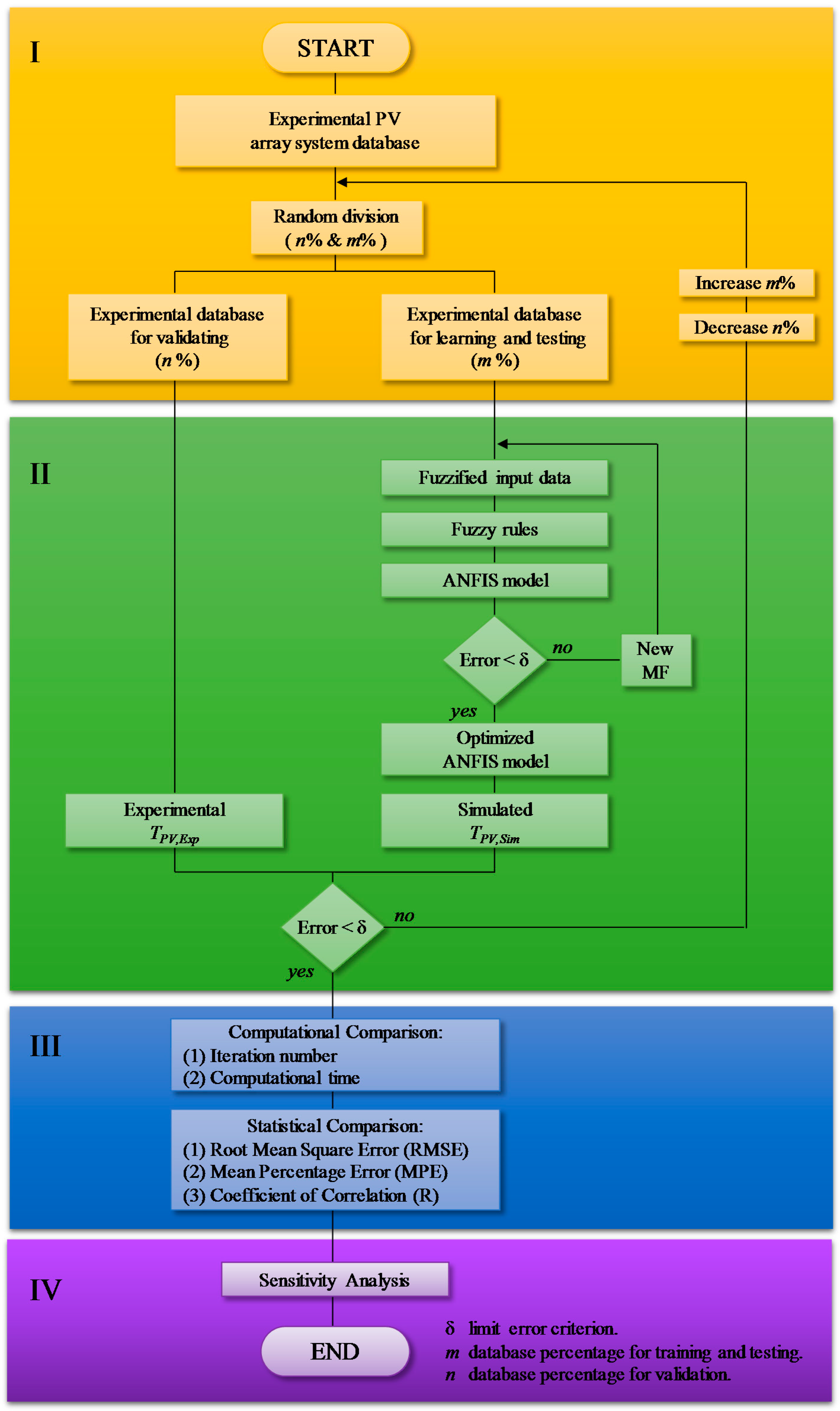
A methodology comprising four steps is employed to estimate the temperature of the PV array considering the influence of atmospheric variables. Figure 3 illustrates a flowchart of the methodology employed.
(I) Database generation using experimental system measurement: The experimental database consists of datasets measured during the experimental system operation described in Section 2. Variables that integrate the database are solar radiation (G, 1367–100 W/m2), temperature (Ta, 39.53–9.56 °C), wind velocity (Wv, 9.80–0.30 m/s), wind direction (Wd, 360–0°), relative humidity (RH, 97–25%), atmospheric pressure (Pat, 103.2–100 Bar), temperature of PV array (TPV, 62.8–9.97 °C), and the PV array output power (PPV, 356–1.5 W). The SD of the variables were included in the database to consider the uncertainty of the measurements. Table 3 enlists the parameters that are part of the database (minimum, nominal and maximum values) and the SD average measurement.
The database was divided randomly into two parts by a systematic sampling to yield an unbiased representation of data set. The first one (m%) was designed for the training process and the second one (n%) was employed for testing and validation. Initial random division starts by assigning half of the database for both processes (m = 50% and n = 50%). To find the better ratio, m% and n% values were increased and decreased, respectively, in steps of 5%. For the current data base, it was found that optimum ratio was presented with m and n values of 85% and 15%, respectively.
(II) Generation of best approximation by ANFIS modeling: An initial ANFIS structure is generated from the seven input variables enlisted in Table 3 to yield the optimum model for temperature prediction of the PV array. The inference system type is defined for the output model behavior, where a zero-order Sugeno model was employed in the modeling process due to the complex nature of PV temperature. Thereby, the evaluation of several combinations of membership functions in the zero-order Sugeno ANFIS structure generated was suggested as a suitable strategy to find the optimum modeling results. On the other hand, the membership function number corresponding to each input variable is chosen heuristically. However, due to the exponential dependency between the total number of rules and the number of input variables membership, the number of functions per input is limited to reduce computational lag.
(III) Computational methodology: To validate the obtained results from ANFIS model, they were compared to the experimental data considering two important aspects: the statistical agreement and the computing performance. Statistical agreement was carried out by a comparison using the three different test parameters illustrated in Table 4, where TPV,Exp is the module temperature, TPV,Sim is the predicted temperature, is the average experimental temperature, is the average simulated temperature, and N indicates the data size. The root mean square error (RMSE) determines the accuracy of the model comparing the deviation of simulated and experimental values. The mean absolute error (MAE) indicates the average quantity of total absolute bias error between estimated and actual values. The coefficient of correlation (R) determines the linear relationship of the predicted data with the measured data [46]. Knowledge of these criteria is relevant to evaluate whether the prediction is sub-estimated or over-estimated with respect to real data.
On the other hand, the computing performance was evaluated considering the optimal epoch and computing time. Optimal epoch is the minimum number of iterations for minimizing the differences between experimental data and the simulated output. Computing time is the one to complete the number of epochs.
(IV) Sensitivity analysis: A sensitivity analysis was performed to determine how the variation of input variables affects the output of ANFIS model. Sensitivity analysis is based on the idea of varying one uncertain parameter to know the response of the model [47]. The analyzed variable is evaluated in the ANFIS model at its maximum and minimum values and maintaining the other input variables in their nominal values. The difference of the output model between the maximum () and minimum () evaluated variable indicates the uncertainly sensitivity range (S):
A larger difference S indicates a larger model sensitivity to the evaluated variable.
4. Results and Discussion
4.1. ANFIS Simulation Results
Training of the ANFIS model is accomplished through a series of epochs performing an optimization process to minimize the differences between experimental data and simulated output. The hybrid learning algorithm (which consists of a combination of the gradient descent method and least squares) was used for the developed model. RMSE results, calculated with experimental data and ANFIS predictions, were used as an optimization criterion for adequacy modeling. Furthermore, ANFIS architecture with two input membership functions was used (generating 128 number of rules) to avoid unnecessary computational load. MATLAB software with its Fuzzy Logic Toolbox [48] was employed to perform the training numerical computations.
Different input membership functions (trimf, trapmf, psigmf, pimf, gaussmf, gauss2mf, and gbellmf) were tested to determine the best ANFIS model. A preliminary training with 550 epochs was carried out to find the number of epochs with the minimum error for each membership function (Figure 4). As it can be appreciated, the best performance is obtained by the bell-shaped membership function (gbellmf).
Table 5 provides the results of computational and statistical criteria for estimation of TPV according to the minimum number of epochs for the membership functions tested. As it can be seen from Table 5, bell-shaped membership function presents the best statistical results (gbellmf, MAE = 0.06729, RMSE = 3.4553, and R = 95.56%), and a low computational time (45.122 s) with the second smallest number of epochs (115).
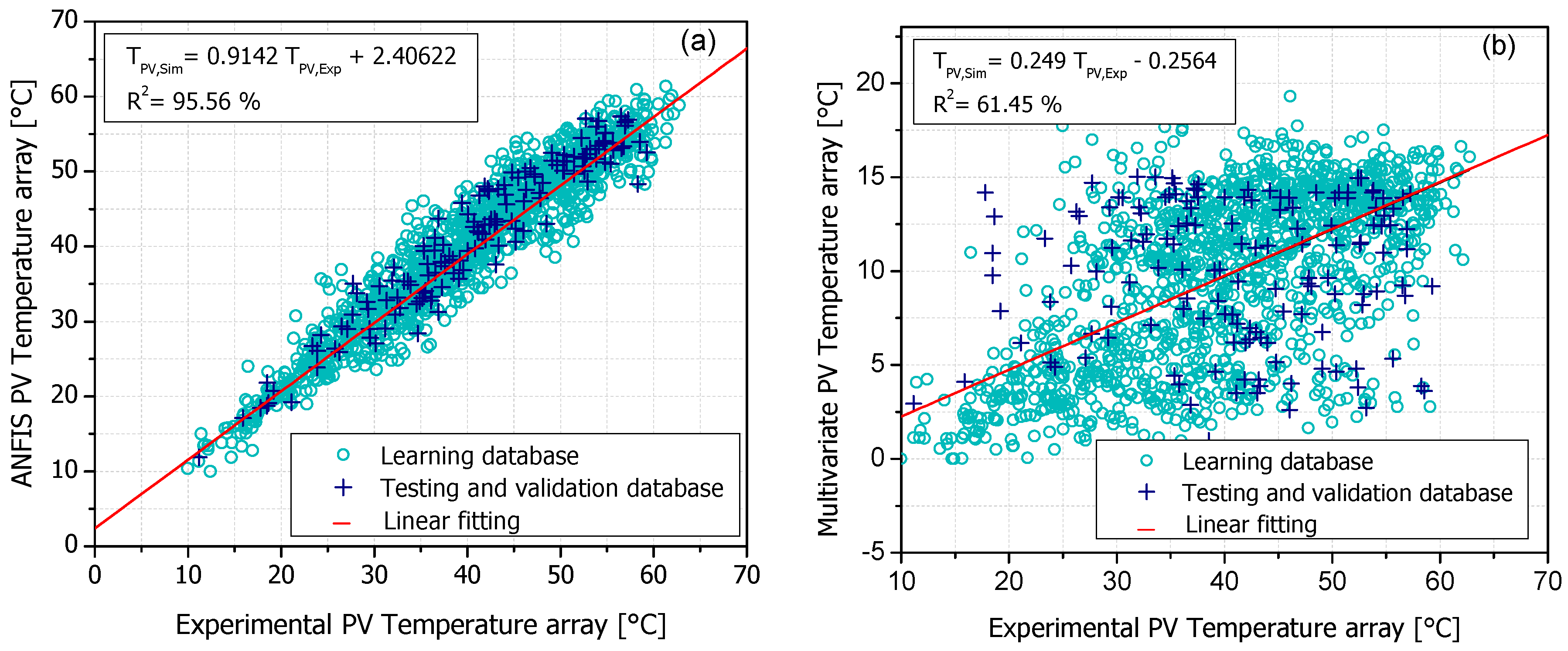
A comparison between ANFIS model and a multivariate regression model was performed to demonstrate the accuracy of the developed model under the same type and number of input variables. Figure 5 illustrates the evaluation of experimental (TPV,Exp) and simulated (TPV,Sim) values for both AI and non-AI modes through a linear regression. The results indicate that the ANFIS model has a significant agreement with the experimental data, obtaining a coefficient R = 0.95563, given by:
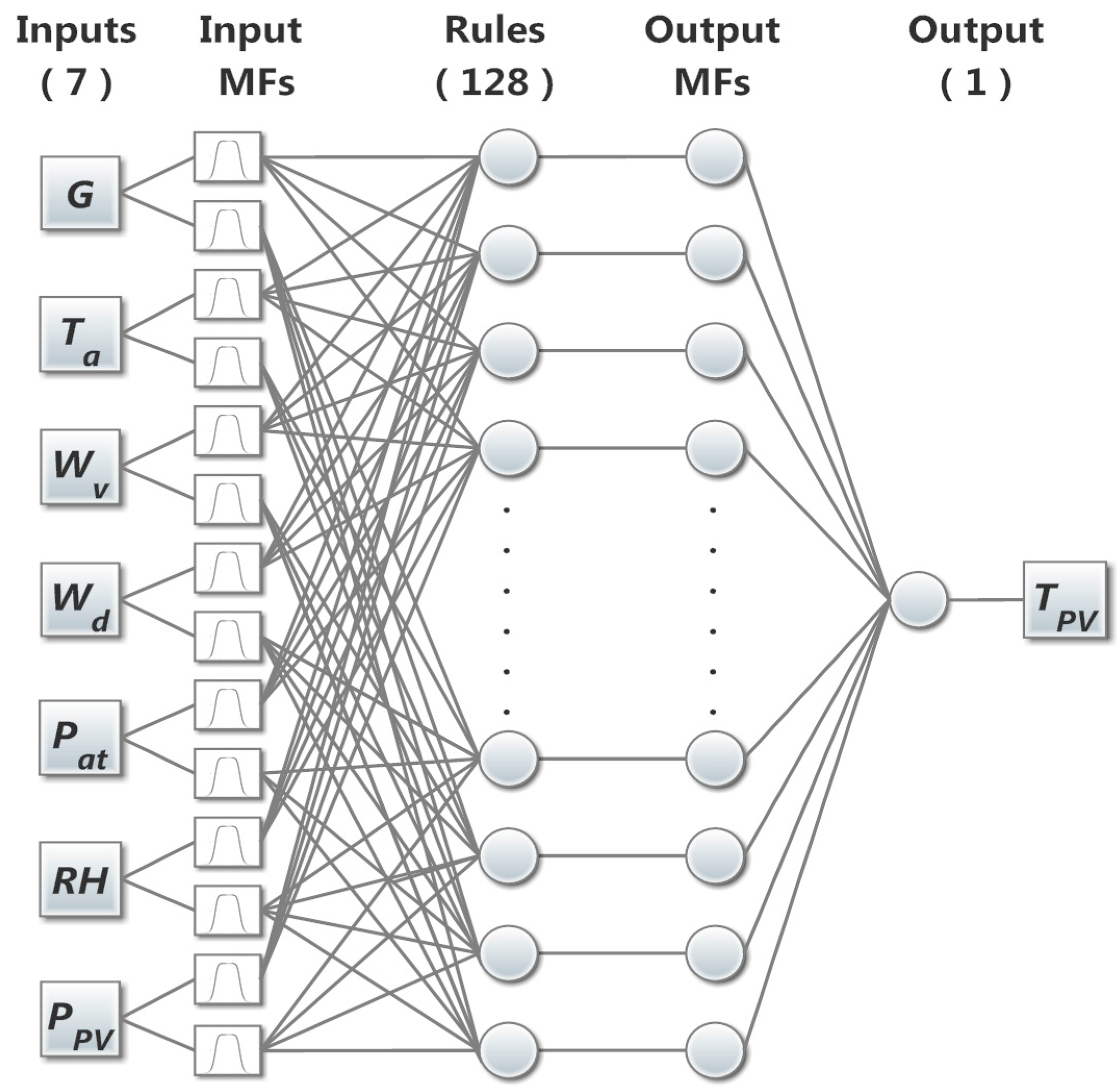
For our implementation, the best zero-order Sugeno ANFIS architecture comprises an input layer with seven nodes, two generalized bell-shaped membership functions per each input node, a rule layer with 128 nodes, an output membership function with 128 constant nodes, and one output corresponding to TPV,Sim (Figure 6).
4.2. Sensitivity Analysis Results
A sensitivity analysis was performed to determine the influence of each input variable to TPV. Moreover, it aims the identification of the positive or negative importance level for the model for each variable. Figure 7 illustrates a tornado chart with the sensitivity analysis results according to the description of Section 3 (IV: Sensitivity analysis). The central value of the graph indicates the TPV at nominal values of input variables (Table 3). On the other hand, the extreme values of Figure 7 represent the TPV variation when evaluating the maximum and minimum values of each input variable. As can be seen, the highest result of the analysis was generated by the environmental temperature, indicating that it is the most influential variable. The second most influential variable according to the sensitivity analysis was the solar radiation, followed by wind velocity, and relative humidity. On the other hand, the wind direction, PV power output, and atmospheric pressure were the variables with less influence.
Even though the wind direction (Wd), PV power output (PPV) and atmospheric pressure (Patm) present a low contribution according to sensitivity analysis, these variables still improve the performance of ANFIS algorithm.
4.3. Evaluation of the ANFIS Model
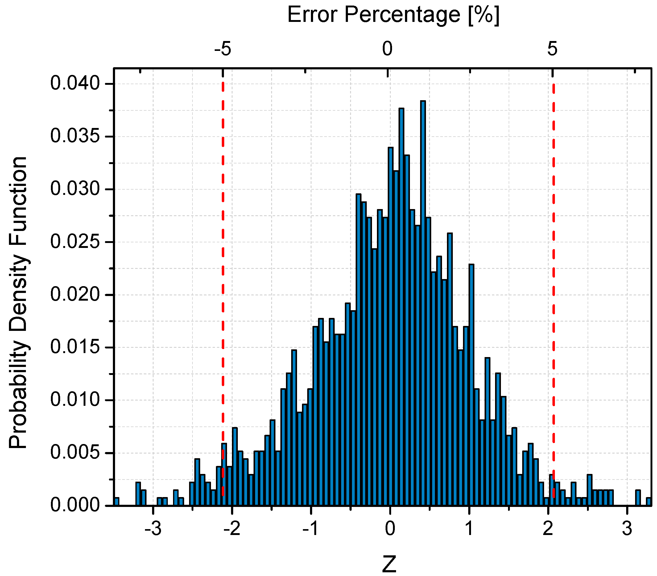
A comparison between experimental and simulated curves of the PV temperature system was performed to validate the developed ANFIS model, employing data not included in the training and testing phases. The comparison criteria employed was the error percentage given by:
The results of the EP evaluation describe an error with a normal distribution behavior, illustrated in the normalized histogram presented in Figure 8. Applying the equation for standard distribution (Z) to histogram results [49] it is possible to establish a correlation between the standard normal distribution and EP. Correlation results indicate that 94% of the EP is in the error percentage range between −5% and 5% (Figure 8), which is an acceptable error for this estimation process according to literature [17,19,42].
The results in Figure 8 indicate that the developed model can estimate the behavior in the temperature of the PV array for different atmospheric conditions. Therefore, the model generates a feasible estimation of the PV array temperature that can be used in monitoring processes and for maximum power control.
Figure 9 illustrates the validation of the ANFIS model for four different cases corresponding to each season of the year. For the validation process, we also included the two most influential variables according to the sensitivity analysis (Ta and G). Case 1, displayed in Figure 9a, describes measurements performed during a clear day with good G levels above 980 W/m2. On the other hand, TPV,Exp curve illustrates high temperature values (above 55 °C between 12:00 and 15:00 hours), which are detrimental to the photovoltaic module performance. These high temperatures are due to the influence of the high levels of G and the Ta that reaches values between 35 °C and 40 °C, being the highest reported in the database. As can be seen in Figure 9a), the estimates of the ANFIS model are able to adapt adequately to the experimental data under clear conditions and gradual changes of Ta.
Case 2 (Figure 9b) considers measurements on a clear day, with a maximum reported radiation rate of 1020 W/m2 between 11:00 and 12:40 hours. However, although solar radiation is higher than in Case 1, Ta has a lower range (20 °C–35 °C), which is due to convective effects of the wind. As illustrated in Figure 9b, TPV,Exp reaches a temperature up to 50 °C between 12:00 and 14:40 hours. These temperatures are lower than those illustrated in Figure 9a, which validate the results of the sensitivity analysis where Ta is more influential on TPV,Exp than G. On the other hand, the estimation of the ANFIS model presents good results to the gradual changes of G and Ta.
Case 3 (Figure 9c) describes a day with high clouds between 12:40 and 14:40 hours. Even though the solar radiation and environmental temperature conditions are not adequate, the TPV,Exp reaches values between 40 °C and 62 °C as a result of latency in temperature increase and influence of other variables described by the sensitivity analysis. As can be observed, the estimation of the model presents errors related to abrupt changes in solar radiation.
Finally, Case 4 (Figure 9d) illustrates the behavior of the PV system temperature for a completely cloudy winter day with radiation (G) lower than 300 W/m2. In the same way, Ta is below 25 °C, which is a favorable condition for the performance of the PV system. It can be observed that at low temperatures (unlike Figure 9b), G has a greater influence on TPV,Exp than Ta. On the other hand, we can see that abrupt fluctuations in solar radiation significantly affect the accuracy of the estimated model generated by ANFIS.
Results in Figure 9 indicate that the developed model is able to estimate the behavior in the temperature of PV array for different atmospheric conditions in a time interval from 09:00 to 17:00 hours. Therefore, the model generates good estimation of the PV modules temperature. The model can be used in the monitoring process and for its implementation in cooling systems to obtain the maximum performance of PV systems.
5. Conclusions
This paper proposed a method to estimate the operation temperature of a photovoltaic array in a specific place considering its power output and atmospheric values. An estimation model for the temperature of a photovoltaic array employing an adaptive neuro fuzzy inference system (ANFIS) was developed. The generated ANFIS model included seven input parameters: solar radiation, environmental temperature, wind velocity, wind direction, relative humidity, atmospheric pressure, and photovoltaic output power. The model was trained with three year experimental database and validated using data not included in the training and testing phase, obtaining a correlation coefficient of 95%. Validation results indicate that the ANFIS model generates good temperature estimations for the photovoltaic array at different atmospheric and operational conditions. Additionally, sensitivity analysis results determine that environmental temperature, solar radiation, wind velocity, and relative humidity are the parameters with the strongest influence on the temperature of the array according to the model.
The methodology and artificial intelligence technique employed proved to be a suitable tool for the estimation of photovoltaic array temperature. The developed ANFIS model provides an alternative to the estimation of photovoltaic temperature based on information generated by meteorological stations. Its use in large-scale photovoltaic installations can generate temperature estimation in a large number of modules, contributing to the reduction of operation, installation and instrumentation costs. In addition, the results of this work contribute to the development of algorithms that improve the photovoltaic systems performance. The implementation of this method in intelligent sensors for photovoltaic cooling systems can be also enhanced. Finally, the results open the door to future works aimed at the study of nonlinear behaviors presented individually in the modules to making reliable estimations that consider adverse situations.
Acknowledgments
The authors thank support of CONACYT on project CONACYT-SENER 254667. The second author thanks CONACYT for the scholarship support.
Author Contributions
All authors contributed equally in the design and performance of the experiments, the analysis of the data and the writing and revision of the manuscript.
Conflicts of Interest
The authors declare no conflict of interest.
References
- Calise, F.; Figaj, R.D.; Vanoli, L. Experimental and Numerical Analyses of a Flat Plate Photovoltaic/Thermal Solar Collector. Energies 2017, 10, 491. [Google Scholar] [CrossRef]
- Tzuc, O.M.; Bassam, A.; Flota-Bañuelos, M.; Ordoñez, E.E.; Ricalde-Cab, L.; Quijano, R.; Vega Pasos, A.E. Thermal Efficiency Prediction of a Solar Low Enthalpy Steam Generating Plant Employing Artificial Neural Networks. In Intelligent Computing Systems; Springer International: Mérida, Yucatán, Mexico, 2016; Volume 4113, pp. 61–73. [Google Scholar]
- Song, A.; Lu, L.; Liu, Z.; Wong, M.S. A Study of Incentive Policies for Building-Integrated Photovoltaic Technology in Hong Kong. Sustainability 2016, 8, 769. [Google Scholar] [CrossRef]
- Cucchiella, F.; Adamo, I.D.; Gastaldi, M. Economic Analysis of a Photovoltaic System: A Resource for Residential Households. Energies 2017, 10, 814. [Google Scholar] [CrossRef]
- Seyboth, K.; Sverrisson, F.; Appavou, F.; Brown, A.; Epp, B.; Leidreiter, A.; Lins, C.; Musolino, E.; Murdock, H.E.; Petrichenko, K.; et al. Renewables 2016 Global Status Report; REN21: Paris, France, 2016. [Google Scholar]
- Kim, S.; Yoon, S.; Choi, W.; Choi, K. Application of Floating Photovoltaic Energy Generation Systems in South Korea. Sustainability 2016, 8, 1333. [Google Scholar] [CrossRef]
- Ceylan, I.; Erkaymaz, O.; Gedik, E.; Gurel, A.E. The prediction of photovoltaic module temperature with artificial neural networks. Case Stud. Therm. Eng. 2014, 3, 11–20. [Google Scholar] [CrossRef]
- Vera, J.T.; Laukkanen, T.; Sirén, K. Multi-objective optimization of hybrid photovoltaic-thermal collectors integrated in a DHW heating system. Energy Build. 2014, 74, 78–90. [Google Scholar] [CrossRef]
- Bahaidarah, H.M.S.; Baloch, A.A.B.; Gandhidasan, P. Uniform cooling of photovoltaic panels: A review. Renew. Sustain. Energy Rev. 2016, 57, 1520–1544. [Google Scholar] [CrossRef]
- Zhang, L.; Chen, Z. Design and Research of the Movable Hybrid Photovoltaic-Thermal (PVT) System. Energies 2017, 10, 507. [Google Scholar] [CrossRef]
- King, D.L.; Kratochvil, J.A.; Boyson, W.E. Temperature coefficients for PV modules and arrays: Measurement/nmethods, difficulties, and results. In Proceedings of the Conference Record of the Twenty Sixth IEEE Photovoltaic Specialists Conference, Anaheim, CA, USA, 29 September–3 October 1997; pp. 1183–1186. [Google Scholar]
- Jordehi, A.R. Parameter estimation of solar photovoltaic (PV) cells: A review. Renew. Sustain. Energy Rev. 2016, 61, 354–371. [Google Scholar] [CrossRef]
- Yordanov, G.H.; Midtgård, O.M.; Saetre, T.O. Series resistance determination and further characterization of c-Si PV modules. Renew. Energy 2012, 46, 72–80. [Google Scholar] [CrossRef]
- Skoplaki, E.; Palyvos, J.A. On the temperature dependence of photovoltaic module electrical performance: A review of efficiency/power correlations. Sol. Energy 2009, 83, 614–624. [Google Scholar] [CrossRef]
- Quaschning, V. Understanding Renewable Energy Systems; Earthscan: London, UK, 2005; Volume 67. [Google Scholar]
- Abiola-Ogedengbe, A.; Hangan, H.; Siddiqui, K. Experimental investigation of wind effects on a standalone photovoltaic (PV) module. Renew. Energy 2015, 78, 657–665. [Google Scholar] [CrossRef]
- Cheng, X.; Chen, F.; Yu, B.; Zhang, X. The method for photovoltaic module temperature ultra-short-term forecasting based on RBF neural network. In Proceedings of the 2016 China International Conference on Electricity Distribution (CICED), Xi’an, China, 10–13 August 2016; pp. 1–5. [Google Scholar]
- Mekhilef, S.; Saidur, R.; Kamalisarvestani, M. Effect of dust, humidity and air velocity on efficiency of photovoltaic cells. Renew. Sustain. Energy Rev. 2012, 16, 2920–2925. [Google Scholar] [CrossRef]
- Dzib, J.T.; Alejos Moo, E.J.; Bassam, A.; Flota-Bañuelos, M.; Escalante Soberanis, M.A.; Ricalde, L.J.; López-Sánchez, M.J. Photovoltaic Module Temperature Estimation: A Comparison Between Artificial Neural Networks and Adaptive Neuro Fuzzy Inference Systems Models. In Intelligent Computing Systems; Springer: Cham, Switzerland, 2016; Volume 597, pp. 46–60. [Google Scholar]
- Schwingshackl, C.; Petitta, M.; Wagner, J.E.; Belluardo, G.; Moser, D.; Castelli, M.; Zebisch, M.; Tetzlaff, A. Wind effect on PV module temperature: Analysis of different techniques for an accurate estimation. Energy Procedia 2013, 40, 77–86. [Google Scholar] [CrossRef]
- Raza, M.Q.; Khosravi, A. A review on artificial intelligence based load demand forecasting techniques for smart grid and buildings. Renew. Sustain. Energy Rev. 2015, 50, 1352–1372. [Google Scholar] [CrossRef]
- Mellit, A.; Benghanem, M.; Kalogirou, S.A. Modeling and simulation of a stand-alone photovoltaic system using an adaptive artificial neural network: Proposition for a new sizing procedure. Renew. Energy 2007, 32, 285–313. [Google Scholar] [CrossRef]
- May Tzuc, O.; Bassam, A.; Escalante Soberanis, M.A.; Venegas-Reyes, E.; Jaramillo, O.A.; Ricalde, L.J.; Ordoñez, E.E.; El Hamzaoui, Y. Modeling and optimization of a solar parabolic trough concentrator system using inverse artificial neural network. J. Renew. Sustain. Energy 2017, 9, 13701. [Google Scholar] [CrossRef]
- Yaïci, W.; Entchev, E. Performance prediction of a solar thermal energy system using artificial neural networks. Appl. Therm. Eng. 2014, 73, 1348–1359. [Google Scholar] [CrossRef]
- Yaïci, W.; Entchev, E. Adaptive Neuro-Fuzzy Inference System modelling for performance prediction of solar thermal energy system. Renew. Energy 2016, 86, 302–315. [Google Scholar] [CrossRef]
- Gao, Y.; Qu, C.; Zhang, K. A Hybrid Method Based on Singular Spectrum Analysis, Firefly Algorithm, and BP Neural Network for Short-Term Wind Speed Forecasting. Energies 2016, 9, 757. [Google Scholar] [CrossRef]
- Zhang, F.; Dong, Y.; Zhang, K. A Novel Combined Model Based on an Artificial Intelligence Algorithm—A Case Study on Wind Speed Forecasting in Penglai, China. Sustainability 2016, 8, 555. [Google Scholar] [CrossRef]
- Bassam, A.; Santoyo, E.; Andaverde, J.; Hernández, J.A.; Espinoza-Ojeda, O.M. Estimation of static formation temperatures in geothermal wells by using an artificial neural network approach. Comput. Geosci. 2010, 36, 1191–1199. [Google Scholar] [CrossRef]
- Petković, D.; Pavlović, N.T.; Ćojbašić, Ž. Wind farm efficiency by adaptive neuro-fuzzy strategy. Int. J. Electr. Power Energy Syst. 2016, 81, 215–221. [Google Scholar] [CrossRef]
- Mellit, A.; Kalogirou, S.A.; Hontoria, L.; Shaari, S. Artificial intelligence techniques for sizing photovoltaic systems: A review. Renew. Sustain. Energy Rev. 2009, 13, 406–419. [Google Scholar] [CrossRef]
- Mohanty, S. ANFIS based Prediction of Monthly Average Global Solar Radiation over Bhubaneswar (State of Odisha). Int. J. Ethics Eng. Manag. Educ. 2014, 1, 2–6. [Google Scholar]
- Mellit, A.; Kalogirou, S.A. ANFIS-based modelling for photovoltaic power supply system: A case study. Renew. Energy 2011, 36, 250–258. [Google Scholar] [CrossRef]
- Aldobhani, A.M.S.; Robert, J. Maximum power point tracking of PV system using ANFIS prediction and fuzzy logic tracking. In Proceedings of the International MultiConference of Engineers and Computer Scientists, Hong Kong, 19–21 March 2008; Vol. II, pp. 19–21. [Google Scholar]
- Vafaei, S.; Gandomkar, M.; Rezvani, A.; Izadbakhsh, M. Enhancement of grid-connected photovoltaic system using ANFIS-GA under different circumstances. Front. Energy 2015, 9, 322–334. [Google Scholar] [CrossRef]
- Kharb, R.K.; Shimi, S.L.; Chatterji, S. Improved Maximum Power Point Tracking for Solar PV Module using ANFIS. Int. J. Curr. Eng. Technol. 2013, 3, 1878–1885. [Google Scholar]
- Notton, G.; Cristofari, C.; Mattei, M.; Poggi, P. Modelling of a double-glass photovoltaic module using finite differences. Appl. Therm. Eng. 2005, 25, 2854–2877. [Google Scholar] [CrossRef]
- Chow, T.T.; He, W.; Ji, J. Hybrid photovoltaic-thermosyphon water heating system for residential application. Sol. Energy 2006, 80, 298–306. [Google Scholar] [CrossRef]
- Micheli, D.; Alessandrini, S.; Radu, R.; Casula, I. Analysis of the outdoor performance and efficiency of two grid connected photovoltaic systems in northern Italy. Energy Convers. Manag. 2014, 80, 436–445. [Google Scholar] [CrossRef]
- Humada, A.M.; Hojabri, M.; Hamada, H.M.; Samsuri, F.B.; Ahmed, M.N. Performance evaluation of two PV technologies (c-Si and CIS) for building integrated photovoltaic based on tropical climate condition: A case study in Malaysia. Energy Build. 2016, 119, 233–241. [Google Scholar] [CrossRef]
- Marion, B.; Adelstein, J.; Boyle, K.; Hayden, H.; Hammond, B.; Fletcher, T.; Canada, B.; Narang, D.; Kimber, A.; Mitchell, L.; et al. Performance parameters for grid-connected PV systems. In Proceedings of the 2005 Conference Record of the Thirty-first IEEE Photovoltaic Specialists Conference, Lake Buena Vista, FL, USA, 3–7 January 2005; pp. 1601–1606. [Google Scholar]
- Elminir, H.K.; Benda, V.; Tousek, J. Effects of solar irradiation conditions on the outdoor performance of photovoltaic modules. J. Electr. Eng. 2001, 52, 125–133. [Google Scholar]
- Lim, L.H.I.; Ye, Z.; Yang, D. Non-contact measurement of POA irradiance and cell temperature for PV systems. In Proceedings of the IECON 2015—41st Annual Conference of the IEEE Industrial Electronics Society, Yokohama, Japan, 9–12 November 2015; pp. 386–391. [Google Scholar]
- Jang, J.S.R. ANFIS: Adaptive-Network-Based Fuzzy Inference System. IEEE Trans. Syst. Man Cybern. 1993, 23, 665–685. [Google Scholar] [CrossRef]
- Mohammadi, K.; Shamshirband, S.; Petkovic, D.; Yee, P.L.; Mansor, Z. Using ANFIS for selection of more relevant parameters to predict dew point temperature. Appl. Therm. Eng. 2016, 96, 311–319. [Google Scholar] [CrossRef]
- Abraham, A. Adaptation of fuzzy inference system using neural learning. Fuzzy Syst. Eng. 2005, 83, 53–83. [Google Scholar]
- Mohammadi, K.; Shamshirband, S.; Kamsin, A.; Lai, P.C.; Mansor, Z. Identifying the most signi ficant input parameters for predicting global solar radiation using an ANFIS selection procedure. Renew. Sustain. Energy Rev. 2016, 63, 423–434. [Google Scholar] [CrossRef]
- Loucks, D.P.; van Beek, E.; Stedinger, J.R.; Dijkman, J.P.M.; Villars, M.T. Water Resources Systems Planning and Management and Applications: An Introduction to Methods, Models and Applications; UNESCO: Paris, France, 2005; Volume 51. [Google Scholar]
- Mathworks, C. Fuzzy Logic ToolboxTM User’s Guide R 2014 b; The MathWorks, Inc.: Natick, MA, USA, 2014. [Google Scholar]
- Spiegel, M.; Stephens, L.J. Theory and Problems of Statistics; McGraw Hill: New York, NY, USA, 2009. [Google Scholar]
Figure 1.
Components of the experimental process.
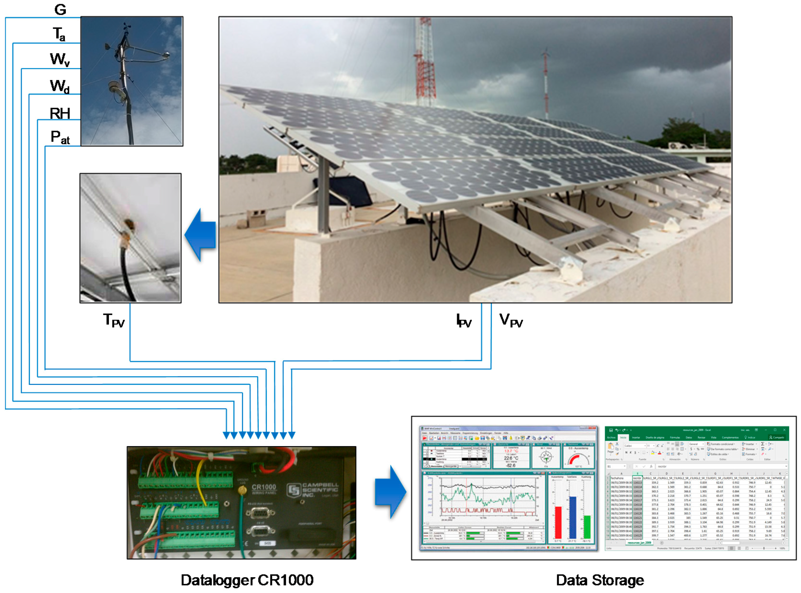
Figure 2.
Simple Sugeno five-layer ANFIS architecture.
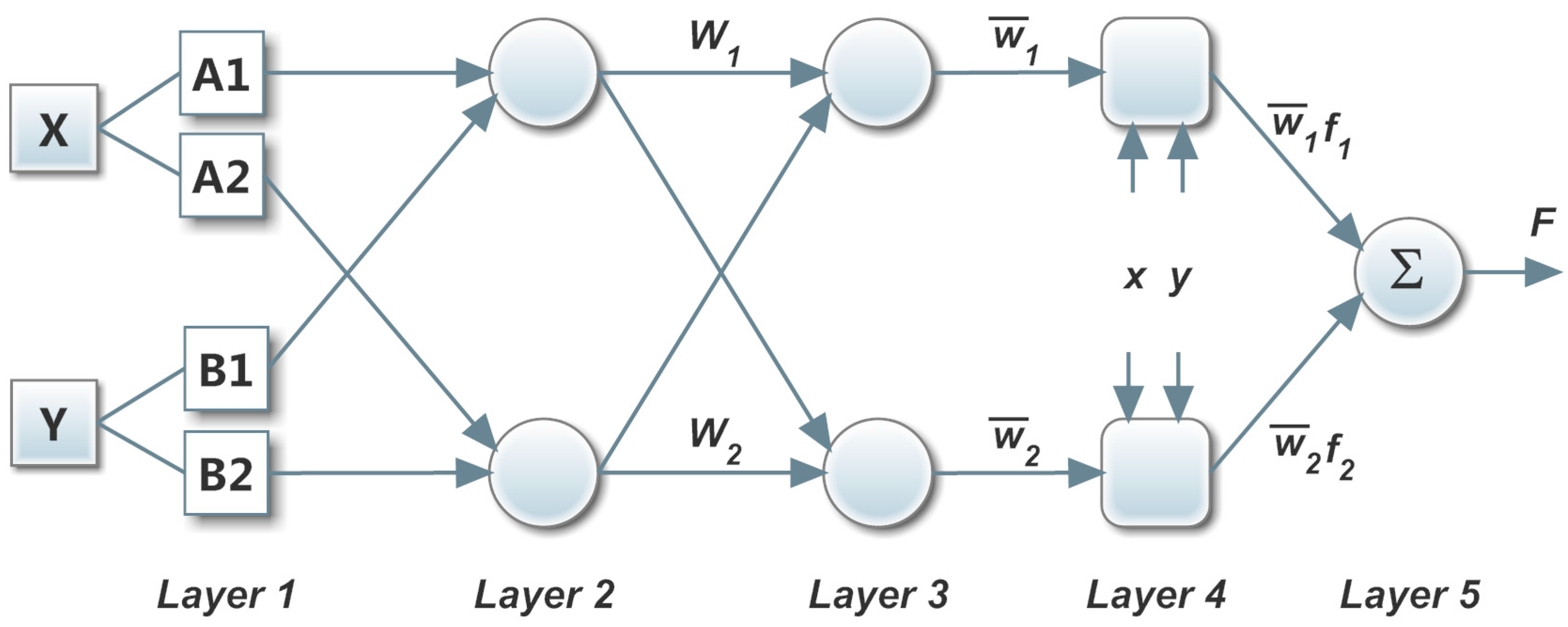
Figure 3.
ANFIS methodology flowchart.

Figure 4.
Evaluation of the seven input membership functions during 550 training epochs.

Figure 5.
Statistical comparison between simulated and experimental PV array temperature. (a) Linear fitting of ANFIS model; and (b) linear fitting of the multivariate regression model.
Figure 5.
Statistical comparison between simulated and experimental PV array temperature. (a) Linear fitting of ANFIS model; and (b) linear fitting of the multivariate regression model.

Figure 6.
ANFIS architecture model for estimation of PV temperature.

Figure 7.
Sensitivity analysis for evaluation of input data importance on the estimation of the PV array temperature using the ANFIS simulation.
Figure 7.
Sensitivity analysis for evaluation of input data importance on the estimation of the PV array temperature using the ANFIS simulation.

Figure 8.
Error percentage normalized distribution probability.

Figure 9.
Comparison of experimental temperature PV array curve and simulated results from the ANFIS model. (a) Model evaluation in a clear day. (b) Model evaluation in the maximum irradiation day reported. (c) Model evaluation in a day with high clouds. (d) Model evaluation in a cloudy winter day.
Figure 9.
Comparison of experimental temperature PV array curve and simulated results from the ANFIS model. (a) Model evaluation in a clear day. (b) Model evaluation in the maximum irradiation day reported. (c) Model evaluation in a day with high clouds. (d) Model evaluation in a cloudy winter day.


Table 1.
Properties of the experimental PV array system.
| Property | Value |
|---|---|
| Latitude (°) | 20°56′ N |
| Longitude (°) | 89°36′ W |
| Tilt angle (°) | 21°00′ |
| Incident area (m2) | 14.16 |
| Nominal output voltage (V) * | 17.7 |
| Nominal output current (A) * | 5.6 |
* According to PV module datasheet.
Table 2.
List of measurement devices.
| Variable | Sensor | Uncertainty |
|---|---|---|
| Solar radiation (G) | Campbell CS300-L Pyrometer | ±5% |
| Environmental temperature (Ta) | Campbell CS215-L | ±4% |
| Wind velocity (Wv) | WINDSONIC4-L | ±2% |
| Wind direction (Wd) | WINDSONIC4-L | ±3% |
| Relative humidity (RH) | Campbell CS215-L | ±4% |
| Atmospheric pressure (Pat) | Campbell CS100 | ±1.0 mb |
| PV voltage (VPV) | TI LM747 | ±5% |
| PV current (IPV) | FW BELL NT-50 | ±0.30% |
| PV temperature module (TPV) | Sensor K-Type | ±0.75% |
Table 3.
Parameters employed for mathematic modeling.
| Parameters | Minimum | Nominal | Maximum | ±SD | Units | |
|---|---|---|---|---|---|---|
| Inputs: | ||||||
| Solar radiation * | (G) | 100 | 987 | 1367 | 10.130 | [W/m2] |
| Temperature | (Ta) | 9.56 | 28.73 | 39.53 | 5.1000 | [°C] |
| Wind velocity | (Wv) | 0.30 | 4.20 | 9.80 | 0.0572 | [m/s] |
| Wind direction | (Wd) | 0 | 133 | 360 | 21.12 | [°] |
| Relative humidity | (RH) | 25 | 57 | 97 | 1.7288 | [%] |
| Atmospheric pressure | (Pat) | 100 | 101.4 | 103.2 | 0.5370 | [hPa] |
| PV output power ** | (PPV) | 17.07 | 326.2 | 356 | 0.4821 | [W] |
| Output: | ||||||
| PV temperature modules | (TPV) | 9.97 | 37.6 | 62.8 | 4.3000 | [°C] |
* Represent the POA irradiation. ** PVP is obtained by the product of VPV and IPV.
Table 4.
Statistical test parameters for ANFIS model evaluation.
| Statistical Criteria | Function |
|---|---|
| Root Mean Square Error | |
| Mean Absolute Error | |
| Coefficient of Correlation |
Table 5.
Results of the ANFIS tested with different membership functions.
| Membership Function | Computational Parameter Criteria | Statistical Analysis | ||||
|---|---|---|---|---|---|---|
| Epochs | Time (s) | (MAE) | (RMSE) | (R) | Best Linear Equation | |
| Trimf | 001 | 0.65000 | 0.07529 | 3.68524 | 0.94293 | Y = 5.99700 + 0.8508X |
| Trapmf | 187 | 93.4484 | 0.07666 | 3.68152 | 0.94314 | Y = 5.99700 + 0.8505X |
| Psigmf | 550 | 386.149 | 0.08790 | 4.26082 | 0.92299 | Y = 5.99717 + 0.8508X |
| Pimf | 550 | 386.950 | 0.07720 | 3.75127 | 0.94080 | Y = 4.56403 + 0.8866X |
| Gaussmf | 437 | 84.2374 | 0.07163 | 3.54318 | 0.94738 | Y = 4.06859 + 0.8996X |
| Gauss2mf | 142 | 69.9605 | 0.07286 | 3.58801 | 0.94425 | Y = 4.12820 + 0.8795X |
| Gbellmf | 115 | 55.7117 | 0.06729 | 3.45530 | 0.95563 | Y = 2.40622 + 0.9142X |
© 2017 by the authors. Licensee MDPI, Basel, Switzerland. This article is an open access article distributed under the terms and conditions of the Creative Commons Attribution (CC BY) license (http://creativecommons.org/licenses/by/4.0/).
Share and Cite
MDPI and ACS Style
Bassam, A.; May Tzuc, O.; Escalante Soberanis, M.; Ricalde, L.J.; Cruz, B. Temperature Estimation for Photovoltaic Array Using an Adaptive Neuro Fuzzy Inference System. Sustainability 2017, 9, 1399. https://doi.org/10.3390/su9081399
AMA Style
Bassam A, May Tzuc O, Escalante Soberanis M, Ricalde LJ, Cruz B. Temperature Estimation for Photovoltaic Array Using an Adaptive Neuro Fuzzy Inference System. Sustainability. 2017; 9(8):1399. https://doi.org/10.3390/su9081399
Chicago/Turabian StyleBassam, A., O. May Tzuc, M. Escalante Soberanis, L. J. Ricalde, and B. Cruz. 2017. "Temperature Estimation for Photovoltaic Array Using an Adaptive Neuro Fuzzy Inference System" Sustainability 9, no. 8: 1399. https://doi.org/10.3390/su9081399
Note that from the first issue of 2016, this journal uses article numbers instead of page numbers. See further details here.