Article

The Effects of Greenbelt Policies on Land Development: Evidence from the Deregulation of the Greenbelt in the Seoul Metropolitan Area

1
Department of Urban and Regional Planning, College of Civil Engineering and Architecture, Zhejiang University, Hangzhou 310058, China
2
Institute of Land Science and Property Management, School of Public Affairs, Zhejiang University, Hangzhou 310058, China
3
Department of Civil and Environmental Engineering, College of Engineering, Seoul National University, Seoul 08826, Korea
4
Jiangxi Institute of Economic Development, Jiangxi Normal University, Nanchang 330022, China
*
Author to whom correspondence should be addressed.
Sustainability 2017, 9(7), 1259; https://doi.org/10.3390/su9071259
Submission received: 5 June 2017 / Revised: 9 July 2017 / Accepted: 12 July 2017 / Published: 18 July 2017
(This article belongs to the Section Sustainable Urban and Rural Development)

Abstract

:
Greenbelt policies are important urban containment policies. On the one hand, they can effectively control the disorderly growth of a city; on the other hand, they can cause other social problems because of their strict control over land development. This paper uses data from 2000 and 2010 and the difference-in-differences (DID) method to evaluate the effects of greenbelt deregulation policies on urban land development in the Seoul metropolitan area (SMA) through a quasi-natural experiment. The results show that first, the deregulation of the greenbelt has significantly furthered urban land development that was not caused by economic development or other factors. Second, the greenbelt deregulation had no significant effects on urban land development in the city centers, but has furthered urban land development near the boundary of Seoul City and greenbelt boundaries. Third, in terms of the effects on land development, the greenbelt deregulation has resulted in regional heterogeneity. Specifically, the greenbelt deregulation has had a significant impact on the urban land development in the southern section of the Han River, whereas the effects of the greenbelt deregulation in the northern area of the Han River are not as obvious.

1. Introduction

With the swift progression of urbanization and the rapid expansion of urban populations, insufficient urban space that is necessary for development has resulted in disorderly city growth, which has led to issues such as traffic congestion, less arable land and less green land [1,2,3,4,5,6,7,8]. Thus, strategies for effectively limiting disorderly urban growth have become a global issue.
Urban containment policies are basic tools of urban space growth management that are widely used to control urban sprawl, to protect open spaces and to shape the growth patterns of urban spaces. There are three main instruments of urban containment policy, namely, greenbelt, urban growth boundary (UGB) and urban service boundaries (USBs) [9,10,11,12]. A greenbelt refers to a physical area of open space, e.g., farmland, forest or other green space, that surrounds a city or metropolitan area, and it is intended to be a permanent barrier to urban expansion. In contrast to greenbelt, a UGB is not a physical space, but a dividing line drawn around an urban area to separate it from surrounding rural areas. USBs delineate the area beyond which certain urban services, such as sewer and water, will not be provided. All three aim to limit future urban growth inside a certain boundary, but the degree of restrictions on urban development declines gradually, and flexibility and complexity of implementation are incremental.
A greenbelt is an ecological urban growth management tool that is different from the UGB and USB. There are usually different kinds of animals and plants in the greenbelt that can improve the atmospheric environment, effectively reduce urban traffic noise, provide habitat of a wild animal protection area, increase bio-diversity, and so on [13,14,15,16]. Meanwhile, the sustainability of urban environments is of increasing concern [17]. It is a necessary condition for the existence of other forms of sustainability [18]. However, past and current urban practices overlook the environmental needs of the community, which violates the global trend to promote sustainable development in the urban areas [19]. Thus, a greenbelt will be also an effective tool for promoting urban environmental sustainability.
It is common to use surrounding greenbelts or embedded “green wedges” to limit the expansion of large cities during development. In the late 1930s, London [20] was the first city in the world to implement a greenbelt policy, followed by Moscow [21], Barcelona, Berlin, Vienna, and Budapest in Europe [22]; Boulder, Ottawa and Toronto in North America [22]; and Seoul, Bangkok, Hong Kong and other cities in Asia.
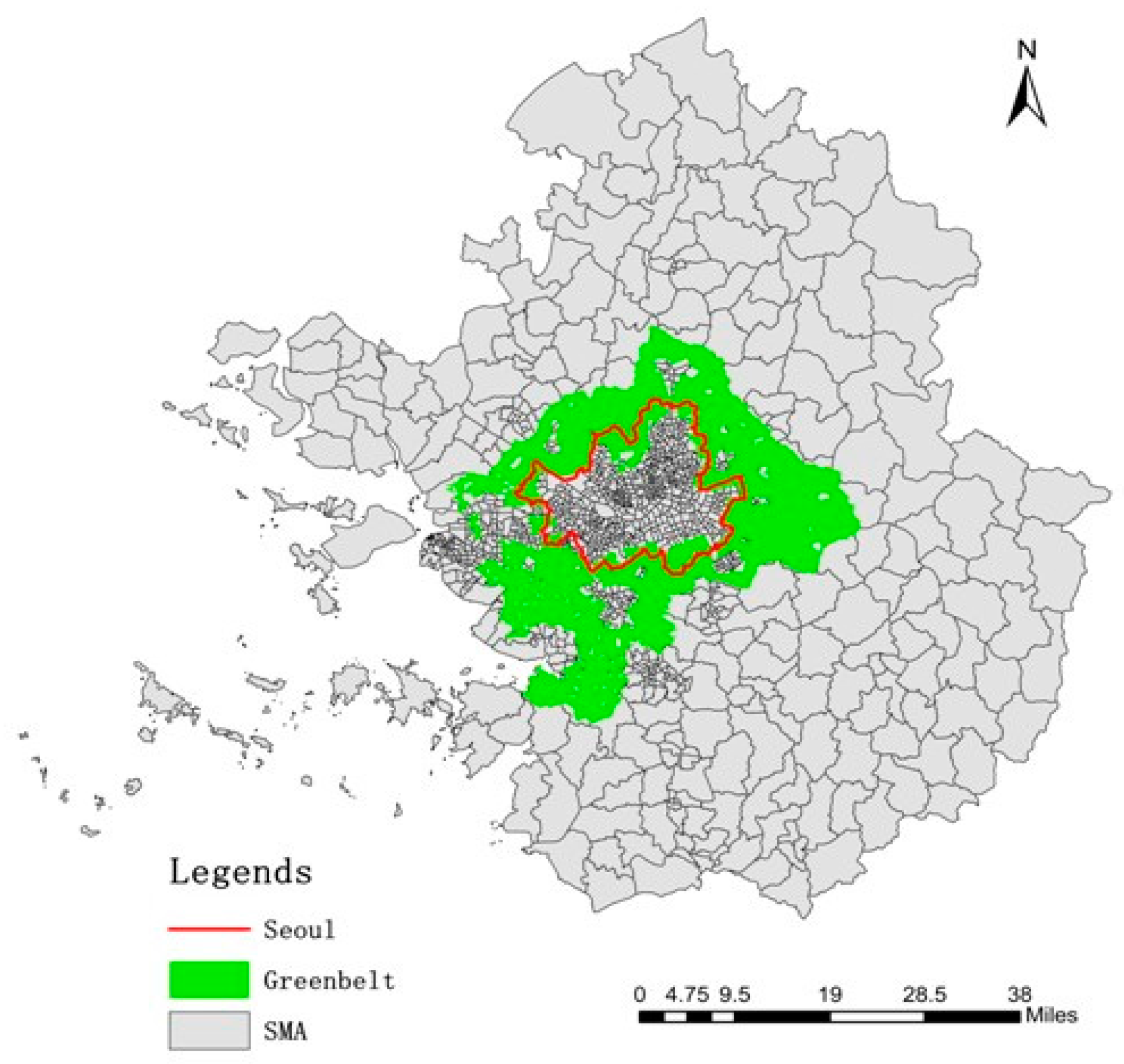
Of the cities that have applied greenbelt policies, the Seoul metropolitan area (SMA) includes the world’s second largest greenbelt, which is also under the most stringent control. Greenbelt policy in South Korea was first known as the concept of “Restricted Development Zones” (RDZs), which was introduced by the Korean military government in the City Planning Law of 1971 and was shaped by the 1972–1981 National Comprehensive Physical Plan of 1973. Greenbelts were built in Seoul and 13 other cities from 1971 to 1987 [23]. Seoul’s greenbelt was patterned after the greenbelt in London, with adjustments according to South Korea’s unique characteristics [24]. The Korean government strictly prohibits any development activities within the greenbelt, and any actions by individuals and enterprises that are contrary to the regulations are severely punished by the government. Because the greenbelt policy was also strictly enforced during the military government era following Park Chung-hee’s term, the greenbelt’s boundaries hardly changed from the 1970s (the setting period) to the 1990s (the democratization period), and activities within it were strictly controlled. The greenbelt’s boundaries were established on the basis of political decision-making rather than on investigation and scientific analysis [25], and various urban problems have emerged to the extent that deregulation pressures have arisen three decades from its initial implementation. In April 1998, the Committee for Green Belt System Improvement, which consisted of 3 greenbelt residents, 1 environmental group representative, 12 scholars, 3 government officials and 3 journalists, was established. In the following 6 months, they developed the trial of improvement plan through investigation, public opinion survey, expert consultation and on-the-spot investigation of greenbelts in the United Kingdom. In June 1999, the final version of the improvement plan was established. Based on the improvement plan, the government analyzed the urban growth patterns, population growth rate and links between the greenbelt and city of the 14 areas (7 big cities and 7 small and medium-sized cities) that implemented greenbelt policies. These cities were divided into two categories: total removal and partial adjustment. With the acceleration of urbanization and the deepening of the suburban housing crisis, in September 2001, the Korean government further confirmed the release of greenbelt areas in seven big cities with high development pressure, and some of these areas were released for development.
In total, 1491 km2 of the whole nation’s greenbelt land (27.68%) and 134 km2 of the SMA’s greenbelt land (8.6%) were released due to the implementation of deregulation from 2000 to 2010. The total released greenbelt area in the SMA covers approximately 134 km2, which accounts for 8.6% of the SMA’s greenbelt. Because half of the country’s population is located in the SMA and the SMA’s greenbelt is representative of greenbelts in Korea, 134 km2 of released greenbelt is rather meaningful, given that the SMA is subject to the heaviest restrictions in terms of military operations, the environment, and growth [26].
Because greenbelt policies in the SMA were formulated early on, studies have made it easy to identify the advantages and disadvantages of such policies. Greenbelt deregulation in the SMA has had a profound impact on the land market, which affects urban land supplies, urban structures and greenbelt accessibility. Consequently, the price of existing land and released greenbelt areas has changed, in addition to resident commuting costs and greenbelt recreation values, which reflect the effects of the greenbelt that restricted land development before and after the application of deregulation.
This paper aims to assess the effect of the deregulation of the greenbelt on land development in the SMA. Firstly, does the deregulation of metropolitan greenbelts increase the probability of urban land development? After the deregulation, was the impact on urban land development in the city centers and land development near the boundary of Seoul and greenbelt boundaries the same? Secondly, is there heterogeneity in the land development probability in different urban areas (the southern part of the Han River and the northern part of the Han River)? To accurately explore the effects of urban containment policies on land development, we used data before the deregulation in 2000 and data after the deregulation in 2010, and adopted a particular approach, the difference-in-differences (DID) method, which treats greenbelt deregulation as a quasi-natural experiment, effectively avoiding the case in the existing research: that greenbelt policy is an exogenous variable.
The rest of the article is organized as follows. First, we review previous research concerning the impact of greenbelt policies on land development in the United States, the United Kingdom and South Korea. Next, we describe the SMA’s greenbelt, detail our research method and set the model. Third, we describe the sources and characteristics of the data. Then, we give the estimation results, make a robust test and discuss these. Finally, we offer concluding remarks.

2. Literature Review

Several scholars have studied the effects of greenbelts on land development. Most of these scholars have concluded that greenbelts have caused an increase in inland prices by strictly restricting land supplies in metropolitan areas. However, specific changes in price vary greatly.
Over the past four decades, American scholars have shown that urban containment policies (such as greenbelt policies) change land and property prices [27,28,29,30,31]. Correll, Lillydahl, and Singell in the United States estimated the value of nearly 3200 feet of land in three greenbelts in Boulder, Colorado. Their results showed a $4.20 decrease in the price of a residential property for every foot that it was away from a greenbelt. The average value of the properties that were adjacent to greenbelts was roughly $54,379, which was higher than the price of areas that were 3200 feet away [32]. Knaap evaluated greenbelt areas in Oregon; Washington; and Caracas, Venezuela, and found that greenbelts have had a significant effect on land values in both counties.
British researchers have shown that, although individuals believe that new housing only accounts for a small portion of the total housing stock, restrictive policies can increase housing prices [33,34,35,36]. Greenbelts have increased housing prices by controlling land supplies, which deeply harms the bottom of the market, as emphasized by the results of Barker’s investigation [37,38]. To some extent, greenbelt policies lead to land price appreciation that benefits landowners and existing landlords, and this increase places more price burdens on renters and buyers [39]. Monk and Whitehead also stated that planning constraints such as greenbelts have reduced the rates of housing construction because of delays in land deregulation and planning approval, and because of increased development costs. As scarcity levels have increased, unit values have appreciated. Individual projects can be subject to damages and can become uneconomical, which reduces housing production. Therefore, restricted planning reduces supplies and drives prices higher [29].
In Korea, an early econometric study by Kim et al. estimated the decrease in housing prices as a result of a relaxation of the greenbelt’s inner edge. They estimated that a 1 km outward movement of the inner edge of the greenbelt, which would add approximately 14% to Seoul’s developable land, would reduce housing prices inbound of Seoul, a subset of the City of Seoul, by 2.7%. This modest decrease in housing prices would be partly due to the relative elasticity of housing demands [40]. Through a simulation, Kim tested the effects of deregulation on housing prices. By releasing approximately 1.2% of Seoul’s greenbelt, Seoul’s supply of residential land could be increased by 1%, assuming that all new land could be used for residential purposes [41]. Choi argued that if greenbelts had been removed in 1987, land prices in greenbelts would have risen by an average of 32.1%, but the price of land outside the greenbelt would have fallen by 7.5%. If the price effects had occurred only within the greenbelt, land prices would have dropped by 19.2%. Son and Kim found that greenbelts, rather than natural restrictions such as mountains, are the main cause of shortages of urban land in Korea. They proposed removing greenbelts to meet the growing demand for urban land and to stabilize land prices in Seoul [42]. Although Bae and Jun did not specifically investigate the land price effects of greenbelts in Seoul, they did indicate that these greenbelts have increased the density of the local population, caused traffic congestion and increased housing prices in the city center [43]. Jeon and Jae Sik, through an analysis of panel data for 2000 to 2010, showed that greenbelt removal has reduced average residential sales prices more in Seoul than in Gyeonggi Province [26]. Hee-Jae Kim and Myung-Jin Jun argued that local greenbelt policies have facilitated urban sprawl by restricting land supplies and by encouraging leapfrog development. Over the past 10 years, greenbelt deregulation has eased housing development pressures in southwestern and northeastern Seoul [44].
The above studies have examined the effects of greenbelt policies on land development, which has great significance. Throughout these studies, researchers have focused on the supply constraining effects of greenbelts by using the hypothesis price model (HPM) and the conditional value evaluation method (CVM) in the early stage as the major empirical methods; the HPM has been used most frequently. However, the HPM method can easily lead to multiple linearity, endogeneity problems and other issues. Land development is caused by a combination of greenbelt policies and other policies. The purposes of greenbelts in each country vary, and problems such as issues of housing affordability and transportation infrastructure accessibility must be considered according to local laws. Thus, the value and the development of land parcels within and outside greenbelt are no longer exogenous factors. Previous studies have disregarded the inner relationships among land development, land prices and land use planning, and laws and regulations. Consequently, few studies have shown whether, through separating the impact of economic development or other factors, land development is influenced by greenbelt policies, let alone the specific effects. In recent studies, the greenbelt effects on land development and housing prices have been analyzed through economic models. These approaches are limited by the simplified nature of the models and by the limits of the analytical methodologies used. Thus, the conclusions of these studies are questionable.

3. Materials and Methods

3.1. Study Site

Seoul is the capital of South Korea and is its national political, economic, cultural and educational center. The total area of South Korea is 605.77 km2; it spans approximately 30.3 km from North to South and approximately 36.78 km from East to West. The urban area is divided into two regions by the Han River: from East to West. In 2013, the population of 25 districts in Seoul reached 10.388 million people, and the population density reached 1.71 million people/km2.
The SMA is one of the world’s super metropolitan areas. The SMA contains Seoul, Gyeonggi-do, Incheon and surrounding areas, and thus covers an area of 11,791 km2. By 2010, Seoul’s metropolitan population reached 24.85 million, which accounted for roughly half of the total population of South Korea. The SMA spans 11,801 km2, and the SMA greenbelt comprises 1424 km2, which accounts for 12.07% of the SMA. The greenbelt area in Seoul covers 153 km2, which is equivalent to 10.75% of the SMA’s greenbelt area. The greenbelt area of Incheon spans approximately 89 km2, which accounts for 6.25% of the SMA’s greenbelt area. The greenbelt area of Gyeonggi Province covers 1182 km2, which accounts for 83% of the SMA’s greenbelt area. By 2010, the SMA population reached 24,857,463, and the population within the greenbelts reached 76,031, which accounted for 0.31% of the SMA’s population (the populations of the greenbelts in Seoul, Incheon, and Gyeonggi-do were 18,039, 2054 and 55,938, respectively). Figure 1 shows greenbelt in SMA.

3.2. Methods

Since the 1980s, economists have developed a particular method that measures policy effects, namely, DID [45]. This method involves a combination of natural science experimentation and statistical science, and regards institutional changes and new policies as “natural experiments”. DID is generally used for public policy evaluations because of its explanatory power and robustness. The DID method needs to satisfy the stochastic hypothesis and the homogeneity hypothesis. To satisfy the stochastic hypothesis, the DID method eliminates the effects of uncontrollable factors by randomization, to control all irrelevant factors that may affect the outcome of the experiment. To satisfy the homogeneity hypothesis, samples in the experimental group and the control group should be one-to-one matched, except for the experimental variables (policy shocks) manipulated by the experimenter, which are different.
Because the greenbelt deregulation in the SMA has reflected processes of quasi-natural experimentation, we used DID to assess the effectiveness of this policy. In theory, greenbelt deregulations should affect greenbelt land development and the development and land use within the entire SMA. Therefore, the land inside the greenbelt could be regarded as the treatment group, while the land outside the greenbelt could be treated as the control group. Technically, the DID method could simultaneously eliminate the differences between the initial values of land parcel development within and outside greenbelts and the impact of time trends on the estimated accuracy levels for each year.

3.3. Model Setting

The DID method involves several steps. First, the treatment group is selected; then, the econometric model is established. This paper considers the land parcels within a greenbelt as the treatment group and treats the areas outside of a greenbelt as the control group. The model settings were as follows:
y i t = α 0 + β 1 g r e e n b e l t i t + β 2 t i m e i t + β 3 d i d i t + γ X i t + e i t
where i and t represent the location and year, respectively, and yit is the dependent variable that represents land development. The changes in land use were used as a proxy variable. According to the principles of land use planning, land uses in the SMA are divided into the eight categories of water, urban land, bare land, wetland, grassland, forest, paddy field and dry land. The changes from water, bare land, wetland, grassland, forest, paddy field, and dry land to urban areas were regarded as forms of land development. The term α0 is a constant. Two dummy variables were established based on a land parcel’s position and the time of the policy implementation; the dummy variable of location is greenbeltit: the land parcels within a greenbelt were defined as 1, and the areas outside a greenbelt were defined as 0. The dummy variable of time is timeit: the periods of time before greenbelt deregulation were defined as 0, and the periods of time after greenbelt deregulation were defined as 1. Different policy effects between the areas within and outside of greenbelt areas were defined as β1, and different policy effects before and after greenbelt deregulation were defined as β2. The interaction between greenbeltit and timeit is didit, which reflects the real policy effects of the greenbelt deregulation on land development, and its coefficient β3 reflects the net effects of greenbelt deregulation on land development. When β3 > 0, the effects of the greenbelt deregulation on land development were positive, and vice versa. The coefficient β3 was significant when the deregulation effects on land development were obvious. Then, the effects of the DID variable on the independent variable could be separated, and we could obtain the concrete policy effects of the greenbelt deregulation. In addition, the vector X is a set of control variables that included elevation, slope, distance to the nearest greenbelt boundary, distance to the nearest city center, distance to the boundary of Seoul City, and distance to the nearest subway, which were confirmed based on the existing research concerning the factors that affect land development [46,47,48,49] (Table 1). Such settings could exclude general factors (e.g., macroeconomic policy, resource endowment, and environmental climate) regarding the effects of land development, and could provide a more accurate assessment of the effects of greenbelt deregulation on land development. The term γ is a vector that contained a set of corresponding parameters, and eit is a random error term.

4. Data Acquisition and Analysis

4.1. Data Acquisition

Use of the DID method has two basic requirements for samples: stochasticity and homogeneity. Thus, we deleted land parcels with abnormal prices that were located in rural areas too far from the greenbelt (outside the outer greenbelt border by 5 km) and in commercial areas (such as the Central Business District and some areas of Gangnam-gu). Then, we selected samples in the remaining land parcels using a simple random sampling method, and determined the sample size using a statistical calculation formula. We obtained 946 land parcels. The greenbelt deregulation was formally applied in 2001; we thus used data from 2000 before the deregulation and from 2010 after the deregulation because samples in the experimental and control groups had to be one-to-one matched. Finally, we obtained 1892 samples from 2000 and 2010.
We studied 1892 samples to explore the effects of the greenbelt deregulation on land development. Table 2 summarizes the data sources of variables. Land parcel data for 2000 and 2010 were drawn from the standard parcels of the Korea Appraisal Board (KAB). In addition, the land use data for 2000 and 2010 were drawn from the Landsat data of the U.S. Geological Survey (USGS). After preprocessing these data, ENVI (The Environment for Visualizing Images) software (Exelis VIS, Tysons Corner, VA, USA) was used to combine the supervised classification and visual interpretation to divide the land uses of the SMA into eight categories. The average elevation data for 2000 and 2010 were drawn from the SRTM (Shuttle Radar Topography Mission), ASTER (Advanced Spaceborne Thermal Emission and Reflection Radiometer) GDEM (Global Digital Elevation Model) digital elevation data of the USGS. The average slope data for 2000 and 2010 were calculated from the digital elevation data. The distances from parcels to the nearest greenbelt boundary, to the boundary of Seoul City, to the nearest city center, and to the nearest subway for 2000 and 2010 were drawn from a digital map that was provided by Seoul National University. We then determined the straight-line distance using ArcGIS software (Esri, Redlands, CA, USA). Data with missing values and errors were removed; after processing the original data, the final available sample included 1878 data points. Moreover, we divided the sample into two parts for the southern section of the Han River and the northern section of the Han River. Accordingly, we obtained 716 samples for the southern section of the Han River and 1162 samples for the northern section of the Han River.

4.2. Descriptive Statistics of the Model Variables

Table 3 summarizes the basic statistics of the variables included in the empirical model. The 1878 samples showed an average elevation of 48.97338 m and a standard deviation (SD) of 0.4 m. The average slope was 6.3°, with a standard deviation of 5.9°. The average distance to the city center was 10,520 m, with a standard deviation of 7542.9 m. The average distance to the boundary of Seoul City was 899.0 m, with a standard deviation of 803.5 m. The average distance to the nearest greenbelt boundary was 1923.4 m, with a standard deviation of 1666.3 m. The average distance to the nearest subway was 2816.2 m, with a standard deviation of 4338.6 m.

5. Results and Discussion

5.1. Model Results

5.1.1. Basic Regression Results and Analysis

We used Stata13 software (StataCorp, College Station, TX, USA) to obtain the following basic analysis results. According to the econometric model, models 1 and 2 of Table 4 estimated the effects of the greenbelt deregulation on land development. In this case, model 1 did not add any control variables and was the most basic DID model. This model only included the constant term (Constant), whether the area was within the greenbelt (Greenbelt), the time before and after greenbelt deregulation (Time) and the average treatment effect (ATE; greenbelt × time). Compared with previous models, model 2 included a set of control variables that related to the economic and social characteristics of urban areas (e.g., the distance to a subway or urban center). The corresponding regression coefficients were described as follows.
(1) Effects of the direction and levels of greenbelt deregulation on land development.
Regarding the coefficient of the ATE in the model, model 1 showed an ATE coefficient of 0.384, which indicated the effects of the greenbelt deregulation on development when no control variable was included in the model. Additionally, this outcome was significant at the 1% level, which showed that greenbelt deregulation accelerated land development and previous greenbelt policies’ control development. The average net growth rate of the development probability for parcels within the greenbelt was 38.4% after the greenbelt deregulation. When the geographic features of a parcel, socio-economic characteristics and other control variables were added to the model, the coefficient of the effects of greenbelt policies on the land development status (ATE) was reduced to 0.329 in model 2, which was still significant at the 1% level. This outcome suggested that inconstant economic and social features and constant geographical features decreased the effects. However, the intensity and direction remained largely stable. Regarding the constant term of the regression models, in model 1, the constant term showed that 76.1% of the land parcels outside the greenbelt had been developed by 2000. The coefficient of initial greenbelt development probability showed that the initial probability of development within the greenbelt was reduced by 48.8%. In model 2, the initial development probability for parcels within the greenbelt was reduced by 33.4%, which was higher than the original probability. The coefficient of time for either model was not significant and was less persuasive (the p-value increased from 0.125 to 0.691). This result indicates that the greenbelt deregulation easily increased the probability of land development, likely because the probability of land development was mainly dependent on the expectations regarding land use change. Normally, greenbelt policies involve strict legal procedures. Compared with local and central government policies and regulations, altering greenbelt policies is significantly more difficult. The changes in greenbelt policies perhaps have a significant impact on an individual’s expectations, which increases the probability of land development.
(2) Effects of the geographical control variables on land development.
The geographical control variables mainly included elevation and slope. In this case, the coefficient of elevation was significant and negative, which indicates that there is a negative relationship between elevation and land development. The land development probability decreased by 0.148% when the elevation increased by 1 m. This relationship had a significant impact on land development in the SMA. An increase in elevation may have increased construction costs. Furthermore, the slope coefficient was very small, while the p-value was 0.620, which suggested that there was no significant correlation between land development and slope. On the one hand, this finding may have been due to fact that the slope of the SMA was gentle. On the other hand, it may have been due to the SMA’s dense population, and individuals may have not minded developing land on a certain slope. Elevation may directly affect the accessibility of traffic facilities and commercial facilities. The higher the elevation, the higher the difficulty of development and the lower the development value. As modern construction technology is highly developed, a slope can be flattened quickly. Thus, the impact of slope on land development was relatively weak. This result was similar to the research of Arthur C. Nelson; in this research, the insignificance of the variable slope may have been explained by the fact that Knox County still had low-slope undeveloped land [49].
(3) Effects of the economic and social control variables on land development.
The distances to the city center had little to do with land development patterns. However, the distance to the boundary of Seoul City was significant at the 1% level, and did not vary with time. In this case, there was a negative relationship between the distance to the boundary of Seoul City and the probability of land development. Land parcels that were closer to the city boundary may have been more likely to become developed. For every 1 km away from the city’s boundaries, the probability of land development decreased by 7.62%. This outcome was inconsistent with our expectations and some previous studies on UGBs. Containment shifts development from exurban and rural areas to suburban and urban areas because of containment boundaries [51,52]. This outcome may have been because UGBs usually surround mono-centric cities, whereas Seoul is a poly-centric city. Mono-centric cities usually occupy the early stages of urban development, and land at the center of these cities is not effectively utilized. Therefore, land development usually occurs at the city center. With city development and the emergence of poly-centric cities, there is often no more space in city centers or the efficiency of land use can no longer improve; thus, land development tends to transmit to the surrounding urban areas. There is also the possibility that the development of urban centers may involve the transformation and demolition of old buildings, making urban centers more expensive to develop than urban boundaries. The distance to the nearest urban subway was negatively correlated with land development in the SMA. In this case, the probability of land development decreased by 1.08% with every kilometer of distance from a subway, although this result was not significant. The effects of the distance to the nearest urban subway on land development varied over time. The coefficient of Dissubway × time was significant at the 10% level. After deregulation, the effects of the distance to the nearest urban subway on land development increased the probability of land development by 1.73%. Model 2 indicated that the effects of the distance to the nearest greenbelt boundary on land development varied over time. The coefficient of Disgb × time was significant at the 5% level. The difference between the periods before and after the greenbelt deregulation was clear. Therefore, land development appeared to be affected by factors that varied over time, although model 1 showed that omitting this variable had no significant effect on the ATE estimation. The coefficient of the distance to the nearest greenbelt boundary was positive, and as the proximity to a greenbelt boundary increased, the probability of land development increased.

5.1.2. Sub-Sample Regression Results and Analysis

The impact of the greenbelt deregulation on land development may have been regionally heterogeneous [26,44]. Therefore, we divided the SMA into two parts, south of the Han River and north of the Han River, and made a comparative study. Table 5 shows that the constant terms for the two sub-regions (north and south of the Han River) were significant at the 1% level. This result suggested that 75.6% of the land parcels outside the greenbelt area in the northern section of the Han River had been developed by 2000, while 41.9% were developed in the southern section of the Han River. The ATE coefficient indicated greenbelt deregulation effect on land development of 0.308 for the northern section of the Han River model, and of −0.483 for the southern section of the Han River model. These results were significant at the 5% level. This outcome suggests that the land development probability in the greenbelt area north of the Han River may increase by 30.8% on average, whereas the land development probability in the greenbelt area south of the Han River may decrease by 48.3% on average. Therefore, the effects of greenbelt deregulation on land development in the northern area of the Han River were more significant than in the southern section of the Han River. The coefficient of the greenbelt in the northern section of the Han River was −0.501, and the coefficient of the greenbelt for the southern section of the Han River was 0.0587; both coefficients were significant. This finding suggests that the initial development probability of the greenbelt in the northern section of the Han River may decrease by 50.1%, and this probability may increase by 5.87% in the southern section of the Han River. The coefficient of time for the northern section of the Han River was not significant, while it was highly significant for the southern section of the Han River. This result indicates that land development in the southern section of the Han River may be heavily affected by the time factor. Under this condition, the parcel development probability of the greenbelt area south of the Han River increased by 76.4% after the greenbelt deregulation.
In Table 6, we added the geographic, economic and social control variables to the model, and discussed the effects of the regional differences that resulted after the greenbelt deregulation on land development in the southern and northern sections of the Han River. The regression coefficient was introduced as follows:
(1) Effects of the direction and levels of greenbelt deregulation on land development.
The constant terms for the southern and northern sections of the Han River were still significant at the 1% level after adding a series of control variables. This result indicated that 80.9% of the land parcels outside the greenbelt in the northern section of the Han River had been developed by 2000, whereas this percentage for the southern section of the Han River only reached 69.2%. These figures were higher than the figures in the basic model described above. The ATE coefficient for the northern section of the Han River was 0.168, and this result was not significant. However, the ATE coefficient for the southern section of the Han River was 0.418, and was significant at the 1% level. Therefore, the greenbelt deregulation seemed to affect the development of the parcels in the greenbelt in the southern section of the Han River. There may have been some political and economic reasons for this phenomenon. Politically, the region north of the Han River is closer to North Korea. For historical reasons, war may occur between South and North Korea in the future. If war were to occur, it would be more difficult to evacuate individuals and materials in this area, and the resulting economic losses would be very high if the government had developed the northern section of the Han River. Thus, the government may be more focused on the development of the southern region. From an economic perspective, this focus is also due to market selection because developers have path dependence for this region and the development potential of the southern section of the Han River is relatively better. In this case, estate developers are more willing to conduct development activities in the southern section of the Han River after the greenbelt deregulation. In 2002, there were 18,793 construction companies in Seoul and 6514 in the northern section of the Han River, while there were 12,279 in the southern section of the Han River. In 2010, the numbers were 19,077, 7100 and 11,977, respectively. In 2002, there were 30,608 real estate and leasing companies in Seoul, 14,121 in the northern section of the Han River and 16,487 in the southern section of the Han River. In 2010, the numbers were 35,100, 15,787 and 19,313 respectively [53,54]. The coefficient of the greenbelt variable was −0.253 (−0.501 before the addition of the control variables) for the northern section of the Han River and −0.366 (0.0587 before the addition of the control variables) for the southern section of the Han River. The effects of deregulation on land development in the greenbelt area south of the Han River changed from positive to negative. This finding showed that, after adding a series of control variables, the initial development probability for the land parcels in the greenbelt areas north of the Han River decreased by 25.3%, and the probability for the southern section of the Han River decreased by 36.6% relative to the land parcels located outside the greenbelt. The coefficient of the Time variable for the northern section of the Han River was not significant, while this coefficient was significant at the 5% level for the southern section of the Han River. This result suggests that land development in the southern section of the Han River may be affected by time. The probability of land parcel development in the southern section of the Han River increased by 16.7% after the greenbelt deregulation.
(2) Effects of the geographical control variables on land development.
The effects of elevation on land development were significantly negative in the two regions. The coefficient of the variable Elevation for the northern section of the Han River was −0.00140, and this coefficient for the southern section of the Han River was−0.00135. Elevation prevents the development and utilization of land. The effects of slope on land development were not significant. The coefficients of the variable Slope for the southern and northern sections of the Han River were small (0.000553 and 0.0000687, respectively), and the p-values (0.878 and 0.981, respectively) were high. Therefore, the slope is unlikely to affect land development in the northern and southern sections of the Han River.
(3) Effects of the economic and social control variables on land development.
The distance to the nearest city center may have a significant impact on the development of land parcels in the southern section of the Han River. In this case, the probability of land development increased by 2.15% with every kilometer of distance from the city center. Following the greenbelt deregulation, this effect was more significant than the effect described above. This probability increased by 2.36% with every kilometer away from the city center. However, the greenbelt deregulation had little effect on land development in the northern section of the Han River. Distance to the boundary of Seoul City had different effects on land development in the two regions. This distance had significant effects on the development of land parcels in the southern section of the Han River. In this region, the probability of land development decreased by 7.75% with every kilometer away from the city boundary, which was slightly higher than the value for the SMA (7.62%). The effects of distance to the nearest greenbelt boundary on land development were significant for both regions, and varied over time. Before the greenbelt deregulation, the probability of land development increased to 10.3% in the northern section of the Han River with every kilometer away from the greenbelt boundary. However, this probability increased to 11.5% in the southern section of the Han River under the same conditions. After the greenbelt deregulation, the probability of land development decreased to 6.74% for the parcels north of the Han River, and to 2.73% for the parcels south of the Han River, with every kilometer away from the greenbelt boundary. In this case, development is more likely to occur near urban and greenbelt boundaries. This result may be due to the presence of an agglomeration economy, and that the land parcels in the central area of the city are highly developed, which decreases the probability of further development. The effects of distance to the nearest urban subway on land development were significant in the southern section of the Han River. The probability of land development decreased by 3.95% with every kilometer from a subway station. However, distance to the nearest urban subway had little impact on land development in the northern section of the Han River. The effects of distance to the nearest urban subway on the land development in the northern and southern sections of the Han River varied overtime. The coefficients of Dissubway × time in the northern and southern sections of the Han River were 0.0800 and 0.0457, respectively, and were both significant at the 1% level. This finding indicated that, after the greenbelt deregulation, the probability of land development increased by 8% in the parcels north of the Han River, and by 4.57% in the parcels south of the Han River.

5.2. Robustness Checks

Whether the improvements in the probability of urban land development were attributable to the greenbelt deregulation or to the expansion of urban areas could be judged from robustness tests. In a study on UGBs in Seattle by Cunningham, a pseudo-UGB was constructed for Seattle’s UGB to test the probability of land development, both within and outside the UGB [55]. This article refers to this practice, and we obtained a new narrow greenbelt by indenting it 500 m from the inner and outer boundaries of the present greenbelt. We used a basic DID model to test our results of the new greenbelt. Table 7 shows the results of robustness checks. Our results indicated that after the greenbelt boundaries were indented by 500 m, the greenbelt deregulation still improved the probability of land development in the greenbelt. In addition, the effects of time on land development became significant, which suggested that the greenbelt deregulation was the real cause of increases in land development probability. This outcome supported the results that are shown above.
Although important discoveries were revealed by these studies, there were also limitations. This study used a new approach to measure the impact of greenbelt policies on land development, and the study was conducted in the context of South Korea. The results may be completely different in other countries that implement greenbelt policies. This may be similar to the evaluation results of the UGB.
There were also some limitations in the methods. First, using the DID method, we could infer whether the change of policy significantly influenced our sample, but we could not judge how the effect intensity changed over time. Second, the conventional DID estimation is only applicable to linear relationships. When there is a non-linear relationship or a non-random selection of the sample, this method is not applicable. In this case, it is more reasonable to choose semiparametric and nonparametric methods to assess the effectiveness of the policy [56]. The traditional DID method requires samples in the experimental and control groups be one-to-one matched, except for the experimental variables (policy shocks) manipulated by the experimenter, which are different. When two groups of samples are not one-to-one matched, a synthetic control method may be better [57].
Given the limits of our data, the research of this paper was not deep enough; we divided Seoul into only the southern and northern part of the Han River. In fact, the impact of the deregulation of the greenbelt may have been different in every district; future research can be carried out regarding this aspect to obtain more meaningful conclusions. In the future, we can also divide land development into different types, such as by dividing the urban area into residential, commercial and industrial areas, to further study the effect of deregulation on land development.

6. Conclusions

Recognizing and understanding the relationships between urban containment policies and urban land development is crucial. This understanding relates to the reasonable design of internal urban structures as well as to the strategic planning of urban management systems. Therefore, the relationships between urban design and urban planning were attractive subjects of study. This paper adopts data from 2000 and 2010, and uses a DID method to evaluate the greenbelt deregulation effects on urban land development in the SMA through a quasi-natural experiment. The results indicate that greenbelt policies in the SMA have had a significant impact on urban land development, and that greenbelt deregulation has no significant effects on urban land development in the central area of the city, but increases the probability of urban land development in the areas that surround the urban administrative and greenbelt boundaries. In this work, we also compare the effects of the greenbelt deregulation on land development in the southern and northern section of the Han River. The greenbelt deregulation has a significant impact on the urban land development in the southern section of the Han River.

Acknowledgments

This research was supported by the International Scholar Exchange Fellowship (ISEF) of Korea Foundation for Advanced Studies, National Natural Science Foundation of China (51278526, 71403248), Zhejiang Province Zhejiang Youth Project (T2-2, 11ZJQN029YB), Department of Science & Technology of Zhejiang Province (2016C35003).

Author Contributions

This research was completed by the authors collaboratively. Haoying Han conceived the study idea. Chen Huang developed the research methodology, analyzed the data, and wrote most of the paper. Kun-Hyuck Ahn and Haoying Han provided data and directed and approved the study. Xianfan Shu, Liyun Lin and Derong Qiu revised the study.

Conflicts of Interest

The authors declare no conflict of interest.

References

  1. Anas, A.; Rhee, H.J. Curbing excess sprawl with congestion tolls and urban boundaries. Reg. Sci. Urban Econ. 2006, 36, 510–541. [Google Scholar] [CrossRef]
  2. Glaeser, E.L.; Kahn, M.E. Sprawl and urban growth. Handb. Reg. Urban Econ. 2004, 4, 2481–2527. [Google Scholar]
  3. Bruegmann, R. Sprawl: A compact history. Mobility 2005, 96, 666–667. [Google Scholar]
  4. Zhou, X.; Wang, Y.C. Spatial-temporal dynamics of urban green space in response to rapid urbanization and greening policies. Landsc. Urban Plan. 2011, 100, 268–277. [Google Scholar] [CrossRef]
  5. Macdonald, K.; Rudel, T.K. Sprawl and forest cover: What is the relationship? Appl. Geogr. 2005, 25, 67–79. [Google Scholar] [CrossRef]
  6. Ewing, R.; Pendall, R.; Chen, D. Measuring sprawl and its impact. Smart Growth Am. 2002, 57, 320–326. [Google Scholar]
  7. Centre, D.G.J.; Agency, E.E. Urban Sprawl in Europe: The Ignored Challenge. Available online: https://doi.org/10.1080/02697451003740312 (accessed on 1 June 2017).
  8. Brueckner, J.K. Urban sprawl: Diagnosis and remedies. Int. Reg. Sci. Rev. 2000, 23, 160–171. [Google Scholar] [CrossRef]
  9. Pendall, R.; Martin, J.; Fulton, W.B. Holding the line: Urban containment in the United States. Brooks Instrum. 2002, 1, 18–24. [Google Scholar]
  10. Bengston, D.; Youn, Y.-C. Urban containment policies and the protection of natural areas: The case of Seoul’s greenbelt. Ecol. Soc. 2006, 11, 3. [Google Scholar] [CrossRef]
  11. Hall, P. The containment of urban England. Geogr. J. 1974, 140, 386–408. [Google Scholar] [CrossRef]
  12. Haoying, H.; Ke, F.; Cifang, W. Urban containment policy: A global experience. J. Zhejiang Univ. Human. Soc. Sci. Ed. 2009, 39, 162–171. (In Chinese) [Google Scholar]
  13. Bosetti, V.; Locatelli, G. A data envelopment analysis approach to the assessment of natural parks’ economic efficiency and sustainability. The case of Italian national parks. Sustain. Dev. 2006, 14, 277–286. [Google Scholar] [CrossRef]
  14. Pathak, V.; Tripathi, B.D.; Mishra, V.K. Evaluation of anticipated performance index of some tree species for green belt development to mitigate traffic generated noise. Urban For. Urban Green. 2011, 10, 61–66. [Google Scholar] [CrossRef]
  15. Sandstrom, U.G.; Angelstam, P.; Mikusinski, G. Ecological diversity of birds in relation to the structure of urban green space. Landsc. Urban Plan. 2006, 77, 39–53. [Google Scholar] [CrossRef]
  16. Shannigarhi, A.S.; Fukushima, T.; Sharma, R.C. Anticipated air pollution tolerance of some plant species considered for green belt development in and around an industrial/urban area in India: An overview. Int. J. Environ. Stud. 2004, 61, 125–137. [Google Scholar] [CrossRef]
  17. Keirstead, J.; Leach, M. Bridging the gaps between theory and practice: A service niche approach to urban sustainability indicators. Sustain. Dev. 2008, 16, 329–340. [Google Scholar] [CrossRef]
  18. Bithas, K.P.; Christofakis, M. Environmentally sustainable cities. Critical review and operational conditions. Sustain. Dev. 2006, 14, 177–189. [Google Scholar] [CrossRef]
  19. Chan, E.H.W.; Lee, G.K.L. Contribution of urban design to economic sustainability of urban renewal projects in Hong Kong. Sustain. Dev. 2008, 16, 353–364. [Google Scholar] [CrossRef]
  20. Munton, R.J.C. London’s Green Belt: Containment in Practice; Routledge: Abingdo, UK, 1983. [Google Scholar]
  21. Boentje, J.P.; Blinnikov, M.S. Post-Soviet forest fragmentation and loss in the green belt around Moscow, Russia (1991–2001): A remote sensing perspective. Landsc. Urban Plan. 2007, 82, 208–221. [Google Scholar] [CrossRef]
  22. Kühn, M. Greenbelt and Green Heart: Separating and integrating landscapes in European city regions. Landsc. Urban Plan. 2003, 64, 19–27. [Google Scholar] [CrossRef]
  23. Bae, C.-H.C. Korea’s greenbelts: Impacts and options for change. Pac. Rim Law Policy Assoc. 1998, 7, 479–502. [Google Scholar]
  24. Bengston, D.N.; Yeo-Chang, Y. Seoul’s Greenbelt: An Experiment in Urban Containment. Available online: https://core.ac.uk/download/pdf/51180716.pdf (accessed on 1 June 2017).
  25. Jun, M.-J.; Bae, C.-H.C. Estimating the commuting costs of Seoul’s greenbelt. Int. Reg. Sci. Rev. 2000, 23, 300–315. [Google Scholar] [CrossRef]
  26. Sik Jae, J. The Effect of Greenbelt Policy Reform on the Seoul Metropolitan Area Housing Market. Available online: http://smartgrowth.umd.edu/assets/documents/acsp/acsp2012paper_jeon.pdf (accessed on 1 June 2016).
  27. Knaap, G.J. The price effects of urban growth boundaries in metropolitan Portland, Oregon. Land Econ. 1985, 61, 26–35. [Google Scholar] [CrossRef]
  28. Nelson, A.C. Using land markets to evaluate urban containment programs. J. Am. Plan. Assoc. 1986, 52, 156–171. [Google Scholar] [CrossRef]
  29. Landis, J.D. Land regulation and the price of new housing lessons from three California cities. J. Am. Plan. Assoc. 1986, 52, 9–21. [Google Scholar] [CrossRef]
  30. Shilling, J.D.; Sirmans, C.F.; Guidry, K.A. The impact of state land-use controls on residential land values. J. Reg. Sci. 1991, 31, 83–92. [Google Scholar] [CrossRef]
  31. Katz, L.; Rosen, K.T. The interjurisdictional effects of growth controls on housing prices. J. Law Econ. 1987, 30, 149–160. [Google Scholar] [CrossRef] [Green Version]
  32. Correll, M.R.; Lillydahl, J.H.; Singell, L.D. The effects of greenbelts on residential property values: Some findings on the political economy of open space. Land Econ. 1978, 54, 207–217. [Google Scholar] [CrossRef]
  33. Evans, A. The determination of the price of land. Urban Stud. 1980, 20, 119–129. [Google Scholar] [CrossRef]
  34. Cheshire, P.; Sheppard, S. British planning policy and access to housing: Some empirical estimates. Urban Stud. 1989, 26, 469–485. [Google Scholar] [CrossRef]
  35. Bramley, G. Land-use planning and the housing market in Britain: The impact on house building and house prices. Environ. Plan. A 1993, 25, 1021–1051. [Google Scholar] [CrossRef]
  36. Monk, S. Evaluating the economic impact of planning controls in the United Kingdom: Some implications for housing. Land Econ. 1999, 75, 74–93. [Google Scholar] [CrossRef]
  37. Adams, D.; Watkins, C. Greenfields, Brownfields and Housing Development; Blackwell: Somerset County, NJ, USA, 2008. [Google Scholar]
  38. Bramley, G.; Bartlett, W.; Lambert, C. Planning, the Market and Private House-Building; UCL: London, UK, 1995. [Google Scholar]
  39. Barker, K. Barker Review of Housing Supply. Available online: http://webarchive.nationalarchives.gov.uk/+/http://www.hm-treasury.gov.uk/barker_review_of_housing_supply_recommendations.htm (accessed on 1 June 2017).
  40. Kim, K.H. An Analysis of Inefficiency of an Urban Housing Market: The Case of Seoul, Korea; Princeton University: Princeton, NJ, USA, 1987. [Google Scholar]
  41. Kim, K.H. Housing prices, affordability, and government policy in Korea. J. Real Estate Financ. Econ. 1993, 6, 55–71. [Google Scholar] [CrossRef]
  42. Son, J.Y.; Kim, K.H. Analysis of urban land shortages: The case of Korean cities. J. Urban Econ. 2005, 43, 362–384. [Google Scholar] [CrossRef]
  43. Bae, C.H.C.; Jun, M.J. Counterfactual planning: What if there had been no greenbelt in Seoul? J. Plan. Educ. Res. 2003, 22, 374–383. [Google Scholar] [CrossRef]
  44. Kim, H.J.; Jun, M.J. Measuring the Effects of the Greenbelt Policy on Urban Residential Development. Available online: http://www.dbpia.co.kr/Journal/ArticleDetail/NODE06614240 (accessed on 1 June 2017).
  45. Abadie, A. Difference-in-Difference Estimators; Palgrave Macmillan: Basingstroke, UK, 2010. [Google Scholar]
  46. Dempsey, J.A.; Plantinga, A.J. How well do urban growth boundaries contain development? Results for Oregon using a difference-in-difference estimator. Reg. Sci. Urban Econ. 2013, 43, 996–1007. [Google Scholar] [CrossRef]
  47. Cho, S.H.; Poudyal, N.; Lambert, D.M. Estimating spatially varying effects of urban growth boundaries on land development and land value. Land Use Policy 2008, 25, 320–329. [Google Scholar] [CrossRef]
  48. Cho, S.H.; Omitaomu, O.A.; Poudyal, N.C.; Eastwood, D.B. The impact of an urban growth boundary on land development in Knox County, Tennessee: A comparison of two-stage probit least squares and multilayer neural network models. J. Agric. Appl. Econ. 2007, 39, 701–717. [Google Scholar] [CrossRef]
  49. Nelson, A.C. An empirical note on how regional urban containment policy influences an interaction between greenbelt and exurban land markets. J. Am. Plan. Assoc. 1988, 54, 178–184. [Google Scholar] [CrossRef]
  50. U.S. Geological Survey. Available online: https://glovis.usgs.gov/ (accessed on 14 July 2017).
  51. Nelson, A.C.; Burby, R.J.; Feser, E.; Dawkins, C.J.; Malizia, E.E.; Quercia, R. Urban containment and central-city revitalization. J. Am. Plan. Assoc. 2004, 70, 411–425. [Google Scholar] [CrossRef]
  52. Cho, S.H.; Chen, Z.; Yen, S.T.; Eastwood, D.B. Estimating effects of an urban growth boundary on land development. J. Agric. Appl. Econ. 2006, 38, 377–391. [Google Scholar] [CrossRef]
  53. Korean Statistical Information Service. Available online: http://kosis.kr/statHtml/statHtml.do?orgId=101&tblId=DT_1KI2002&language=en&conn_path=I3 (accessed on 1 June 2017).
  54. Seoul Metropolitan Government. Available online: http://seoul-e.lhsoft.co.kr/get-to-know-us/statistics-of-seoul/seoul-statistics-by-category/ (accessed on 1 June 2017).
  55. Cunningham, C.R. Growth controls, real options, and land development. Rev. Econ. Stat. 2007, 89, 343–358. [Google Scholar] [CrossRef]
  56. Abadie, A. Semiparametric difference-in-differences estimators. Rev. Econ. Stud. 2005, 72, 1–19. [Google Scholar] [CrossRef]
  57. Abadie, A.; Diamond, A.; Hainmueller, J. Comparative politics and the synthetic control method. Am. J. Political Sci. 2015, 59, 495–510. [Google Scholar] [CrossRef]
Figure 1. SMA greenbelt.
Sustainability 09 01259 g001
Table 1. Definitions of the major variables.
Variable NameVariable SignVariable DefinitionReferences
Dependent Variable
Changesin land useyLand use changes are defined as 1;
no change is defined as 0.
[46,47,48]
Independent Variable
Effects of greenbelt deregulation (core independent variable)didThe real impact of the greenbelt deregulation on land development.[46]
Land parcel position variableGreenbeltThe area withina greenbelt is defined as 1; the area outside a greenbelt is defined as 0.[47,48,49]
Policy implementation time variableTimeThe period before greenbelt deregulation is defined as 0; the period after greenbelt deregulation is defined as 1.[46]
Geographical control variable
Average elevationElevationVertical distance above sea level in meters.[46]
Average slopeSlopeUses degrees to illustrate.[46,47,48,49]
Economic and social control variables
Distance to the nearest city centerDiscentUses km for straight distances.[46,47,48,49]
Distance to the boundary of Seoul CityDisbunUses km for straight distances.[46]
Distance to the nearest greenbelt boundaryDisgbUses km for straight distances.[47,49]
Distance to the nearest subwayDissubwayUses km for straight distances.[46,47]
Table 2. Variable data sources.
VariableSource
Land parcelStandard parcel from the KAB.
Land useLandsat data [50] .
Greenbelt boundariesThe digital map provided by Seoul National University.
Average elevationSRTM, ASTER, and GDEM digital elevation data [50].
Average slopeCalculated by the authors using ArcGIS software and digital elevation data drawn from SRTM, ASTER and GDEM.
Distance to the nearest greenbelt boundaryCalculated by the authors with a digital map provided by Seoul National University.
Distance to the nearest city centerCalculated by the authors with a digital map provided by Seoul National University and city centers that referred to “Seoul planning”.
Distance to the boundary of Seoul CityCalculated by the authors with digital maps provided by Seoul National University and Google Maps.
Distance to the nearest subwayCalculated by the authors with digital maps provided by Seoul National University and Google Maps.
Table 3. Descriptive statistics of the variables.
VariableObs.MeanSDMinMax
Change in land use18780.7279020.445158601
Average elevation187848.9733841.651410307
Average slope18786.3111465.888924053.83807
Discent187810,525.037542.916121.581840,721.02
Disbun1878899.9658803.51061.0277719174.321
Disgb18781923.3851666.2680.25813497677.824
Dissubway18782816.2074338.5893.33482730,469.35
Table 4. Estimation results of the two different models.
VariableModel 1 (Basic Model)Model 2 (Added Control Variables)
Coefficientp-ValueCoefficientp-Value
Constant0.761 ***0.0000.802 ***0.000
(0.0153) (0.0531)
did = greenbelt × time0.384 ***0.0000.329 ***0.000
(0.0570) (0.0605)
Greenbelt−0.488 ***0.000−0.334 ***0.000
(0.0386) (0.0433)
Time0.03220.1250.02380.691
(0.0210) (0.0600)
Elevation −0.00148 ***0.000
(0.000314)
Slope 0.001090.620
(0.00219)
Discent −0.0003230.952
(0.00537)
Discent × time 0.0006420.912
(0.00582)
Disbun −0.0762 ***0.000
(0.0163)
Disbun × time 0.01580.560
(0.0271)
Disgb 0.104 ***0.000
(0.0223)
Disgbsq −0.0131 ***0.000
(0.00353)
Disgb × time −0.0306 **0.021
(0.0132)
Dissubway −0.01080.137
(0.00724)
Dissubway × time 0.0173 *0.082
(0.00994)
Observations1878 1878
R-squared0.100 0.165
Robust standard errors are shown in parentheses. *** p < 0.01; ** p < 0.05; * p < 0.1.
Table 5. Estimation results of the two regions (basic model).
VariableNorthern Section of the Han RiverSouthern Section of the Han River
Coefficientp-ValueCoefficientp-Value
Constant0.756 ***0.0000.419 ***0.000
(0.0246) (0.0678)
did = greenbelt × time0.308 ***0.002−0.483 ***0.000
(0.101) (0.0477)
Greenbelt−0.501 ***0.0000.0587 **0.025
(0.0660) (0.0261)
Time−0.009720.7810.764 ***0.000
(0.0349) (0.0195)
Observations716 1162
R-squared0.085 0.118
Robust standard errors are shown in parentheses. *** p < 0.01; ** p < 0.05; * p < 0.1.
Table 6. Estimation results for the two regions (with added control variables).
VariableNorthern Section of the Han RiverSouthern Section of the Han River
Coefficientp-ValueCoefficientp-Value
Constant0.809 ***0.0000.692 ***0.000
(0.0967) (0.0731)
did = greenbelt × time0.1680.1330.418 ***0.000
(0.112) (0.0716)
Greenbelt−0.253 ***0.001−0.366 ***0.000
(0.0780) (0.0522)
Time0.1510.1760.167 **0.042
(0.112) (0.0822)
Elevation−0.00140 ***0.006−0.00135 ***0.001
(0.000509) (0.000408)
Slope0.0005530.8780.00006870.981
(0.00361) (0.00286)
Discent−0.01260.1310.0215 **0.010
(0.00833) (0.00837)
Discent × time−0.01290.332−0.0236 ***0.007
(0.0133) (0.00874)
Disbun−0.001810.948−0.0775 ***0.002
(0.0276) (0.0247)
Disbun × time−0.06020.1580.01320.728
(0.0426) (0.0381)
Disgb0.103 ***0.0080.115 ***0.000
(0.0388) (0.0263)
Disgbsq−0.0133 **0.025−0.0124 ***0.003
(0.00593) (0.00409)
Disgb × time−0.0674 ***0.004−0.0273 *0.094
(0.0234) (0.0163)
Dissubway−0.02310.179−0.0395 ***0.001
(0.0172) (0.0115)
Dissubway × time0.0800 ***0.0030.0457 ***0.001
(0.0270) (0.0141)
Observations716 1162
R-squared0.178 0.191
Robust standard errors are shown in parentheses. *** p < 0.01; ** p < 0.05; * p < 0.1.
Table 7. Robustness checks.
VariableReal GreenbeltNew Greenbelt
Coefficientp-ValueCoefficientp-Value
Constant0.761 ***0.0000.720 ***0.000
(0.0153) (0.0153)
did = greenbelt × time0.384 ***0.0000.386 ***0.000
(0.0570) (0.0851)
Greenbelt−0.488 ***0.000−0.539 ***0.000
(0.0386) (0.0479)
Time0.03220.1250.0657 ***0.001
(0.0210) (0.0206)
Observations1878 1878
R-squared0.100 0.067
Robust standard errors are shown in parentheses. *** p < 0.01; ** p < 0.05; * p < 0.1.

