Spatial Club Convergence of Regional Economic Growth in Inland China


1
School of Economics, Jinan University, Guangzhou 510632, China
2
Department of Geography, Kent State University, Kent, OH 44242, USA
3
School of Economics, Henan University, Kaifeng 475001, China
*
Author to whom correspondence should be addressed.
Sustainability 2017, 9(7), 1189; https://doi.org/10.3390/su9071189
Submission received: 3 May 2017
/
Revised: 11 June 2017
/
Accepted: 19 June 2017
/
Published: 6 July 2017
Abstract
:Spatial club convergence is a group of regions which are adjacent to each other in space and have similar initial conditions and structural features while converging towards the same steady state in the economic development. Based on the Solow model, this paper builds a theoretical model to prove the mechanism of spatial club convergence. The spatial club convergence process is explored in inland China, using the case of the Zhongyuan urban agglomeration during the years of 1993–2009. This region has been experiencing a dramatic economic development and serves as an ideal test bed of the theory of spatial club convergence. The results show that in the two periods of 1993–1999, and 1993–2009, there was spatial club convergence in the 56 regions of Zhongyuan urban agglomeration of China. The respective convergence rates were 2.0% and 1.0%. Hence, both theoretical deduction and empirical studies verify the hypothesis of spatial club convergence.
1. Introduction
The club convergence concept has been widely applied to the analysis of regional economic growth [1,2,3,4,5]. With the development of spatial econometrics, the spatiality of club convergence has received growing attention [6,7,8,9,10,11,12,13]. The increasing empirical evidence suggests that regional economic growth is not isolated. Instead, there are interactions among regional economies. There are concentrated areas or clusters of developed regions and of less developed regions. The forms of these regional clusters are apparent and have different development levels that can be associated with them. If we can prove that these regional clusters are convergence clubs, because of their distinctive spatial attributes and pattern of change and development over time, we have every reason to separate such spatially dependent convergence clubs from convergence clubs taken in a more general sense, and define this category of phenomena as spatial convergence clubs.
If the spatial convergence club exists, there will be a new type of convergence which causes it to develop, termed spatial club convergence. This is a natural relationship between results and processes. However, for the time being, very little literature has proposed that spatial club convergence should be accepted as a formal concept and explored theoretically and empirically. Studies in this area have just started within the last few years [14]. Related research focused on the spatial attributes of club convergence under the original analytical framework of non-spatial club convergence. To analyze the effect of spatial relationships between regions, spatial externalities or spatial spillovers of regional economic growth must be associated with club convergence [15]. There is no clear definition of the concept of spatial club convergence, with very few detailed studies club of spatial convergence as a type of regional convergence in the developing countries. This paper seeks to lay the theoretical groundwork for the hypothesis of spatial club convergence in inland China. The paper explores the problem of classical club convergence in the context of spatial characteristics of regional economic growth. It also introduces spatial spillover theory into the neoclassical economic growth model. In order to conduct an empirical test of this new model of spatial club convergence, we have chosen Zhongyuan urban agglomeration in Henan Province, China, as a case to test the hypothesis of spatial club convergence and to verify its applicability. This area has been undergoing very rapid economic development and such dynamic and well-documented economic growth is an ideal test bed of the theory of spatial club convergence since new economic clusters have been forming in this area due to the rapid growth taking place [16,17]. Finally, we discuss the issues of the methods and data, and conclude the plan of further exploration.
2. The Hypothesis of Spatial Club Convergence
2.1. The Limitations of the Theory of Classical (Temporal) Club Convergence
According to the classic definition of Barro and Sala-I-Martin, club convergence means that a group of regions which have similar initial conditions and structural characteristics will converge over time to the same steady economic state [18]. As in all other traditional concepts of mainstream economics, the concept of club convergence of Barro and Sala-i-Martin has no specific spatial connotation. It has a temporal dimension only [19,20]. There are obvious limitations in the theory of temporal club convergence with respect to spatial factors such as proximity and clustering.
Firstly, it ignores the aspects of regional economic growth that have a spatial correlation component. More and more spatial econometric research reveals that the spatial correlation of regional economic growth is universal [21]. The concept of club convergence in the temporal dimension actually treats regional economies as ‘islands’ in the economic space, and under this assumption, the existence and formation mechanism of club convergence is likely be misjudged. Laurini et al. pointed out that if the spatial correlation of regional economic growth is not considered [7], the results of ordinary least squares (OLS) convergence models will be biased or even wrong. In these traditional convergence models, there is no consideration of the phenomenon of spatial autocorrelation, and it is therefore not included in the error terms.
Secondly, traditional club convergence models ignore the facts of cases of regional economic growth where there is spatial heterogeneity and clustering. Dall’erba pointed out that spatial heterogeneity means that economic behavior is unstable in space [22], and that club convergence is characterized by multiple locally steady equilibrium states. Club convergence shows significant inner spatiality [23,24]. If we carefully observe the spatial distribution of convergence clubs in the temporal dimension and its member regions, we will find two neglected phenomena. Firstly, the recognition of convergence club in temporal dimension is only one type, and cannot reflect the number of this type of convergence clubs. Even in Quah’s Twin Peaks hypothesis [25,26,27], each ‘peak’ only represents one kind of convergence club, which cannot fully reflect all quantitative information about such convergence clubs. Secondly, in the temporal convergence club, most regions cluster in space, that is, the regions are neighbors and form a contiguous distribution in space. However, some regions in space are discrete, not connected with other regions in space. In this way, when explaining the formation mechanism of club convergence with regions which are not connected in space, as would happen often in a spurious correlation analysis, it is easy to overlook some important information or to join inconsistent information with the objective facts, leading to incorrect conclusions.
2.2. The Basic Idea of the Hypothesis of Spatial Club Convergence
In order to overcome the limits of the approach of purely temporal club convergence, we believe that it is necessary to advance the concept of spatial club convergence, based on the phenomena of spatial correlation, spatial heterogeneity and clustering of regional economic growth, to fully describe the spatial concentration or regional clustering phenomenon associated frequently with regional economic growth.
This paper defines spatial club convergence as follows: it is the economic growth (or decline) of a group of regions which are spatially adjacent and have similar initial conditions and structural characteristics that converge to the same steady state [28,29]. If there is spatial club convergence among regions, they will form a spatially convergence club. This concept of spatial club convergence emphasizes the spatial characteristics of the regions. That is, these regions are adjacent in space. The condition of regions which are spatially adjacent clearly differentiates spatial club convergence and temporal club convergence, because the latter has no provisions as to whether the regions of a convergence club are spatially adjacent to each other or not.
What is the formation mechanism of spatial club convergence? What are the differences between the formation mechanism of spatial club convergence and temporal club convergence? We consider that the formation mechanism of spatial club convergence has identical characteristics with temporal club convergence and also has its own spatial aspects. According to the neoclassical growth theory, the similarity of the initial condition and structural characteristics determines that a group of regional economies will have the same balanced growth paths, and their economic growths paths will converge to a steady state, which is due to mutual convergence. Putting this situation into a spatial context and based on methods of new economic geography, we propose that spatial spillover effects play a very important role in spatial club convergence. The spatial spillover concept is an important analytical tool within new economic geography. The studies of Rumayya and Erlangga [30], Egger and Pfaffermayr [31], Olejnik [9], Pfaffermayr [10] proved that spatial spillover plays an important role in the relationship between geography and growth. Spatial spillovers frequently exist among and between regional economies. The mechanisms by which spatial spillovers induce spatial club convergence include the following factors. First, spatial spillover influences the economic growth of the target regions through the economic growth rate, economic level and random shocks to the neighbor regions. Second, spatial spillover induces regional economic structures that tend to be similar as a result of flows of factors such as raw materials, through emulation associated with learning and imitation among adjacent regions. The role of these two factors is propitious to the formation of similar balanced growth paths in spatially adjacent regions. Spatial club convergence is also subject to the law of distance attenuation, which implies that adjacency is only one determinant of spatial club convergence and that the patterns of convergence will have a diversity of types and extents. Under conditions of mutual exchange and free flow of goods and other factors of production and influenced by both diminishing marginal returns of factors and spatial spillover effects, the economic growth of a group of regions which are spatially adjacent and have similar initial conditions and structural characteristics will converge to the same steady state.
2.3. The Theoretical Model of Spatial Club Convergence
In order to explain the formation mechanism of spatial club convergence, this paper constructs a regional economic growth model which contains spatial spillover effects under the framework of the classical Solow model. This model assumes that an economy contains m homogeneous spatially adjacent regions. Homogeneous means the structural characteristics and initial conditions are the same for the m regions, meeting the assumptions of the classic club convergence [18,32,33]. The total output level of region i is co-determined by the scale of capital and labor in this region, as well as spatial spillover effects generated by the scale of capital and labor in neighboring regions. In this model, in addition to the factor inputs of capital and labor in the traditional sense, we assume that the spatial spillover effect is an indirect investment factor of production; in addition, the output change of a target region is caused by the economic behavior of the neighboring regions. Therefore, the economic nature and the first two factors of production are essentially different. This mainly takes the form of differences in output elasticity δ. The model is expressed by the classic Cobb-Douglas production function. See Equation (1).
In Equation (1), , , and respectively indicate the total output, spatial spillover effects of neighbor regions, capital stock and labor of region i at time point t. In order to simplify the model, the labor here is directly defined as the effective labor as in the Solow model, instead of dealing with population and exogenous technical level respectively. δ, α and β respectively indicate the output elasticity of these three inputs. The size of is determined by the capital and labor inputs of neighboring regions.
Therefore, we define in the form of a Cobb-Douglas production function as shown in Equation (2). Here, we define the spatial spillover level rather than the spatial spillover increment. This is because from a practical point of view, capital and effective labor scale in a certain region determines the economic status in that economy entity. The difference of the relative position between the neighboring regions is the main reason for the spatial spillover. Therefore, we take the above model to characterize the spatial spillover level of neighboring regions.
In Equation (2), and respectively indicate the capital stock and labor of the neighbor of region i at time point t (here, ρ indicates all the neighboring regions for region i), τ and γ respectively indicate overflow elasticity of the two input factors in neighboring regions, B is a constant parameter. Except for the special case of the derivation of the follow-up models, we omit the time ‘t’ in the subscript of the model variables.
Based on the classic Solow model, assume that time is continuous, then we analyze the dynamic characteristics of the factor inputs. First, we examine the dynamic characteristics of . Taking the derivative of Equation (2) with respect to time yields Equation (3).
Reordering Equation (3) yields,
Here, we denote , , which respectively indicate the capital and labor growth rate of neighboring regions. Thus, Equation (4) can be transformed into Equation (5).
Further, we denote ; we assume that the labor of neighbor regions grows at a constant rate , ; thus, Equation (5) can be transformed into Equation (6).
Second, we examine the dynamic characteristics of . Total output is divided into consumption and investment, where the proportion of investment is exogenous and constant. In addition to simplifying the model, we do not consider depreciation. Then, we arrive at the following Equation (7)
Substituting Equation (1) into Equation (7) yields,
Then, the growth rate of capital is:
In order to analyze the changes of capital growth rate in region i, but also to consider , we arrive at Equation (10)
Here, we examine the relationship between the fluctuation of capital growth rate of region i and the capital growth rate of region i . In Figure 1, is expressed as a function of . If is initially less than , is positive; specifically is increasing. Conversely, if is greater than , is negative; specifically is decreasing. It can be seen that regardless of the initial position of it will converge to . If the initial is 0, this is a stable point.
Based on the above analysis, the equation of can be derived as Equation (11). Here, we apply to obtain this result.
In order to test the steady-state situation of the labor and capital growth rate, we perform the following transformation. Set , then assume (this is a situation similar to ). . For other regions with similar conclusions, it can be expressed as . We can obtain Equation (12).
We perform a similar process to obtain and from Equation (6), it then yields Equation (13)
From Equations (6) and (11), we can obtain the relationship among , , :, which is one of the determining factors of , and is one of the determining factors of . In addition, the important parameters which determine equilibrium in the model are and (they are respectively the labor growth rates of region i and its neighboring regions). However, in the long run, under the homogeneity assumption, we temporarily relax the homogeneity assumption and choose different parameters of the effective labor scale (L) and growth rate (n).) We shall meet the following condition: that the growth rate of capital per unit of labor in region i is equal to its neighboring regions, that is the situation set forth in Equation (14):
According to the Solow model, to achieve this equilibrium state, the growth rate of capital per unit of labor shall be 0. In the models used in this article, the regions are all homogeneous, and thus in an equilibrium state. In this theoretical case, they meet the condition that the growth rate of capital per unit of labor in all regions is 0. This is the necessary and sufficient condition for the creation of spatial club convergence. That is expressed in Equation (15):
From Equations (12) and (13), we can obtain Equation (16):
Reordering Equation (16) yields Equation (17):
Substituting the above equation into Equation (13) yields Equation (18):
Reordering Equation (18) yields Equation (19):
According to Equation (15),
In addition, from Equations (9) and (12), we obtain the results:
Substituting Equation (2) into Equation (23), and applying the equilibrium condition of (According to the above conclusion , we have , and order ) yields Equation (24):
We can then prove that is a constant. (In the above equation, we take the log and derivative of which yields
The equation is derived; therefore, .
Thus, is a constant.)
Next, we analyze the growth equation on the basis of the above model:
Substituting Equation (2) into Equation (1) yields Equation (25):
Dividing both sides by yields Equation (26):
where we denote ; it then yields Equation (27):
Taking the logarithmic form of , we generate Equation (28):
An approximation of at point is obtained by use of the first order Taylor expansion. Thus, we obtain Equation (29):
Reordering Equation (29) yields Equation (30):
where which is commonly referred to as the convergence rate. In addition, considering
We then obtain the following final equation according to the productivity of labor:
where
The above equation is the basic form of the theoretical spatial club convergence model. Through the estimation of the coefficient inyi0 in Equation (33), one can determine whether a group of regions is subject to spatial club convergence.
3. An Test of the Hypothesis of Spatial Club Convergence
This paper selects Zhongyuan urban agglomeration of China as a case study area to test the hypothesis of spatial club convergence. Zhongyuan urban agglomeration is a rapidly growing urban area, in which the economic relations among cities are frequent and close, and there is apparently active spatial interaction [16].
3.1. Regions
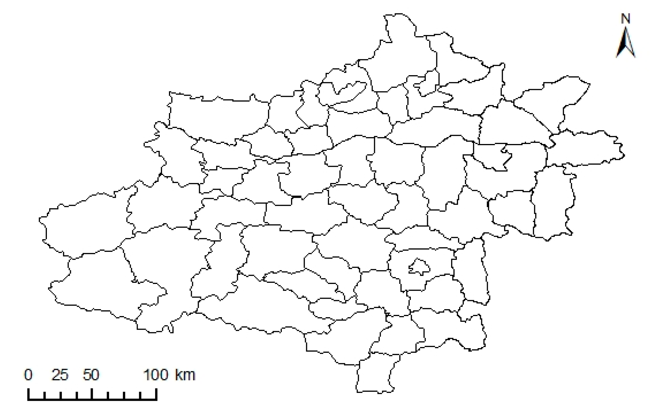
The case study area is based on Zhongyuan urban agglomeration in Henan Province, China. This area includes nine prefecture-level city administrative divisions: Zhengzhou, Kaifeng, Luoyang, Pingdingshan, Xinxiang, Jiaozuo, Luohe, Xuchang, and Jiyuan. We also take county level administrative regions as another set of basic regional units (this includes counties, county-level cities and municipal districts). However, related economic growth data for the smaller municipal districts are not easy to obtain, so districts under the jurisdiction of prefecture-level cities are merged into several ‘urban districts’ when performing the data analysis. After this treatment, the Zhongyuan urban agglomeration of China consists of 56 spatially adjacent urban districts, county-level cities and counties (See Figure 2); they are collectively referred to as “sample regions”.
3.2. Data
This paper selects the years between 1993 and 2009 as the study period. The data used are all obtained from the 1994–2010 editions of the Henan Statistical Yearbook where the main data include population, gross domestic product (GDP), and total fixed investment assets in each of the 56 sample regions. Due to the lack of a specific county-level consumer price index data set, we use the province’s consumer price index to adjust for inflation when calculating GDP of the county districts, and then obtain the real GDP based on comparable prices in 1990. Because there are no related statistical data of capital stock in the Zhongyuan urban agglomeration, the paper uses investment flow data and the perpetual inventory method to obtain estimates of the capital stock data. In the estimation of capital stock, most scholars use the perpetual inventory method, but there are some problems with this method. Because the earlier the base year chosen, the smaller the impact which the error of capital stock estimates will cause in subsequent years [34]. Therefore, the base time of the national capital stock estimation is often chosen as 1952 in China. However, this paper examines the county capital stock, and one cannot obtain that early an estimate of total investment in fixed assets at the county level due to data constraints. Therefore, there may be some disparities between the measured data in this paper and the real capital stock. However, this paper introduces capital stock as an explanatory variable into the model and focuses on it as a basis for further research, rather than focusing on estimating the capital stock itself, so this potential source of error should not have a significant impact on the main conclusions of the article. Kt = (1 − δ) Kt−1 + It, where Kt and It are the respective capital stock and investment for the period t, and δ is a geometric rate of depreciation. The base period capital stock is calculated in accordance with the common method [35]. That is, where K0 = I0/(g + δ),where g is the average annual growth rate of real investment of the sample period, and K0 and I0 are the capital stock and investment in the base period. The depreciation rate is 5%, in accordance with the choice of the majority of Chinese investigators [36,37]. The actual fixed asset investment data are obtained by converting the fixed asset investment price index and are based on constant prices in 1990 yuan. The fixed assets investment price index is replaced by the fixed assets investment in the price index in Henan Province referring to Zhang’s method to account for data missing in the period prior to 1996 [38]. These data for the years 1994, 1995 and 1996 for fixed asset investments are obtained by computing the implicit investment deflator index according to Zhang et al. (2004) [35]. Data after 1996 are available, so we use the fixed assets investment price index published in the China Statistical Yearbook. With regard to the sample regions which have experienced administrative changes in the study period, we base the data on the administrative divisions in 2010.
3.3. Test of the Hypothesis of Spatial Club Convergence
We use the theoretical convergence model of spatial club convergence mentioned above under the assumptions of regional economic homogeneity, and test whether the 56 sample regions of Zhongyuan urban agglomeration were subject to spatial club convergence in the years 1993–2009.We introduce a spatial weight matrix W to Equation (33). Two weight matrix types are adopted: first-order contiguity rook-rule matrix (RW) and per capita GDP based weight matrix (GW). Per capita GDP based weight matrix is expressed as:
where per GDPi represents region i’s per capita GDP [39]. is in a standardized form so Equation (33) can be rewritten as a spatial econometric model in Equation(34):
where α is the constant term, and denotes the per capita GDP growth rate of region i. Due to limitations of data availability, we use the population of each sample region to replace the amount of labor actually available in each sample region. denotes the per capita GDP of region i in the initial year, denotes the per capita capital growth rate of region i, denotes the population growth rate of region i, denotes the per capita capital in the initial year of region i, denotes the population in the initial year of region i, denotes a random error term, and , , , , , and are the respective coefficients to be estimated for the above variables.
Here, the form of the spatial econometric model used is the spatial cross-regressive model. The basic form of the model is as follows in Equation (35):
where and are respective matrixes consisting of two sets of explanatory variables in the model; the difference is that denotes the explanatory variable matrix of observations of the target region, whereas , which is the product of and W, denotes the explanatory variable matrix of average observations of the neighboring regions of the target region. Abreu et al. (2005) states that this form of the model can be used to capture spatial spillover effects and names this kind of model “the spatial cross-regressive model” [15]. The application of this model can avoid over-reliance on the spatial error model and the spatial lag model. This paper will not repeat the basic form of these two universal applied spatial econometric models. This model not only introduces the conventional non-spatial lag explanatory variables but also introduces some average characteristics of the neighboring regions as the explanatory variables of model. The significant difference of this model from other spatial econometric models is that the spatial lag term is exogenous, thus the presence of these variables does not directly lead to biased estimates of the model, so we can use ordinary least squares (OLS) in the estimation. Therefore, we use OLS to estimate Equation (34).
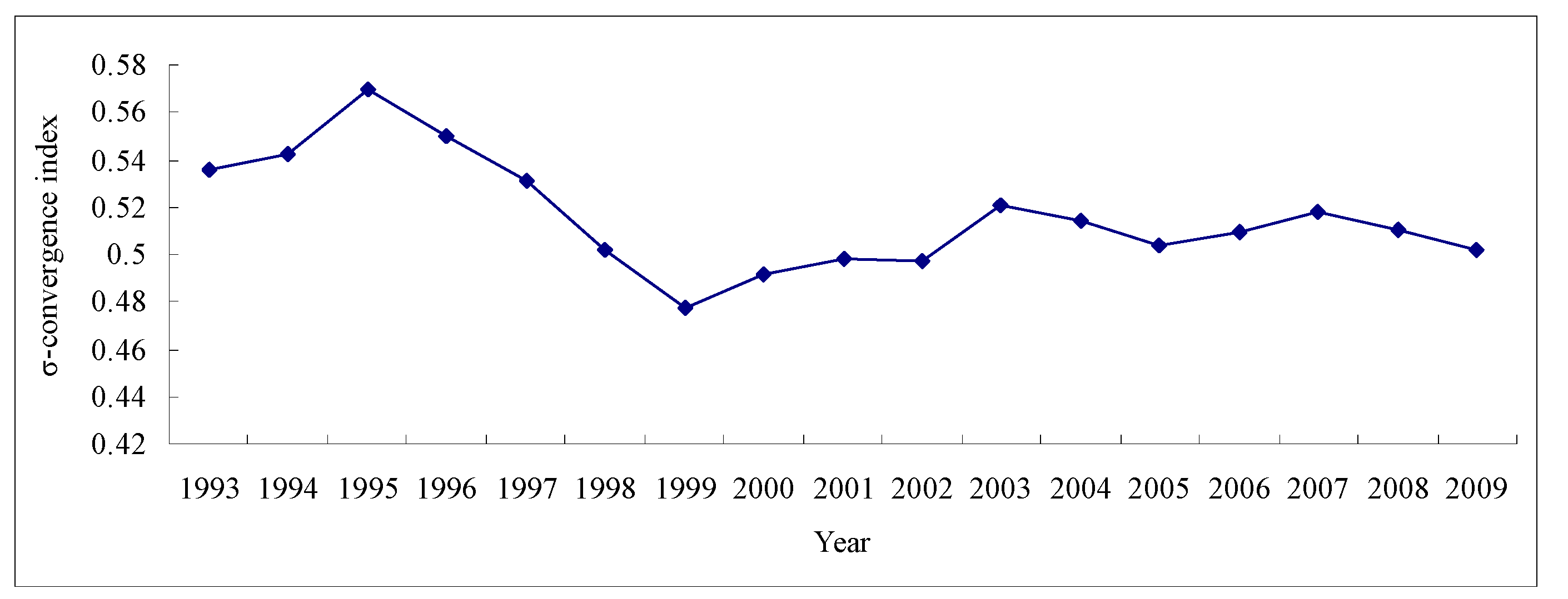
In order to accurately examine the impact of temporal heterogeneity of regional economic growth to the determination of spatial club convergence, we calculate the regional convergence index σ of the Zhongyuan urban agglomeration of China in the period 1993–2009.
σ convergence is measured as:
where yi,t is region i’s measurement at Time t, σt is the standard deviation of observations among n regions. If t + T reaches σt+T < σt, these n economies realize σ convergence at Time T. If any time of s > t shows σs < σt, these n economies have the consistent σ convergence.
The results of this analysis are shown in Figure 3.
According to the calculations of the index of σ convergence, the gap of per capita GDP in 1993–2009 in Zhongyuan urban agglomeration of China has apparent temporal heterogeneity. That is, the income distribution shows different characteristics before and after 1999. Therefore, when estimating the spatial club convergence model, we consider the point 1999 as a time segment, and we estimate the three different periods 1993–2009, 1993–1999, and 2000–2009 respectively to examine if there is spatial club convergence in Zhongyuan urban agglomeration. The estimation results are shown in Table 1.
Based on the estimates summarized in Table 1, we can reach four conclusions as follows.
The first-order contiguity weight matrix is better to describe the spatial spillover than the other weight matrix. It means that location plays a more important role in spatial spillover. Comparing the estimating results of the three periods, the model fit of 1993–1999 is optimal, indicating Zhongyuan urban agglomeration had a significant spatial club convergence in 1993–1999, and the corresponding convergence rate is 2.0%, which is consistent with the empiricalfindingsfor108Europeanregions [40]. For the entire period of 1993–2009, we can also obtain the result that there was significant spatial club convergence, and the convergence rate was 1.0%.
Second, for the significant parameter estimates, the estimated results of φ5 and φ6 in 1993–1999 are highly significant, indicating that the initial population of neighboring regions and initial population in the target region are the most important impact factors for the economic growth rate of the target region. However, the two effects are opposite. That is, larger initial population in neighboring regions will help to improve the per capita GDP growth rate of the target region, but a larger initial population in the target region has a blocking role on its own per capita GDP growth rate. This implies that it is easier for a low population area adjacent to a high population area to grow rapidly. In the estimated results in the 2000–2009 period, φ1、φ2、φ4 and φ6 are significant at different degrees, where φ1、φ2、φ4 respectively reflect capital and population growth rate of neighboring regions, and the impact of initial capital stock on per capita GDP growth rate of the target region. We can see that these three variables all have positive effects on the per capita GDP growth rate of the target region. This indicates that the target region receives positive spatial spillover effects from the capital and population in the neighboring regions, and the spatial spillover effects play an important role in the process of spatial club convergence in Zhongyuan urban agglomeration.
Third, from the perspective of the spatial dependence test of the set model, Moran’s I indicators in the three periods are not significant, which indicate that residuals are not spatially auto-correlated, and ensure that the results of OLS are reliable, after the exogenous spatial lag variables are considered.
Fourth, from the results of the residuals state test (Jarque-Bera method), the 1993–2009 period does not pass the significance test, and the other two periods are significant, indicating that from the point of view of the whole period, there exists significant temporal heterogeneity. Therefore, the selected 1993–2009 period is not suitable for estimation using a single test model.
4. Conclusions
This paper argues that the concept of club convergence of Barro and Sala-i-Martin is limited to the temporal dimension. This classical club convergence model ignores the reality that regional economic growth has a spatial correlation, spatial heterogeneity and spatial agglomeration (clustering). In order to explain the phenomenon of regional clusters in regional economic growth realistically, it is necessary to explore the spatial attributes of club convergence on the basis of club convergence models in both the temporal and spatial dimensions. This in turn requires the creation of a concept of spatial club convergence. This paper proposes and tests the hypothesis of spatial club convergence.
The paper defines spatial club convergence as the situation where a group of regions which are spatially adjacent and have similar initial conditions and structural characteristics will converge to the same steady state of economic growth. By combining the spatial spillover effects present in the new economic geography and the formation mechanism of club convergence in neoclassical growth theory, the paper proposes the mathematical form of the mechanism of spatial club convergence. More specifically, under the conditions of mutual free trade and exchange and the free flow of factors of production, and as a result of the dual role of diminishing marginal returns of factors and spatial spillover effects, a group of regions which are spatially adjacent and have similar initial conditions and structural characteristics will converge to the same steady state. The paper constructs the theoretical model of spatial club convergence based on the Solow model, and theoretically proves the hypothesis of spatial club convergence. In addition, the paper conducts a club convergence test on the regional economic growth of Zhongyuan urban agglomeration of China in the years 1993–2009, and the results show that in the two periods of 1993–1999, and 1993–2009, there was spatial club convergence in the 56 regions of Zhongyuan urban agglomeration of China, the respective convergence rates were 2.0% and 1.0%. Hence, both theoretical deduction and empirical studies verify the hypothesis of spatial club convergence.
Spatial club convergence is an increasingly popular field in the study of regional economic convergence. The paper has proposed and tested the hypothesis of spatial club convergence in inland China. However, there are still limitations in the work. The main issue is that the theoretical model in the paper cannot unconditionally draw the conclusion of spatial club convergence in the case where there are major spatial spillover effects from areas that are not adjacent. On the contrary, spatial club convergence is impacted by a variety of conditional constraints. The condition here is not identical with the condition in conditional convergence; and it mainly emphasis the spatial correlation and temporal heterogeneity in regional economic growth. This is different from the classical Solow model which yields unconditional proof of convergence. Therefore, we must perform a condition test to determine the presence of spatial club convergence. The spatial club convergence condition derived from theoretical model is difficult to directly test with empirical data because we cannot obtain the real data for some of the parameters. However, through the inspection of the growth equation, we can indirectly determine whether there is spatial club convergence in the case area, and present limited discussion of the practical significance of the parameters. Secondly, the paper only presents a general analysis of spatial spillover effects. Hence, only some factors from neighboring regions are considered, and no factors from the focal regions are included. In a subsequent study, the source of spatial spillover effects can be refined, thus analysis of the role of a variety of spatial spillover effects in the spatial club convergence should be performed in-depth. In addition, the inclusion of the focal region’s factors will lead to a more robust outcome. Thirdly, when analyzing the role of spatial spillover effects in spatial club convergence, as a result of the desire to simplify the problem, we treated neighboring regions as homogenous, ignoring the unique “personality” of each neighboring region of each target region, and only discuss the limited differences of the target region and its neighboring regions. In future work, we shall attempt to discuss the spatial spillover effects of neighboring regions under different conditions from the target region and the corresponding dynamic characteristics. The 56 sample regions in Zhongyuan urban agglomeration of China were chosen without regional grouping and selection, which may affect the test results of the hypothesis of spatial club convergence. In addition, more case studies are needed in other areas to perform rigorous empirical testing of the spatial club convergence concept.
Acknowledgments
This work was supported by the National Social Science Foundation of China (No. 11&ZD159) and National Natural Science Foundation of China (41430637; 41329001) and funded by Center for Collaborative Innovation Research on New Urbanization and CPEZ Construction.
Author Contributions
Chenglin Qin and Yingxia Liu co-designed and performed the research. Xinyue Ye provided the method of data analysis and modified the draft. All authors read and approved the final manuscript.
Conflicts of Interest
The authors declare no conflict of interest.
References
- Wei, Y.D.; Ye, X. Beyond Convergence: Space, Scale, and Regional Inequality in China. Tijdschr. Econ. Soc. Geogr. 2009, 100, 59–80. [Google Scholar] [CrossRef]
- Fischer, M.M.; Stirböck, C. Pan-European regional income growth and club-convergence insights from a spatial econometric perspective. Ann. Reg. Sci. 2006, 40, 693–721. [Google Scholar] [CrossRef]
- Ye, X.; Wei, Y.D. Regional Development, Disparities and Polices in Globalizing Asia. Reg. Sci. Policy Pract. 2012, 4, 179–182. [Google Scholar] [CrossRef]
- Postiglione, P.; Andreano, M.S.; Benedetti, R. Using constrained optimization for the identification of convergence clubs. Comput. Econ. 2013, 42, 151–174. [Google Scholar] [CrossRef]
- Lim, U. Regional income club convergence in US BEA economic areas: A spatial switching regression approach. Ann. Reg. Sci. 2016, 56, 273–294. [Google Scholar] [CrossRef]
- Ye, X.; Rey, S.J. A Framework for Exploratory Space-Time Analysis of Economic Data. Ann. Reg. Sci. 2013, 50, 315–339. [Google Scholar] [CrossRef]
- Laurini, M.; Andrade, E.; Valls Pereira, P.L. Income convergence clubs for Brazilian municipalities: A non-parametric analysis. Appl. Econ. 2005, 37, 2099–2118. [Google Scholar] [CrossRef]
- Dall’erba, S.; Le Gallo, J. Regional convergence and the impact of European structural funds over 1989–1999: A spatial econometric analysis. Pap. Reg. Sci. 2008, 87, 219–244. [Google Scholar] [CrossRef]
- Olejnik, A. Using the spatial autoregressively distributed lag model in assessing the regional convergence of per-capita income in the EU25. Pap. Reg. Sci. 2008, 87, 371–384. [Google Scholar] [CrossRef]
- Pfaffermayr, M. Conditional β and σ-convergence in space: A maximum likelihood approach. Reg. Sci. Urban Econ. 2009, 39, 63–78. [Google Scholar] [CrossRef]
- Ye, X.; Yue, W. Comparative Analysis of Regional Development: Exploratory Space-Time Data Analysis and Open Source Implementation. Economics. 2014. Available online: http://www.economics-ejournal.org/economics/discussionpapers/2014-20 (accessed on 25 June 2017).
- Ertur, C.; Koch, W. Growth, technological interdependence and spatial externalities: Theory and evidence. J. Appl. Econom. 2007, 22, 1033–1062. [Google Scholar] [CrossRef]
- Fischer, M.M. A spatial Mankiw-Romer-Weil model: Theory and evidence. Ann. Reg. Sci. 2011, 47, 419–436. [Google Scholar] [CrossRef]
- Liu, Y.X.; Qin, C.L. Research of regional economic growth spatial convergence hypothesis. Econ. Perspect. 2010, 2, 99–103. [Google Scholar]
- Abreu, M.; De Groot, H.L.F.; Florax, R.J.G.M. Space and growth: A survey of empirical evidence and methods. Rég. Dév. 2005, 21, 13–44. [Google Scholar] [CrossRef]
- Li, Y.; Wei, Y.H.D. Multidimensional Inequalities in Health Care Distribution in Provincial China: A Case Study of Henan Province. Tijdschr. Econ. Soc. Geogr. 2014, 105, 91–106. [Google Scholar] [CrossRef]
- Lemoine, F.; Poncet, S.; Ünal, D. Spatial rebalancing and industrial convergence in China. China Econ. Rev. 2015, 34, 39–63. [Google Scholar] [CrossRef]
- Barro, R.J.; Sala-i-Martin, X. Convergence across states and regions. Brook Pap. Econ. Act. 1991, 1991, 107–182. [Google Scholar] [CrossRef]
- Qin, C.L.; Zhang, W.L. Test and factor analysis of the club convergence of regional economic growth in China: Based on the information of regional grouping by CART. Manag. World. 2009, 3, 21–35. [Google Scholar]
- Cheng, J.; Dai, S.; Ye, X. Spatiotemporal heterogeneity of industrial pollution in China. China. Econ. Rev. 2016, 40, 179–191. [Google Scholar] [CrossRef]
- Fujita, M.; Krugman, P.; Venables, A. The Spatial Economy: Cities, Regions, and International Trade; MIT Press: Cambridge, UK, 1999. [Google Scholar]
- Dall’erba, S. Productivity convergence and spatial dependence among Spanish regions. J. Geogr. Syst. 2005, 7, 207–227. [Google Scholar] [CrossRef]
- Qin, C.L.; Tang, Y. Club convergence of regional economic growth in Henan Province. Geogr. Res. 2007, 26, 548–556. [Google Scholar]
- Qin, C.L.; Zhang, W.L. Review of regional economic growth club convergence. Econ. Perspect. 2008, 3, 103–108. [Google Scholar]
- Quah, D. Galton’s fallacy and tests of the convergence hypothesis. Scand. J. Econ. 1993, 95, 427–443. [Google Scholar] [CrossRef]
- Quah, D. Empirics for economic growth and convergence. Eur. Econ. Rev. 1996, 40, 1353–1375. [Google Scholar] [CrossRef]
- Quah, D. Twin peaks: Growth and convergence in models of distribution dynamics. Econ. J. 1996, 106, 1045–1055. [Google Scholar] [CrossRef]
- BernadiniPapalia, R.; Bertarelli, S. Identification and Estimation of Club Convergence Models with Spatial Dependence. Int. J. Urban Reg. Res. 2013, 37, 2094–2115. [Google Scholar] [CrossRef]
- Pan, X.; Liu, Q.; Peng, X. Spatial club convergence of regional energy efficiency in China. Ecol. Indic. 2015, 51, 25–30. [Google Scholar] [CrossRef]
- Rumayya, W.W.; Erlangga, A.L. Club convergence & regional spillovers in East JAVA. Reg. Econ. Dev. 2005, 17, 1315–1445. [Google Scholar]
- Egger, P.; Pfaffermayr, M. Spatial convergence. Pap. Reg. Sci. 2006, 85, 199–215. [Google Scholar] [CrossRef]
- Barro, R.J.; Sala-i-Martin, X. Convergence. J. Polit. Econ. 1992, 100, 223–251. [Google Scholar] [CrossRef]
- Barro, R.J.; Mankiw, N.G.; Sala-i-Martin, X. Capital mobility in neoclassical models of growth. Am. Econ. Rev. 1995, 85, 103–115. [Google Scholar]
- Lei, H. Estimating capital stock and investment efficiency in China. Economist 2009, 9, 75–83. [Google Scholar]
- Zhang, J.; Wu, G.Y.; Zhang, J.P. The estimation of China’s provincial capital stock: 1952–2000. Econ. Res. J. 2004, 39, 35–44. [Google Scholar]
- Wang, X.L.; Fan, G. Sustainability of China’s Economic Growth; Economic Science Press: Beijing, China, 2000. [Google Scholar]
- Guo, Q.W.; Jia, J.X. Estimating total factor productivity in China. Econ. Res. J. 2005, 40, 51–60. [Google Scholar]
- Zhang, X.L. Economic convergence and its effect mechanism in Yangtze River Delta Region: 1993–2006. J. World Econ. 2010, 3, 126–140. [Google Scholar]
- Zhang, Z.Q. Type of spatial Weight on Spatial Panel Parameters estimation and testing efficiency. J. Quant. Tech. Econ. 2014, 10, 122–138. [Google Scholar]
- López-Bazo, E.; Vayá, E.; Manuel, A. Regional externalities and growth: Evidence from European regions. J. Reg. Sci. 2004, 44, 43–73. [Google Scholar] [CrossRef]
Figure 1.
Diagram of the theoretical behavior of illustrates the convergence toward a steady state.
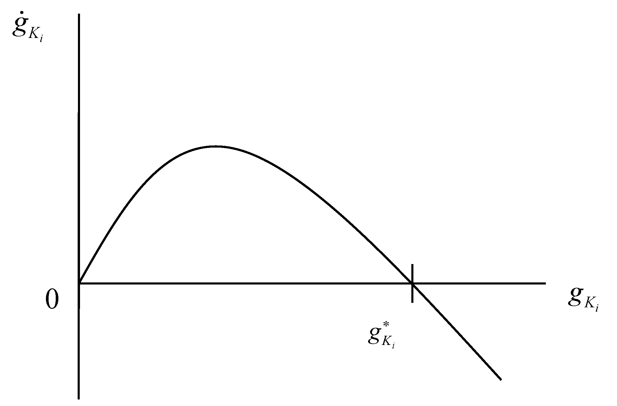
Figure 2.
The 56 sample regions.

Figure 3.
The σ convergence index of Zhongyuan urban agglomeration in 1993–2009.


Table 1.
The OLS estimates of the spatial club convergence model in Zhongyuan urban agglomeration.
| 1993–2009 | 1993–1999 | 2000–2009 | ||||
|---|---|---|---|---|---|---|
| RW | GW | RW | GW | RW | GW | |
| constant | −2.13(−1.12) | −0.14(−1.23) | −0.68(−1.04) | −0.04(−0.23) | 0.33(0.22) | −0.003(−0.02) |
| −0.17(−3.79) *** | 0.02(2.03) ** | −0.15(−3.08) *** | −0.01(0.86) | −0.19(−2.31) ** | 0.009(0.55) | |
| φ1 | 0.44(2.23) ** | −0.008(−0.39) | −0.001(−0.02) | −0.001(−0.07) | 0.28(1.71) * | 0.009(0.10) |
| φ2 | 1.74(1.44) | −0.16(−0.09) | −0.15(−0.08) | −3.12(−0.94) | 2.65(2.61) ** | 1.33(0.80) |
| φ3 | −0.43(−0.86) | −0.81(−1.32) | 0.11(0.14) | −1.09(−1.03) | −0.50(−1.29) | −0.24(−0.39) |
| φ4 | 0.39(2.88) *** | −0.02(−2.53) *** | 0.006(0.12) | −0.002(−0.15) | 0.29(2.61) ** | −0.02(−1.32) |
| φ5 | 0.64(2.98) *** | 0.03(2.77) *** | 0.41(3.33) *** | 0.01(1.07) | 0.19(0.96) | 0.02(0.95) |
| φ6 | −0.05(−0.46) | −0.01(1.18) | −0.18(3.08) *** | −0.001(−0.09) | −0.23(−2.65) ** | 0.01(0.80) |
| R2 | 0.32 | 0.19 | 0.51 | 0.09 | 0.43 | 0.07 |
| F | 4.11 | 1.62 | 7.25 | 0.73 | 4.89 | 0.56 |
| LIK | −8.79 | 127.47 | 24.15 | 103.6 | 1.96 | 103.24 |
| AIC | 33.65 | −238.94 | −32.30 | −191.2 | 12.23 | −190.48 |
| SC | 50.23 | −222.74 | −16.10 | −174.99 | 28.45 | −174.28 |
| Moran’ I | 0.22[0.48] | − | 0.15[0.38] | − | 0.21[0.46] | − |
| Breusch-Pagan | 13.42[0.08] | 4.52[0.71] | 13.50[0.06] | 4.5[0.71] | 13.31[0.07] | 3.77[0.80] |
| Jarque-Bera | 2.19[0.38] | 2.50[0.28] | 7.26[0.03] | 1.15[0.56] | 5.29[0.08] | 26.05[0.00] |
Standard errors in parentheses and p value in square brackets; * means that the significant level at 10%, ** at 5%, and *** at 1%.
© 2017 by the authors. Licensee MDPI, Basel, Switzerland. This article is an open access article distributed under the terms and conditions of the Creative Commons Attribution (CC BY) license (http://creativecommons.org/licenses/by/4.0/).
Share and Cite
MDPI and ACS Style
Qin, C.; Ye, X.; Liu, Y. Spatial Club Convergence of Regional Economic Growth in Inland China. Sustainability 2017, 9, 1189. https://doi.org/10.3390/su9071189
AMA Style
Qin C, Ye X, Liu Y. Spatial Club Convergence of Regional Economic Growth in Inland China. Sustainability. 2017; 9(7):1189. https://doi.org/10.3390/su9071189
Chicago/Turabian StyleQin, Chenglin, Xinyue Ye, and Yingxia Liu. 2017. "Spatial Club Convergence of Regional Economic Growth in Inland China" Sustainability 9, no. 7: 1189. https://doi.org/10.3390/su9071189
Note that from the first issue of 2016, this journal uses article numbers instead of page numbers. See further details here.