A Feedback Control Method for Addressing the Production Scheduling Problem by Considering Energy Consumption and Makespan

Abstract

Due to various factors of uncertainty within production, the key performance indicators connected to production plans are difficult to fulfil. This problem becomes especially serious as emission regulations are enforced, which discourage manufacturers from high emission output and high energy consumption. Thus, this paper proposes a feedback control method for the production scheduling problem by considering energy consumption and makespan to help manufacturers keep production implementations in pace with production plans. The proposed method works in a rolling horizon framework, which establishes planned energy consumption and makespan, and adjusts the weights of the multiple scheduling optimization objectives for the next period, based on the feedback of the actual energy consumption and makespan in previous periods. A job shop scheduling case study is provided to illustrate the proposed method. The experiment results demonstrate the effectiveness of the proposed feedback control method.

1. Introduction

Under the pressure of increasing environmental protection concerns, stricter legislation and rising energy costs, improving energy efficiency in the manufacturing industry has become a critical objective. Meanwhile, the highly competitive market drives manufacturing companies to maintain high levels of productivity by working with traditional production scheduling problems, such as optimizing processing time, cost, etc. As a result, most manufacturing companies are caught in the dual challenge of managing energy consumption (EC) and maintaining production efficiency. At the same time, as information technology, and especially the internet of things (IoT) technology develops and is gradually applied in the manufacturing domain, a lot of detailed information about the manufacturing processes/operations and their relationship with EC becomes available. This enables us to realize energy and production efficient manufacturing by using the low-level manufacturing operation data. In this area, Marzband has completed research [1,2,3,4,5,6,7,8,9,10,11] on algorithms, decision-making methods, control mechanisms, and has contributed an optimal energy management system for smart microgrids. Mourtzis [12,13] studied the cloud-based adaptive process planning and shop-floor scheduling method while considering machine tool status. Fysikopoulos [14,15] made a process planning system for energy efficiency by considering the machine modes. Larreina [16] worked on a smart manufacturing execution system.

However, the challenge that this paper tackles is not solely how to improve the energy and manufacturing efficiency by production planning and scheduling, but it is also concerned with how to make and effectively implement the production plan. Due to the many uncertain factors in production, the key performance indicators within production plans are difficult to fulfill as planned. This leads to a disconnection between production practices and production plans, which makes production plans infeasible as actual production processes deviate from production plans. This problem becomes especially serious as emission regulations are enforced, which limits manufacturers’ emission output and energy consumption.

Thus, this paper proposes a feedback control method for the production scheduling problem by considering energy consumption and makespan, to help manufacturers keep production implementations in pace with production plans. The proposed method works in a rolling horizon framework. A multi-objective optimization model of a job-shop scheduling problem is used to illustrate the feedback control method. In the method, when the actual value of EC exceeds its predicted value, i.e., one of the shop floor’s key performance indicators (KPIs), rescheduling strategies will be activated to modify the production scheduling model parameters of the next period by adjusting the weights of objective functions. Currently, this feedback control scheduling model aims to balance the EC and makespan (MS) by keeping them within the expected boundary, which is an important issue, as more and more manufacturing companies have to face the emission trading scheme (ETS).

The remainder of this paper is organized as follows: Section 2 introduces the contribution of this paper by comparing it with related works. Section 3 presents the feedback control method. The multi-objective optimization model of a job-shop scheduling problem and the corresponding algorithm are provided. Then, a case study is used to validate the proposed method in Section 4. Section 5 presents the conclusion.

2. Related Works

This paper is based on the work from three perspectives as described in the following paragraphs.

The first to consider is an energy-aware manufacturing system. By observations from Japan, Europe and the United States, Gutowski et al. [17] pointed out that environmentally benign manufacturing needed systems level thinking and strategic planning. With a case study at an automotive paint shop, [18] showed that EC could be reduced significantly through production system design. Through interviews with industry representatives, Ernst et al. [19] found there was a need for energy efficiency KPIs to track the changes and improvements on both the processes and at the plant level, and the need for the integration of real-time data and knowledge-embedded processes to manage and optimize the energy efficiency of the production processes. Hesselbach et al. [20] presented an energy oriented simulation model for the planning of manufacturing systems, which emphasized dynamic interactions of different processes and auxiliary equipment. Seliger et al. [21] introduced an EnergyBlocks method for accurate EC prediction and indicated that real-time energy consumption data, in combination with integrated scheduling algorithms, would allow for the automated adaptation of the actual production schedule. Kellens et al. [22] also provided a structured approach for energy and resource efficient manufacturing, and noted the importance of planning and control optimization methods. Similar to the above work, the feedback control method in this paper combines actual production process data with production scheduling to realize energy-ware manufacturing by considering the dynamic interaction of EC KPIs with different production planning levels. Moreover, the proposed method adopts control strategies from a temporal perspective by adjusting short-term schedules according to comparison results of actual shop floor data and planned KPIs to make the schedule implementation coincide with the production plan. This will be more important than ever as the emission trading scheme prevails at the company level [23,24,25,26,27].

The second consideration is the EC calculating model. Seow and Rahimifard, Liu et al. and Prabhu et al. [28,29,30] proposed models for characterizing EC at various levels such as product level, machine level, process level and plant level within manufacturing systems to analyze the spatial and temporal distribution of EC and evaluate the EC of the facilities at the early stages of manufacturing. Kara and Li, Woolley et al. [31,32] presented models to characterize the relationship between EC and manufacturing parameters or process variables. In the light of these works, this paper makes the assumption that the actual shop floor EC is calculated based on the above proposed models. Therefore, this paper does not use the EC calculating model, but focuses on analyzing the actual shop floor EC data together with the corresponding predicated values used in the production schedules for generating production control policies.

The last perspective is the EC-related production scheduling and multi-objective dynamic scheduling. There has been growing interest in EC-related scheduling in recent years. Twomey et al. [33] presented one of the most well-known works, in which operational methods and a multi-objective mathematical programming model were proposed to minimize EC and total work completion time. The following researches have focused on controlling peak load [34,35], minimizing electricity costs by considering time-dependent stratified electricity prices [36,37,38], and reducing overall EC [39,40,41]. The distinction of this paper is that it treats the EC-related scheduling problem not only as a multi-objective one, but also as a dynamic scheduling problem. In the literature about multi-objective dynamic scheduling, Rossi and Dini, Li and Jiang [42,43] considered new task arrival, temporary part unavailability, and temporary machine breakdown as unexpected events, and proposed event-driven approaches. Fattahi and Fallahi, Li et al. [44,45] discussed the balance between efficiency and the stability of dynamic scheduling problems. Shnits [46] emphasized that the decision criteria for the optimization problem should be changed as the system conditions change. Na and Park [47] dealt with a scheduling problem with multi-level job structures and also pointed out that the scheduling is a short-term planning and controlling activity, and could change frequently in accordance with the production shop status. In this study, the feedback control method adopts similar decision support frameworks as those of [46,47,48,49,50]. As in most of the above research, a genetic algorithm is used in this paper to develop a solution for the scheduling problem. However, this paper distinguishes that the objective function parameters for the production schedule problem are adjusted adaptively, and determined periodically based on actual shop floor status and system priority feedback, besides integrating EC as one of the objective functions.

3. The Feedback Control Method

Traditionally, unexpected events such as machine breakdown or new task arrival, are accepted as the major causes for the actual production progress to be inconsistent with the production plan. In fact, the more common reason is that the parameters, such as operation time, used by various algorithms for generating a production plan, are long-term constant statistical values that cannot reflect the volatility of the actual production status. Furthermore, the traditional planning and scheduling process mostly works in a predictive open-loop manner, which increases the contradictions between the actual production implementation and the plan. Therefore, a feedback control method that emphasizes using the real-time manufacturing operation data in a reactive manner with the higher-level KPIs is presented in this section. In the proposed method, the long-term plan is divided into short-term schedules, which allows the subsequent scheduling to take the actual states in the previous schedules and the deviation from the KPIs of the long-term plan into consideration. A new optimization problem is created for each short-term schedule by adjusting the objective function parameters to make the schedule both operational on the shop floor and also satisfy the KPIs of a higher-level plan in the long-term. In this paper, the objective is to minimize production EC and MS.

3.1. Framework of the Feedback Control Method

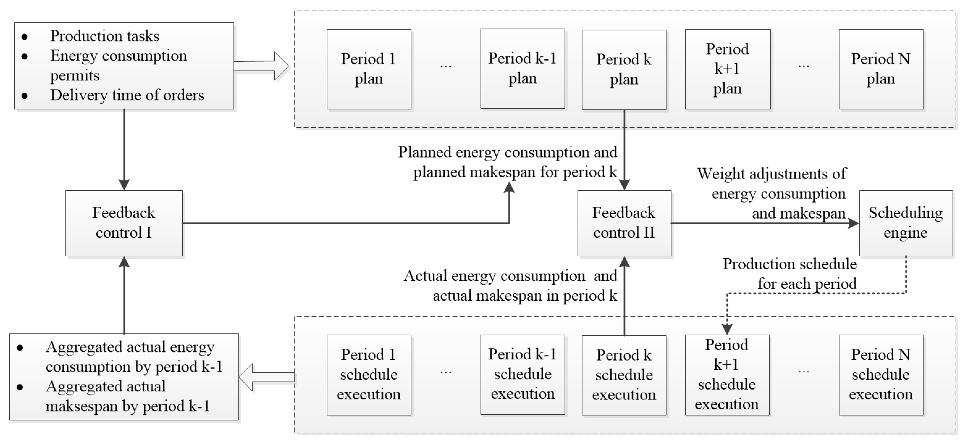
Figure 1 shows the framework of the proposed method. The inputs are the production task, expected EC and delivery time, which can be regarded as the control reference, i.e., requirements from KPIs of the higher-level plan. The outputs include the short-term schedule, and the planned EC and MS for the corresponding production task.

In the proposed method, the long-term production plan horizon is divided into N periods with equal time intervals. The proposed method contains two feedback control functions and a scheduling engine. The first feedback control compares the aggregated actual EC and MS with the permitted EC and the delivery time of orders, and generates the planned EC and MS, i.e., the KPI requirements for the next phase. The second feedback control function adjusts the weights of the optimization objectives in the next period by considering the gap between the planned EC and MS and the actual EC and MS in the previous period. The scheduling engine is used to solve the multi-objective optimization problem for scheduling the production tasks in each period.

3.2. Multiple Objectives

In the feedback control method, two objectives are considered: EC and MS. This multi-objective problem is solved through the combination of the two objectives into a single objective by adding a weighted sum. Thus, the objective function is

$$\min f(w_1,w_2)=w_1{f}_1+w_2{f}_2=w_1\max \{C_1,C_2,\mathrm{...},C_n\}+w_{2}E\hspace{1em}{w}_1+w_2=1;w_1,w_2\ge 0$$

(1)

$f_1$ and $f_2$ represent MS and EC respectively. C_i is the time when job i is finished. E is the total EC. The weights $w_1$ and $w_2$ are fundamental to the result of the solution, and are used to adjust the schedule. If the actual EC is bigger than the planned value, $w_2$ should be increased to strengthen the weight of EC in the next schedule. Similarly, $w_1$should be increased if the actual MS exceeds the planned value.

3.3. Safety Threshold

In order to keep the long-term production plan stabilized, safety thresholds $E_T$ and $T_T$ are introduced in this method. If the deviation between actual value and planned value is within the safety threshold, the previous schedule should be executed within a controllable boundary. Otherwise, the control strategy will be activated to adjust the weights of the scheduling problem for the next stage.

3.4. Production Scheduling Process

The production scheduling process includes the following four steps.

Step 1: The long-term production plan, including both the production task and KPIs of the production plan, is decomposed into N periods. Herein, the KPIs refer to the total EC, i.e., $E_{In}$, and the total MS, i.e., $T_{In}$, in which $E_{In}$ can be taken as the allowed values allocated for this production task. Define $T{a}_i$ as the actual MS in period i, and $E{a}_i$ as the actual EC in period i. Then, the planned MS for sub-tasks in the ith period is

$$T_p^i=(T_{In}-{\displaystyle \sum _{j=0}^{i-1}T{a}_j})/(N-i+1)\hspace{1em}T{a}_j=0;i=1,2,\mathrm{...},N$$

(2)

and the planned EC in the ith period is

$$E_p^i=(E_{In}-{\displaystyle \sum _{j=0}^{i-1}E{a}_j})/(N-i+1)\hspace{1em}E{a}_{j=0}=0;i=1,2,\mathrm{...},N$$

(3)

Step 2: A reactive rolling horizon scheduling mechanism is used to realize production scheduling. In each period, a multi-objective optimization model is applied to determine a satisfactory solution for Equation (1).

Step 3: By comparing the actual MS and EC with the corresponding planned values, the control strategy is used to infer the weights $w_1^{i+1}$ and $w_2^{i+1}$ for the next scheduling period. In this way, a new multi-objective optimization problem is dynamically generated for the next scheduling period based on the actual MS and EC data in the previous periods.

Step 4: Go back to step 2 until period N.

3.5. Control Strategy

The control strategy is as follows. Define

$$\Delta T_i=T{a}_i-T_p^i,\hspace{1em}\Delta E_i=E{a}_i-E_p^i$$

as the deviations of the actual MS and EC from their planned values in the ith period. Then,

(1)

If $\Delta T_i\le T_T$ and $\Delta E_i\le E_T$, the weight is suitable for the actual production, then $w_1^{i+1}=w_1^i$, $w_2^{i+1}=w_2^i$;

(2)

If $\Delta T_i\le T_T$ and $\Delta E_i>E_T$, the actual EC exceeds the safety threshold, but the MS is under control, then, $w_2^{i+1}=w_2^i+k_e\times \Delta E_i$, $w_1^{i+1}=1-w_2^i$;

(3)

If $\Delta T_i>T_T$ and $\Delta E_i\le E_T$, the MS exceeds the safety threshold, but the EC is under control, then $w_1^{i+1}=w_1^i+k_t\times \Delta T_i$, $w_2^{i+1}=1-w_1^i$;

(4)

If $\Delta T_i>T_T$ and $\Delta E_i>E_T$, both the actual MS and EC exceed the safety thresholds, and it requires an analysis of the low-level operation data and the experienced knowledge of workers to infer the weights $w_1^{i+1}$ and $w_2^{i+1}$. The excess may also be caused by the inappropriate allocation of the planned $T_p^i$ and $E_p^i$. In this case, further analysis of the low-level operation data and the experienced knowledge of workers will be necessary.

3.6. The Multi-Objective Optimization Model

The multi-objective optimization model is presented to solve the scheduling problem in each period within the feedback control method. Although the feedback control mechanism can be used for various production scheduling problems, different factories face different types of scheduling problems and will require different models. This paper constructs the model for solving a job-shop scheduling problem by considering the optimisation of both MS and EC.

In the job-shop scheduling problem, there are n kinds of jobs. Each job has m operations, which are processed on m machines respectively, but the process sequences are different. The objective is the minimization of both EC and MS. The assumptions are as follows:

(1)

The processing time of each operation of every job is assumed to be known.

(2)

For each machine, only one job can be processed on it at one time.

(3)

The setup time for each operation is negligible or included in the processing time.

(4)

Each operation should be processed on the specified machine which is known, and only after the current operation is finished, could the next operation begin.

(5)

Job processing cannot overlap.

(6)

Once job processing has begun, it cannot be interrupted.

(7)

The jobs’ processing times on every machine are not deterministic. They are stochastically generated by following the uniform distribution within a possible range.

(8)

The EC for processing, idle, starting up and transportation per unit time can be observed by the monitoring system.

The model of the multi-objective optimization problem is as follows:

$$\min f_1=\max \left\{C_i\right\}\hspace{1em}i=1,2,\mathrm{...},n;$$

(4)

$$\min f_2=E$$

(5)

Subject to:

$$C_i=\max \left\{C_{i,k}\right\}\hspace{1em}i=1,2,\mathrm{...},n;\hspace{1em}k=1,2,\mathrm{...},m;$$

(6)

$$E={\displaystyle \sum _{i=1}^n}{\displaystyle \sum _{k=1}^m{P}_{i,k}}\times Ep{p}_{i,k}+{\displaystyle \sum _{k=1}^m{t}_k}\times Es{p}_k+{\displaystyle \sum _{h=1}^n}{\displaystyle \sum _{k=1}^{m}t{l}_{h,k}}\times Ei{p}_k+{\displaystyle \sum _{i=1}^n}{\displaystyle \sum _{o_i=1}^{m-1}{d}_{o_i{(o+1)}_i}}\times Et{p}_i$$

(7)

$$C_{i,k}-p_{i,k}+M(1-{\alpha }_{i,h,k})\ge C_{i,h}\hspace{1em}i=1,2,\dots n;\hspace{1em}h,k=1,2,\dots m$$

(8)

$$C_{i,k}-C_{i,k}+M(1-x_{i,h,k})\ge p_{i,h}\hspace{1em}i,j=1,2,\dots n;\hspace{1em}k=1,2,\dots m$$

(9)

$$C_{i,k}=p_{i,k}+S_{i,k}\hspace{1em}i=1,2,\dots n;\hspace{1em}k=1,2,\dots m$$

(10)

$$t{l}_{h,k}=S_{{(h+1)}_k,k}-C_{h_k,k}\hspace{1em}{h}_k=1,2,\dots n; k=1,2,\dots m$$

(11)

$$x_{i,j,k}=0or 1 i,j=1,2,\dots n; k=1,2,\dots m$$

(12)

$${\alpha }_{i,j,k}=0 or 1 i=1,2,\dots n; h,k=1,2,\dots m$$

(13)

$C_i$ is the time when job i is finished. E is the total EC. M is a given, large positive number. n is the number of jobs for processing. m is the number of machines. $p_{i,k}$ is the processing time of job i on machine k. $S_{i,k}$ is the time when job i starts to be processed on machine k. $C_{i,k}$ is the time when job i is finished on machine k. ${\alpha }_{i,h,k}$ is defined as: if job i is processed on machine h earlier than machine k, ${\alpha }_{i,h,k}=1$; otherwise, ${\alpha }_{i,h,k}=0$. $x_{i,j,k}$ is defined as: if job i is processed on machine k earlier than job j, $x_{i,j,k}=1$; otherwise, $x_{i,j,k}=0$. $Ep{p}_{i,k}$ is the processing EC per unit time of job i on machine k. $Es{p}_k$ is the starting up EC on machine k, and $t_k$ is the starting up times of machine k. $Ei{p}_k$ is the idle EC per unit time on machine k, and $t{l}_{h,k}$ is the idle time of machine k after job h is finished. $h_k$ means that the job h is processed on machine k. $Etp$ is the transporting EC per unit distance, and $d_{h,k}$ is the distance from machine h to machine k.

There are two optimization objectives: Equation (4) means to minimize the MS, and Equation (5) means to minimize the total EC. Equation (7) is for calculating the total EC, which is the sum of the total processing energy, the total starting up energy, the total idle energy and the total energy for transportation. Equation (6) means that the finished time of a job is equal to the maximized completion time of all of its operations. Equation (8) means that a job’s next operation cannot be processed until its current operation is finished. Equation (9) means that a machine can process a new job only after it has finished the current one. Equation (10) means that the completion time of job i on machine k is equal to the sum of the starting time and the processing time. Equation (11) means that a machine’s idle time is determined by the starting time of the next job and the finishing time of the current job. Both $x_{i,j,k}$ and ${\alpha }_{i,h,k}$ are 0–1 variables. Equation (12) means that if job i is processed on machine k earlier than job j, then $x_{i,j,k}=1$; otherwise, $x_{i,j,k}=0$. Equation (13) means that if job i is processed on machine h earlier than on machine k, then ${\alpha }_{i,h,k}=1$; otherwise, ${\alpha }_{i,h,k}=0$. As explained in Section 2, a genetic algorithm is used to solve the multi-objective optimization problem.

4. Case Study

A job-shop scheduling problem is provided as a case study to validate the feedback control method from three perspectives: effects of the weights in the multi-objective optimization model, the feedback control mechanism, and the safety thresholds.

4.1. Effect of the Weights

The weights are the control variables in each period of the feedback control method, which adjust the trade-off between EC and MS in the multi-objective optimization model. In this case study, only idle machine EC is considered for simplifying the calculation, and different problem sizes are discussed for testing the effects of the weights.

Table 1. Processing time (minutes).

4 Jobs
	M1	M2	M3	M4
J1	22	45	38	47
J2	72	45	58	27
J3	74	71	65	43
J4	36	41	43	59
6 Jobs
	M1	M2	M3	M4	M5	M6
J1	22	45	38	47	29	59
J2	72	45	58	27	35	65
J3	74	71	65	43	41	53
J4	36	41	43	59	59	69
J5	62	49	67	70	56	36
J6	58	64	37	38	57	56
8 Jobs
	M1	M2	M3	M4	M5	M6	M7	M8
J1	22	45	38	47	29	59	46	39
J2	72	45	58	27	35	65	72	47
J3	74	71	65	43	41	53	69	28
J4	36	41	43	59	59	69	44	59
J5	62	49	67	70	56	36	21	69
J6	58	64	37	38	57	56	27	59
J7	33	67	50	55	56	61	22	67
J8	59	60	49	62	37	21	30	66

,

Table 2. Idle energy consumption (EC) (KJ per minute).

4 Jobs
	M1	M2	M3	M4
EC	11	28	23	30
6 Jobs
	M1	M2	M3	M4	M5	M6
EC	11	28	23	30	16	38
8 Jobs
	M1	M2	M3	M4	M5	M6	M7	M8
EC	11	28	23	30	16	38	29	24

and

Table 3. Machine processing sequence.

4 Jobs
	O1	O2	O3	O4
J1	M1	M4	M3	M2
J2	M2	M3	M1	M4
J3	M4	M1	M3	M2
J4	M3	M1	M2	M4
6 Jobs
	O1	O2	O3	O4	O5	O
J1	M1	M4	M3	M2	M6	M5
J2	M4	M5	M1	M2	M3	M6
J3	M6	M1	M3	M2	M5	M4
J4	M3	M1	M2	M4	M5	M6
J5	M6	M5	M1	M3	M2	M4
J6	M5	M1	M6	M2	M3	M4
8 Jobs
	O1	O2	O3	O4	O5	O6	O7	O8
J1	M1	M4	M3	M2	M6	M7	M5	M8
J2	M4	M5	M8	M2	M3	M6	M7	M1
J3	M6	M7	M3	M2	M5	M8	M1	M4
J4	M3	M1	M2	M7	M8	M6	M4	M5
J5	M6	M5	M1	M8	M7	M4	M3	M2
J6	M7	M1	M6	M8	M3	M4	M5	M2
J7	M8	M3	M2	M6	M7	M5	M1	M4
J8	M4	M3	M7	M8	M2	M5	M1	M6

present the processing time, the idle EC of the machines, and the machine processing sequence of the job–shop scheduling problem with different sizes, respectively.

Table 4. Optimization results under different weights.

4 Jobs
No.	$w_1$	$w_2$	$f_1$	$f_2$	$f$	No.	$w_1$	$w_2$	$f_1$	$f_2$	$f$
1	1	0	289	5269	289	13	0.93	0.074	289	5269	658.676
2	0.995	0.056	289	5269	582.619	14	0.92	0.08	289	5269	687.4
3	0.99	0.004	289	5269	307.186	15	0.91	0.088	289	5269	726.662
4	0.985	0.01	289	5269	337.355	16	0.9	0.11	289	5269	839.69
5	0.98	0.13	289	5269	968.19	17	0.85	0.118	289	5269	867.392
6	0.975	0.064	289	5269	618.991	18	0.8	0.124	289	5269	884.556
7	0.97	0.028	289	5269	427.862	19	0.75	0.15	289	5269	1007.1
8	0.965	0.044	289	5269	510.721	20	0.7	0.165	289	5269	1071.685
9	0.96	0.084	289	5269	720.036	21	0.65	0.26	289	5269	1557.79
10	0.955	0.072	289	5269	655.363	22	0.6	0.4	289	5269	2281
11	0.95	0.036	289	5269	464.234	23	0.5	0.5	289	5269	2779
12	0.94	0.024	289	5269	398.116	24	0	1	289	5269	5269
6 Jobs
No.	$w_1$	$w_2$	$f_1$	$f_2$	$f$	No.	$w_1$	$w_2$	$f_1$	$f_2$	$f$
1	1	0	515	19145	515	13	0.97	0.03	562	16908	1796.332
2	0.999	0.001	515	18681	1560.621	14	0.96	0.04	562	16908	1892.16
3	0.998	0.002	515	18681	588.694	15	0.95	0.05	557	17370	2036.544
4	0.997	0.003	521	18819	707.627	16	0.9	0.1	562	16908	2360.06
5	0.996	0.004	515	18681	2941.47	17	0.88	0.12	562	16908	2490.828
6	0.995	0.005	515	18681	1708.009	18	0.87	0.13	562	16908	2588.904
7	0.994	0.006	552	16955	1023.428	19	0.85	0.15	562	16908	3013.9
8	0.993	0.007	515	18681	1333.359	20	0.83	0.17	562	16908	3259.09
9	0.992	0.008	529	18676	2093.552	21	0.7	0.3	562	16908	4811.96
10	0.991	0.009	529	18676	1868.911	22	0.6	0.4	562	16908	7100.4
11	0.99	0.01	557	17370	1176.75	23	0.5	0.5	562	16908	8735
12	0.98	0.02	557	17370	962.74	24	0	1	562	16908	16908
8 Jobs
No.	$w_1$	$w_2$	$f_1$	$f_2$	$f$	No.	$w_1$	$w_2$	$f_1$	$f_2$	$f$
1	1	0	636	27059	636	13	0.96	0.04	659	24611	1096.34
2	0.998	0.002	638	26339	662.423	14	0.95	0.05	664	25226	1616.56
3	0.996	0.004	641	26342	688.846	15	0.94	0.06	661	24550	1967.02
4	0.994	0.006	645	26751	718.103	16	0.92	0.08	673	22929	2402.36
5	0.992	0.008	638	26339	749.424	17	0.91	0.09	660	26391	2966.62
6	0.99	0.01	650	23803	740.804	18	0.85	0.15	660	26012	2837.7
7	0.988	0.012	650	23803	765.765	19	0.8	0.2	661	23210	5014.4
8	0.986	0.014	653	26782	788.918	20	0.75	0.25	661	23331	7191.1
9	0.984	0.016	655	23075	835.903	21	0.7	0.3	661	22549	9367.8
10	0.982	0.018	655	23075	834.36	22	0.6	0.4	661	22428	11544.5
11	0.98	0.02	655	23075	856.78	23	0.5	0.5	661	22428	15897.9
12	0.97	0.03	661	22428	878.67	24	0	1	661	22428	22428

shows the objective function results $f_1$ and $f_2$ of the multi-objective optimization model, i.e., the MS and EC values of the job-shop scheduling problem with the sizes of 4, 6, and 8, under different weights. When the size is 4, the MS and EC values keep invariant despite drastic changes of their weights. When the size is 6 and 8, decreasing tendencies can be observed in both MS and EC as their corresponding weights $w_1$ and $w_2$ increase. The explanation for this is that there are fewer combinations of the job sequences when the size is small, e.g., 4, while there are more combinations of the job sequences when the size gets bigger, e.g., 6 or 8. In other words, there is increased adjustment space as the problem size increases. This may indicate that the weight adjustment has stronger effects on a bigger sized problem.

Moreover, in Table 4, neither MS nor EC monotonically decrease along with increasing $w_1$ or $w_2$, although decreasing patterns can be found between MS, EC and their weights. This is due to the genetic algorithm used in the multi-objective optimization model. Genetic algorithm is a search heuristic that may have a tendency to converge towards local optima, or even arbitrary points, rather than the global optimum of the problem. Nevertheless, the results can testify to the role of weight adjustment in the proposed feedback control method. Future work will be focused on finding new optimization algorithms that are more apt to rebalance multiple objectives by weight adjustment.

4.2. Effect of the Feedback Control Mechanism

The effect of the feedback control mechanism is tested by comparing it with scheduling results without feedback in respect to the deviation of MS and EC from their expected values. The size 8 problem in Table 4 is used here.

The assumption of the problem is described as follows. The expected MS and the EC permit of the long-term plan are 6500 and 250,000 respectively. The long-term plan is divided into ten scheduling periods. Therefore, the expected MS and EC values for each period are: MS_e = 650 and EC_e = 25,000. In each period, the actual MS and EC are generated from normal distributions: MS_a is from $N(M{S}_s,7)$, EC_a is from $N(E{C}_s,2000)$, in which MS_s and EC_s are the $f_1$ and $f_2$ of the selected scheduling solution, as shown in Table 4. This means that even though there is no unexpected event, the actual data may still deviate from those in the selected scheduling solution due to the variability of the parameters in practical implementation. The quality of the scheduling results is measured by the accumulative deviation of MS and EC from their expected values, which are calculated by:

$$\Delta MS={\displaystyle \sum _{i=1}^n\left(M{S}_{e,i}-M{S}_{a,i}\right), n \mathrm{is} \mathrm{the} \mathrm{period} \mathrm{number}}$$

(14)

$$\Delta EC={\displaystyle \sum _{i=1}^n\left(E{C}_{e,i}-E{C}_{a,i}\right), n \mathrm{is} \mathrm{the} \mathrm{period} \mathrm{number}}$$

(15)

As shown in

Table 5. Comparison between the traditional scheduling method and the feedback control scheduling method.

Traditional Scheduling Method
Period No.	Actual Data		Scheduling Plan and Planned MS, EC			Accumulative Deviation with Expected Value
	MSa	ECa	No.	MSp	ECp	∆MS	∆EC
1	654.3037	23,643.074	7	650	25,000	−4.3037	1356.926
2	652.9354	23,860.521	7	650	25,000	−7.2390	2496.405
3	648.0338	25,315.787	7	650	25,000	−5.2728	2180.618
4	644.9283	22,434.408	7	650	25,000	−0.2012	4746.210
5	655.4449	23,214.082	7	650	25,000	−5.6461	6532.128
6	653.3379	24,842.227	7	650	25,000	−8.9840	6689.901
7	648.7398	22,143.234	7	650	25,000	−7.7238	9546.667
8	656.0027	23,094.805	7	650	25,000	−13.7266	11,451.862
9	650.7913	24,064.828	7	650	25,000	−14.5179	12,387.034
10	656.7875	22,462.283	7	650	25,000	−21.3054	14,924.751
The total deviations: ∆MS = Index − Actual = −21.31; ∆EC = Index – Actual = 14,925
Feedback Control Scheduling Method
Period No.	Actual Data		Scheduling Plan and Planned MS, EC			Accumulative Deviation with Expected Value
	MSa	ECa	No.	MSp	ECp	∆MS	∆EC
1	654.3037	23,643.074	7	650	25,000	−4.3037	1356.926
2	639.2677	26,424.922	5	649	25,150	6.4287	–67.996
3	652.2067	23,837.922	6	651	24,991	4.2219	1094.082
4	655.5632	24,989.480	6	651	25,156	–1.3413	1104.602
5	635.5636	26,633.080	5	650	25,184	13.0951	–528.478
6	654.2048	23,396.280	6	653	24,894	8.8903	1075.242
7	652.8790	23,794.967	6	652	25,269	6.0113	2280.275
8	654.1343	23,332.523	6	652	25,760	1.8770	3947.752
9	655.3791	23,549.288	6	651	26,974	−3.5021	5398.464
10	639.9936	27,176.507	5	646	30,399	6.5043	3221.957
The total deviations: ∆MS = Index – Actual = 6.5; ∆EC = Index − Actual = 3221

, while scheduling without feedback, the planned MS and EC in each period are: MS_p = MS_e = 650 and EC_p = EC_e = 25,000. From Table 4, the MS and EC values of scheduling solution No.7 or 6, whose $f_1$ = 650, and $f_2$ = 23,903, are closest to the planned ones. Herein, No.7 scheduling solution is selected to be executed in each period. The total accumulative deviations of MS and EC in the long-term are: ∆MS_t = −21.31 and ∆EC_t = 14,925.

While scheduling with feedback, the planned MS and EC are calculated by Equations (2) and (3) in Section 3.4. If the safety thresholds for MS and EC are: MST = 4, ECT = 1000, then the control strategy in Section 3.5 works as follows. In the 1st period, since $M{S}_p^1$ = 650, $E{C}_p^1$ = 25,000, scheduling solution No.7 is selected. The actual data of No.7 execution is: $M{S}_{a,1}^{}$ = 654.3037, $E{C}_{a,1}^{}$ = 23,643.074. The deviations are: $\Delta M{S}_1^{}$ = 4.3037 > MST, $\Delta E{C}_1^{}$ = −1356.926 < ECT. Thus, $w_1^2$ should be increased, and the control strategy searches the scheduling solution with bigger $w_1^{}$ from the current solution used in Table 4. Because neither MS ($f_1$) nor EC ($f_2$) monotonically decrease along with increasing $w_1$ or $w_2$, the control strategy also compares the scheduling solutions to the planned MS or EC to decide which scheduling solution should be selected. The selection rules are: (1) If $w_1^{i+1}$ should be increased, then the nearest solution with bigger $w_1$ and whose $f_1$ is smaller than $M{S}_p^{i+1}$ should be selected for the $i+1$ period. (2) If $w_2^{i+1}$ should be increased, then the nearest solution with bigger $w_2$ and whose $f_2$ is smaller than $E{C}_p^{i+1}$ should be selected for the $i+1$ period. Therefore, No.5 solution is selected for the 2nd period. In the same way, scheduling solutions for the rest periods are determined as shown in Table 5. The total accumulative deviations of MS and EC in the long-term are: ∆MS_f = 6.5 and ∆EC_f = 3221.

Therefore, the total accumulative deviations of MS and EC with the feedback control mechanism are much smaller than those without it. This proves that the feedback control method can reduce the contradictions in the actual implementation in the long-term plan by making periodic adjustments based on the analysis of actual low-level data. Thus, it is suitable for solving the production scheduling problem. However, it continues to be difficult to choose an ideal solution from the algorithm results for balancing the trade-off among multiple optimization objectives by considering the changeable real-time information in each period. A human–system interaction based method for solving this problem will be a future focus.

4.3. Discussion of the Safety Thresholds

The safety thresholds determine the sensitivity of the feedback control mechanism. If the thresholds are quite small, the feedback control mechanism would be very sensitive. In this case, the resulting frequent schedule changes would be unfavorable to the reality of production, because frequent changes would increase preparation and the workers’ adaptation. On the other hand, if the thresholds are big, the feedback mechanism would not work efficiently to control the actual deviation from the planned indicators. In future work, data mining methods will be studied to establish proper safety thresholds by analyzing historical production data from concrete factories.

5. Conclusions

This paper proposed a feedback control method for scheduling problems to bridge the gap between long-term, higher-level planning, and lower-level shop floor manufacturing implementation. The key is to dynamically adjust the optimization model parameters based on comparing the actual implementation data with the planned manufacturing performance indicators. This paper further considered EC in applying the feedback control method when realizing energy-aware manufacturing. As more and more countries adopt the emissions trading permit policy to combat environmental problems, the proposed feedback control method will be especially suitable for companies in coping with emission trading.

A case study of a job-shop scheduling problem validated the proposed method. The experiment results in Section 4.1 show that the proposed method has a better performance on a larger problem, because a smaller sized problem has narrower adjustment space. It has also been learned that the algorithm used in the scheduling engine may influence the performance of the feedback control method. Therefore, one future focus will be on finding new optimization algorithms that are more apt to rebalance multiple objectives by weight adjustment. By comparing the feedback control method with the traditional method that excludes feedback, the experiment in Section 4.2 proves the effectiveness of the proposed feedback control method. However, how to properly establish the safety thresholds in the feedback control mechanism is still a challenge to be investigated. Another research objective for the future will be connected to the data mining methods for setting proper safety thresholds by analyzing historical production data.

The limitation of this paper is that it only presents the method of how to tune the optimization model parameters, but has not given a detailed parameter optimization method. Therefore, future work will focus on a human–system interaction based method to balance multiple optimization objectives, and data mining methods of historical manufacturing data for the optimized establishment of how to trigger the feedback control.

References

- Marzband, M.; Moghaddam, M.M.; Akorede, M.F.; Khomeyrani, G. Adaptive load shedding scheme for frequency stability enhancement in microgrids. Electr. Power Syst. Res. 2016, 140, 78–86. [Google Scholar] [CrossRef]
- Marzband, M.; Ghazimirsaeid, S.S.; Uppal, H.; Fernando, T. A real-time evaluation of energy management systems for smart hybrid home microgrids. Electr. Power Syst. Res. 2017, 143, 624–633. [Google Scholar] [CrossRef]
- Marzband, M.; Azarinejadian, F.; Savaghebi, M.; Guerrero, J.M. An optimal energy management system for islanded microgrids based on multiperiod artificial bee colony combined with Markov chain. IEEE Syst. J. 2017, 99, 1–11. [Google Scholar] [CrossRef]
- Marzband, M.; Ardeshiri, R.R.; Moafi, M.; Uppal, H. Distributed generation for economic benefit maximization through coalition formation–based game theory concept. Int. Trans. Electr. Energy Syst. 2017, 27, 1–16. [Google Scholar] [CrossRef]
- Marzband, M.; Parhizi, N.; Savaghebi, M.; Guerrero, J.M. Distributed smart decision-making for a multimicrogrid system based on a hierarchical interactive architecture. IEEE Trans. Energy Convers. 2016, 31, 637–648. [Google Scholar] [CrossRef]
- Marzband, M.; Sumper, A.; Ruiz-Álvarez, A.; Domínguez-García, J.L.; Tomoiagă, B. Experimental evaluation of a real time energy management system for stand-alone microgrids in day-ahead markets. Appl. Energy 2013, 106, 365–376. [Google Scholar] [CrossRef]
- Marzband, M.; Sumper, A.; Domínguez-García, J.L.; Gumara-Ferret, R. Experimental validation of a real time energy management system for microgrids in islanded mode using a local day-ahead electricity market and MINLP. Energy Convers. Manag. 2013, 76, 314–322. [Google Scholar] [CrossRef]
- Marzband, M.; Ghadimi, M.; Sumper, A.; Domínguez-García, J.L. Experimental validation of a real-time energy management system using multi-period gravitational search algorithm for microgrids in islanded mode. Appl. Energy 2014, 128, 164–174. [Google Scholar] [CrossRef]
- Marzband, M.; Javadi, M.; Domínguez-García, J.L.; Moghaddam, M.M. Non-cooperative game theory based energy management systems for energy district in the retail market considering DER uncertainties. IET Gener. Transm. Distrib. 2016, 10, 2999–3009. [Google Scholar] [CrossRef]
- Marzband, M.; Parhizi, N.; Adabi, J. Optimal energy management for stand-alone microgrids based on multi-period imperialist competition algorithm considering uncertainties: Experimental validation. Int. Trans. Electr. Energy Syst. 2016, 26, 1358–1372. [Google Scholar] [CrossRef]
- Marzband, M.; Yousefnejad, E.; Sumper, A.; Domínguez-García, J.L. Real time experimental implementation of optimum energy management system in standalone Microgrid by using multi-layer ant colony optimization. Int. J. Electr. Power 2016, 75, 265–274. [Google Scholar] [CrossRef]
- Mourtzis, D.; Vlachou, E.; Doukas, M.; Kanakis, N.; Xanthopoulos, N.; Koutoupes, A. Cloud-based adaptive shop-floor scheduling considering machine tool availability. In Proceedings of the ASME 2015 International Mechanical Engineering Congress & Exposition, Houston, TX, USA, 13–19 November 2015. [Google Scholar]
- Mourtzis, D.; Vlachou, E.; Xanthopoulos, N.; Givehchi, M.; Wang, L. Cloud-based adaptive process planning considering availability and capabilities of machine tools. J. Manuf. Syst. 2016, 39, 1–8. [Google Scholar] [CrossRef]
- Fysikopoulos, A.; Stavropoulos, P.; Papacharalampopoulos, A.; Calefati, P.; Chryssolouris, G. A process planning system for energy efficiency. In Proceedings of the 14th International Conference on Modern Information Technology in the Innovation Processes of the Industrial Enterprises, Budapest, Hungary, 24–26 October 2012. [Google Scholar]
- Fysikopoulos, A.; Pastras, G.; Vlachou, A.; Chryssolouris, G. An approach to increase energy efficiency using shutdown and standby machine modes. In Advances in Production Management Systems. Innovative and Knowledge-Based Production Management in a Global-Local World, Proceedings of the APMS 2014: IFIP Advances in Information and Communication Technology, Ajaccio, France, 20–24 September 2014; Grabot, B., Vallespir, B., Gomes, S., Bouras, A., Kiritsis, D., Eds.; Springer: Berlin/Heidelberg, Germany, 2014; Volume 439, pp. 205–212. [Google Scholar]
- Larreina, J.; Gontarz, A.; Giannoulis, C.; Nguyen, V.K.; Stavropoulos, P.; Sinceri, B. Smart manufacturing execution system (SMES): The possibilities of evaluating the sustainability of a production process. In Proceedings of the 11th Global Conference on Sustainable Manufacturing, Berlin, Germany, 23–25 September 2013; pp. 517–522. [Google Scholar]
- Gutowski, T.; Murphy, C.; Allen, D.; Bauer, D.; Bras, B.; Piwonka, T.; Sheng, P.; Sutherland, J.; Thurston, D.; Wolff, E. Environmentally benign manufacturing: Observations from Japan, Europe and the United States. J. Clean. Prod. 2005, 13, 1–17. [Google Scholar] [CrossRef]
- Guerrero, C.A.; Wang, J.; Li, J.; Arinez, J.; Biller, S.; Huang, N.; Xiao, G. Production system design to achieve energy savings in an automotive paint shop. Int. J. Prod. Res. 2011, 49, 6769–6785. [Google Scholar] [CrossRef]
- Bunse, K.; Vodicka, M.; Schönsleben, P.; Brülhart, M.; Ernst, F.O. Integrating energy efficiency performance in production management–Gap analysis between industrial needs and scientific literature. J. Clean. Prod. 2011, 19, 667–679. [Google Scholar] [CrossRef]
- Herrmann, C.; Thiede, S.; Kara, S.; Hesselbach, J. Energy oriented simulation of manufacturing systems–Concept and application. CIRP Ann. Manuf. Technol. 2011, 60, 45–48. [Google Scholar] [CrossRef]
- Weinert, N.; Chiotellis, S.; Seliger, G. Methodology for planning and operating energy-efficient production systems. CIRP Ann. Manuf. Technol. 2011, 60, 41–44. [Google Scholar] [CrossRef]
- Duflou, J.R.; Sutherland, J.W.; Dornfeld, D.; Herrmann, C.; Jeswiet, J.; Kara, S.; Hauschild, M.; Kellens, K. Towards energy and resource efficient manufacturing: A processes and systems approach. CIRP Ann. Manuf. Technol. 2012, 61, 587–609. [Google Scholar] [CrossRef]
- Du, S.; Zhu, L.; Liang, L.; Ma, F. Emission-dependent supply chain and environment-policy-making in the ‘Cap-and-trade’ system. Energy Policy 2013, 57, 61–67. [Google Scholar] [CrossRef]
- Sun, J.; Wu, J.; Liang, L.; Zhong, R.Y.; Huang, G.Q. Allocation of emission permits using DEA: Centralised and individual points of view. Int. J. Prod. Res. 2014, 52, 419–435. [Google Scholar] [CrossRef]
- Zhang, J.; Zhang, L. Impacts on CO2 emission allowance prices in China: A quantile regression analysis of the Shanghai Emission Trading Scheme. Sustainability 2016, 8, 1195. [Google Scholar] [CrossRef]
- Jiang, W.; Liu, J.; Liu, X. Impact of carbon quota allocation mechanism on emissions trading: An agent-based simulation. Sustainability 2016, 8, 826. [Google Scholar] [CrossRef]
- Ye, B.; Jiang, J.; Miao, L.; Li, J.; Peng, Y. Innovative carbon allowance allocation policy for the Shenzhen emission trading scheme in China. Sustainability 2016, 8, 3. [Google Scholar] [CrossRef]
- Seow, Y.; Rahimifard, S. A framework for modelling energy consumption within manufacturing systems. CIRP J. Manuf. Sci. Technol. 2011, 4, 258–264. [Google Scholar] [CrossRef]
- Li, Y.; He, Y.; Wang, Y.; Yan, P.; Liu, X. A framework for characterising energy consumption of machining manufacturing systems. Int. J. Prod. Res. 2014, 52, 314–325. [Google Scholar] [CrossRef]
- Jeon, H.W.; Taisch, M.; Prabhu, V. Modelling and analysis of energy footprint of manufacturing systems. Int. J. Prod. Res. 2014, 53, 7049–7059. [Google Scholar] [CrossRef]
- Kara, S.; Li, W. Unit process energy consumption models for material removal processes. CIRP Ann. Manuf. Technol. 2011, 60, 37–40. [Google Scholar] [CrossRef]
- Seow, Y.; Rahimifard, S.; Woolley, E. Simulation of energy consumption in the manufacture of a product. Int. J. Comput. Integr. Manuf. 2013, 26, 663–680. [Google Scholar] [CrossRef]
- Mouzon, G.; Yildirim, M.B.; Twomey, J. Operational methods for minimization of energy consumption of manufacturing equipment. Int. J. Prod. Res. 2007, 45, 4247–4271. [Google Scholar] [CrossRef]
- Fang, K.; Uhan, N.; Zhao, F.; Sutherland, J.W. A new approach to scheduling in manufacturing for power consumption and carbon footprint reduction. J. Manuf. Syst. 2011, 30, 234–240. [Google Scholar] [CrossRef]
- Bruzzone, A.A.G.; Anghinolfi, D.; Paolucci, M.; Tonelli, F. Energy-aware scheduling for improving manufacturing process sustainability: A mathematical model for flexible flow shops. CIRP Ann. Manuf. Technol. 2012, 61, 459–462. [Google Scholar] [CrossRef]
- Luo, H.; Du, B.; Huang, G.Q.; Chen, H.; Li, X. Hybrid flow shop scheduling considering machine electricity consumption cost. Int. J. Prod. Econ. 2013, 146, 423–439. [Google Scholar] [CrossRef]
- Moon, J.; Shin, K.; Park, J. Optimization of production scheduling with time-dependent and machine-dependent electricity cost for industrial energy efficiency. Int. J. Adv. Manuf. Technol. 2013, 68, 523–535. [Google Scholar] [CrossRef]
- Moon, J.; Park, J. Smart production scheduling with time-dependent and machine-dependent electricity cost by considering distributed energy resources and energy storage. Int. J. Prod. Res. 2014, 52, 3922–3939. [Google Scholar] [CrossRef]
- Dai, M.; Tang, D.; Giret, A.; Salido, M.A.; Li, W.D. Energy-efficient scheduling for a flexible flow shop using an improved genetic-simulated annealing algorithm. Robot. Comput. Integr. Manuf. 2013, 29, 418–429. [Google Scholar] [CrossRef]
- He, H.; Li, Y.; Wu, T.; Sutherland, J.W. An energy-responsive optimization method for machine tool selection and operation sequence in flexible machining job shops. J. Clean. Prod. 2014, 87, 245–254. [Google Scholar] [CrossRef]
- Pach, C.; Berger, T.; Sallez, Y.; Bonte, T.; Adam, E.; Trentesaux, D. Reactive and energy-aware scheduling of flexible manufacturing systems using potential fields. Comput. Ind. 2014, 65, 434–448. [Google Scholar] [CrossRef]
- Rossi, A.; Dini, G. Dynamic scheduling of FMS using a real-time genetic algorithm. Int. J. Prod. Res. 2000, 38, 1–20. [Google Scholar] [CrossRef]
- Li, L.; Jiang, Z. Self-adaptive dynamic scheduling of virtual production systems. Int. J. Prod. Res. 2007, 45, 1937–1951. [Google Scholar] [CrossRef]
- Fattahi, P.; Fallahi, A. Dynamic scheduling in flexible job shop systems by considering simultaneously efficiency and stability. CIRP J. Manuf. Sci. Technol. 2010, 2, 114–123. [Google Scholar] [CrossRef]
- Zhang, L.; Gao, L.; Li, X. A hybrid genetic algorithm and tabu search for a multiobjective dynamic job shop scheduling problem. Int. J. Prod. Res. 2013, 51, 3516–3531. [Google Scholar] [CrossRef]
- Shnits, B. Multi-criteria optimisation-based dynamic scheduling for controlling FMS. Int. J. Prod. Res. 2012, 50, 6111–6121. [Google Scholar] [CrossRef]
- Na, H.; Park, J. Multi-level job scheduling in a flexible job shop environment. Int. J. Prod. Res. 2014, 52, 3877–3887. [Google Scholar] [CrossRef]
- Keller, F.; Schultz, C.; Braunreuther, S.; Reinhart, G. Enabling energy-flexibility of manufacturing systems through new approaches within production planning and control. Procedia CIRP 2016, 57, 752–757. [Google Scholar] [CrossRef]
- Beier, J.; Thiede, S.; Herrmann, C. Energy flexibility of manufacturing systems for variable renewable energy supply integration: Real-time control method and simulation. J. Clean. Prod. 2017, 141, 648–661. [Google Scholar] [CrossRef]
- Cassettari, L.; Bendato, I.; Mosca, M.; Mosca, R. Energy resources intelligent management using on line real-time simulation: A decision support tool for sustainable manufacturing. Appl. Energy 2017, 190, 841–851. [Google Scholar] [CrossRef]
Figure 1.
Framework of the feedback control method for the production scheduling problem.