Evaluating Urban Forms for Comparison Studies in the Massing Design Stage


1
CENSAM, Singapore-MIT Alliance for Research and Technology, Singapore 138602, Singapore
2
Department of Architecture, Massachusetts Institute of Technology, Cambridge, MA 02139, USA
*
Author to whom correspondence should be addressed.
Sustainability 2017, 9(6), 987; https://doi.org/10.3390/su9060987
Submission received: 11 April 2017
/
Revised: 30 May 2017
/
Accepted: 6 June 2017
/
Published: 8 June 2017
(This article belongs to the Special Issue Sustainable Architecture and Design)
Abstract
:We introduce five performance indicators to facilitate the comparison of urban massing design in the early design stages. The five simple indicators are based on existing studies and cover three main performance areas that are sensitive to urban form changes: solar, ventilation, and connectivity potentials. The first three indicators—the non-solar heated façade to floor area index, daylight façade to floor area index, and photovoltaics envelope to floor area index—measure the solar potential. The frontal area index measures the ventilation potential and the route-directness index measures the connectivity potential. The indicators are simple to use, as they only require urban geometry data for their calculation. We demonstrate the indicators in two case studies; variations in the values of these indicators show that they are sensitive to urban form changes and can be used in comparative studies to identify better performing urban forms among massing designs. We implement the indicators as an open-source Python library, Pyliburo, that designers and researchers can readily access and integrate into their existing design workflows.
1. Introduction
In the early design stages, urban designers compose and manipulate massing models to quickly experiment with different urban forms [1,2,3]. The type of data in a massing model varies depending on the designer and can include building types, architectural typology, land-use, and infrastructure data. We assume that the massing model has the minimal amount of data, which is the geometrical data of the urban form. While this assumption limits design variations in urban form to changes in building form, building layout, and street network, massing models with only geometrical data can still provide quantitative and qualitative feedback for the designers. Quantitatively, the massing models can be computed to provide descriptive information on design aspects such as the density and building heights. Qualitatively, the massing models can be used by the designers to assess aspects such as the visual impact of the building on the surrounding area and the characteristic and shape of the urban spaces. However, it is difficult to compare and identify better design options with only descriptive quantities and a qualitative assessment. Thus, there is a need to measure the performances of the different urban forms to facilitate the comparison and identification of better design options.
We propose the use of performance indicators to facilitate the comparison of different urban forms, as performance indicators are more direct and straightforward to understand than unanalysed results from a performance simulation. Performance indicators are measurable values derived from the results of either simulations or analyses and are used to demonstrate the effectiveness of a design proposal in achieving a performance objective. To enable the comparison of different urban forms with performance indicators, we must first identify the performance areas that will be affected by changes in urban form and then identify the performance indicators from existing studies to aid designers in measuring these performances. We will then customise and automate the calculation of the identified performance indicators for the massing design stage and test the identified performance indicators by applying them in two comparative studies. As the early design stages have many uncertainties, the performance indicators can only measure the potential of a massing design for achieving good performances. We hope that by using the performance indicators, designers are able to choose the massing design with the highest performance potential, so as to maximise these potentials in the later design stage.
The main contribution of this paper is the identification, customisation, and automation of the performance indicators for comparative studies in the massing design stage. There have been similar studies, but the identified performance indicators or simulations in these studies require higher-resolution data than the massing model can provide. Whitford et al. identified four performance indicators to measure the ecological effect of urbanisation. However, the indicators require land cover data for their calculations [4]. Urban Modelling Interface (UMI) is a simulation application that can simulate the solar, energy, and connectivity performance of an urban design [5]. With assumptions about surface materials, UMI’s solar simulation is suitable for assessing solar potentials in the massing design stage. Unfortunately, its energy simulation and connectivity analysis require additional building material and land-use data. We envision that the performance indicators identified in this paper will complement these existing studies by enabling performance evaluation as early as the massing design stage.
2. Method—Identification and Application of the Performance Indicators
In this section, we first identify the performance areas that will be affected by urban form changes. Focusing on these performance areas, we then identify the performance indicators and customise them to measure these performances. The performance indicators will be implemented as a simple-to-use open Python library, Pyliburo, that only requires 3D massing models in the format of Collada [6] or cityGML [7] for the calculations. The calculation will return the indicators and all of the results necessary for visualisation in a Collada format, which can be viewed in various 3D modelling applications. The library will be workflow agnostic and can be easily integrated into an existing design workflow. We will then use the Python library to test the performance indicators in two case studies, showing its feasibility for identifying better design options.
2.1. Performances Affected by Changes in Urban Form
We identified three performance areas that will be affected by urban form changes. Urban form changes in the building form and layout will affect the solar and ventilation performances, as stated in Yang and Chen’s thermal atlas for urban design [8]. Their framework for the thermal atlas is developed based on Oke’s work on urban climate [9]. The effect of building form and layout on solar and ventilation performances is also supported by other studies. Martins et al. used a Simplified Radiosity Algorithm coupled with a Design of Experiment study to determine that closely-packed tall buildings will significantly reduce the amount of solar irradiation falling on the building roof for energy generation in Brazil [10]. Saratsis et al. used a simulation-based daylighting procedure to demonstrate that certain building forms have a better daylighting performance [11]. Ng et al. used wind tunnel analysis and Computational Fluid Dynamics (CFD) simulation in their study to conclude that urban forms are one of the most significant factors affecting urban ventilation in Hong Kong [12]. Srifuengfung used CFD to determine that building orientation and height are the two main factors affecting urban ventilation in Bangkok [13].
Urban form changes in the street network will affect the connectivity potential. Connectivity assesses the effectiveness of the urban form in facilitating the movement of humans and vehicles between destinations. Simulation studies have shown that a street network of high connectivity, a grid-like street pattern with minimal cul-de-sacs, will reduce fuel consumption [14], discourage driving, and encourage walking [15]. Empirical studies have also been conducted to substantiate these claims [16,17]. We have identified three performance areas that will be affected by urban form changes: solar, ventilation, and connectivity performance. Next, we look at the available indicators that can quantify how changes in urban form will affect the three performances.
2.2. Solar Performance Indicators
Solar performance is measured in different ways depending on the climate. For the tropical climate, we want to manipulate the urban forms to shield buildings from solar irradiation to reduce overheating or cooling loads [18,19], while in the temperate climate, we want to maximise solar irradiation falling on the building envelope to be utilised for heating [20]. Regardless of climate, we would want to maximise solar irradiation falling on the building envelope for daylighting [11,21] and energy generation from photovoltaics (PV) [22,23]. Compagnon developed a series of performance indicators to measure an urban design’s potential in utilising solar irradiation for passive heating, PV systems, daylighting, and a solar thermal collector in the temperate climate [20]. First, an irradiation or illuminance threshold value is determined. The threshold value indicates the minimum amount of irradiation or illuminance required for the installation of a solar device. Then, the Radiance lighting simulation [24] is used in the study to simulate the annual cumulative irradiance and illuminance falling on the building envelope. The area of the envelope achieving the threshold value is then normalised by the total building envelope area; the ratio is used to quantify the solar potential of the urban design.
We adopted this approach, but customised the indicator for the tropical climate. For the tropical climate, instead of maximising solar irradiation for heating, we minimised solar irradiation to prevent overheating. As a result, we only used three solar performance indicators for the tropical climate as compared to the four indicators stated in Compagnon’s study. We also improved the indicator by using the total floor area as compared to the total building envelope area for normalisation. By normalising the performance using floor area, we are able to provide a more meaningful ratio for a comparative study, and the façade area achieves a threshold value per floor area. Consider, for example, two massing models with the same density, one with a higher façade area that achieves the threshold value and the other with a lower façade area achieving the threshold value. If the latter has compact building forms with a lower total envelope area, it is possible for the two massing models to have the same result. However, if the floor area is used, the design that has the higher façade area with the threshold value will have a better result. In such cases, designers will be able to differentiate the better performing options more easily with the use of the total floor area.
For calculating the indicators, the GenCumulativeSky module [25] that is distributed with Daysim, is used to simulate the annual cumulative solar irradiance and illuminance distribution on the building massing. We assumed a reflectance value of 0.2 for all building façades, as stated in Compagnon’s study. Once the irradiance or illuminance values are available, they will be analysed according to each indicator.
2.2.1. Non-Solar Heated Façade to Floor Area Index
The Non-Solar Heated Façade to Floor Area Index (NSHFFAI) is the ratio of the façade area receiving an annual solar irradiation equal to or lower than a user-defined threshold value to the net floor area of the urban area (Equation (1)). For a massing design located in the tropical climate, the aim is to maximise the NSHFFAI to reduce the potential of overheating the buildings, thus increasing the likelihood of a lower cooling energy consumption.
where Asolar is the total façade area receiving an annual solar irradiation equal to or lower than a user-defined threshold (m2), and Afloor is the total floor area of the urban area (m2).
NSHFFAI = Asolar/Afloor,
2.2.2. Daylight Facade Area to Floor Area Index
The Daylight Façade to Floor Area Index (DFFAI) is the ratio of the façade area receiving annual mean illuminance equal to or greater than a user-defined threshold value to the net floor area of the urban area (Equation (2)). For a massing design located in the tropical climate, the aim is to maximise the DFFAI to increase the potential of daylighting to reduce the lighting load and energy consumption from lighting in the building.
where Aill is the façade area receiving an annual mean illuminance equal to or greater than a user-defined value.
DFFAI = Aill/Afloor,
2.2.3. Photovoltaic Envelope to Floor Area Index
The Photovoltaic Envelope to Floor Area Index (PVEFAI) is the ratio of the envelope area receiving an annual solar irradiation equal to or greater than a user-defined threshold value to the net floor area of the urban area (Equation (3)). For a massing design located in the tropical climate, the aim is to maximise the PVEFAI to increase the potential of generating enough energy for the building’s energy consumption.
where APVsolar is the envelope area receiving an annual solar irradiation greater than a user-defined threshold value.
PVEFAI = APVsolar/Afloor,
2.3. Ventilation Potential
The major effects of urban forms on urban ventilation are that densely spaced buildings will increase the wind resistance and obstruct the ventilation flow within a neighbourhood. While cities of all climates require ventilation for the removal of polluted air, a different wind speed is preferred, based on different thermal requirements. For example, due to the colder temperature and higher wind speed in many temperate climates, urban areas have narrow winding roads, uniform building heights, and protected city edges to reduce the wind speed in the city [26]. On the other hand, tropical climates have excessive heat and a low wind speed, and thus cities in the tropics will require widely opened streets and outdoor spaces with scattered buildings of varying heights to encourage wind flow in the city [27]. The ventilation flow within a neighbourhood is usually studied in detailed using Computational Fluid Dynamics (CFD) [28] or physical modelling using wind tunnel analysis [29]. These two techniques are complex and time consuming for use in the massing design stage. The Frontal Area Index (FAI) [30,31,32] is an indicator for urban ventilation. FAI indicates the roughness of the urban form; in calculating the FAI, the urban area to be analysed will be gridded, and the FAI is calculated for each grid. FAI is the ratio of the façade area projected to a vertical plane facing a defined wind direction to the area of the occupied grid. A higher FAI indicates an urban form that has a higher potential of obstructing urban ventilation. Wong et al. and Wong and Nichol have modified and used FAI for assessing the ventilation potential of the sub-tropical city of Hong Kong. The modification consists of removing the overlapping façade area projected on the vertical plane. Thus, only the first windward façade is considered in the index, and the subsequently shielded facades are excluded. They have shown in their study that a low FAI is associated with a higher ventilation potential [33,34]. We chose the modified FAI as the performance indicator for measuring the ventilation potential in our study.
Frontal Area Index
For calculating the FAI, we first grid the site and then project the facades onto the vertical plane in the user-defined wind direction. Overlapping surfaces are removed, and the area of the projected surfaces is then calculated and analysed according to Equation (4). A geometrical modelling kernel, PythonOCC, is used for all the geometrical operations. The FAI is calculated for each grid, and the average FAI is used to express the ventilation performance of an urban design. The aim is to minimise the FAI to reduce wind resistance and increase the potential of ventilation through the neighbourhood.
where Afacade is the projected façade area on the vertical plane facing the user-defined wind direction, and Agrid is the area of the grid on which the buildings are located.
FAI = AFacade/Agrid,
2.4. Connectivity Potential
A well-connected street network design means a shorter distance between destinations; the shorter distance will reduce the vehicle travelling time and encourage walking. There are many methods to measure connectivity: to name a few, block size, intersection density, and the link-node ratio [35,36,37]. There is no consensus on a standard measure, but the Leadership in Energy and Environmental Design-Neighbourhood Development (LEED-ND) rating tool uses the intersection density to assess the connectivity of a neighbourhood development. However, Stangl and Guinn have shown that the intersection density can be “gamed” for certain subdivision layouts [38] and Stangl has improved the Route Directness Index (RDI) for a more accurate measure of connectivity [39]. We chose and customised the improved RDI as the performance indicator for measuring the connectivity potential in our study.
Route Directness Index
The Route Directness Index (RDI) is the ratio of the route to straight-line distance between two selected destinations. The aim is to maximise the RDI to produce a more direct route and reduce the travelled distance between destinations. For calculating the RDI, we first extract the geometries of the plots and route network. We then measure the straight-line and route distances between destinations and analyse them according to Equation (5). A geometrical modelling kernel, PythonOCC, is used for all the geometrical operations and a graph theory Python library, Networkx, is used for all route calculations.
where Dstraight is the straight-line distance and DRoute is the route distance.
RDI = DStraight/DRoute,
Originally, the RDI only measured the connectivity between two specific destinations. To measure the connectivity of a neighbourhood, Stangl measured the RDI values of each plot to a set of peripheral points in all directions [39]. The connectivity indicator is then expressed as the ratio of the number of plots that do not have an RDI value lower than the threshold RDI value over the total number of plots. Because we are uncertain about a realistic threshold RDI value for Asian cities like Singapore, we express the connectivity performance of an urban design by calculating the average of the minimum RDI of each plot. The procedure is summarised in Appendix A.
2.5. Case Studies
The first case study consists of eight examples modelled in simple urban forms. We made urban form changes to each of the eight examples and showed how the performance indicators are sensitive to these changes. The eight examples were modelled in SketchUp and converted to CityGML based on the workflow described in our previous study [40]. The first case study consists of 64 land-use plots arranged in an eight-by-eight grid. The site is about 1.6 × 1.6 km, 256 ha in area, and each plot is 3.76 ha. Based on this configuration, we made a total of eight variations of either the density, building form, or street network (Figure 1 and Figure 2 below). These variations were calculated and expressed as the net Floor Area Ratio (FAR) for the density, the envelope-to-floor area ratio for the building forms, and road length for the street network.
The variations for each example are listed below:
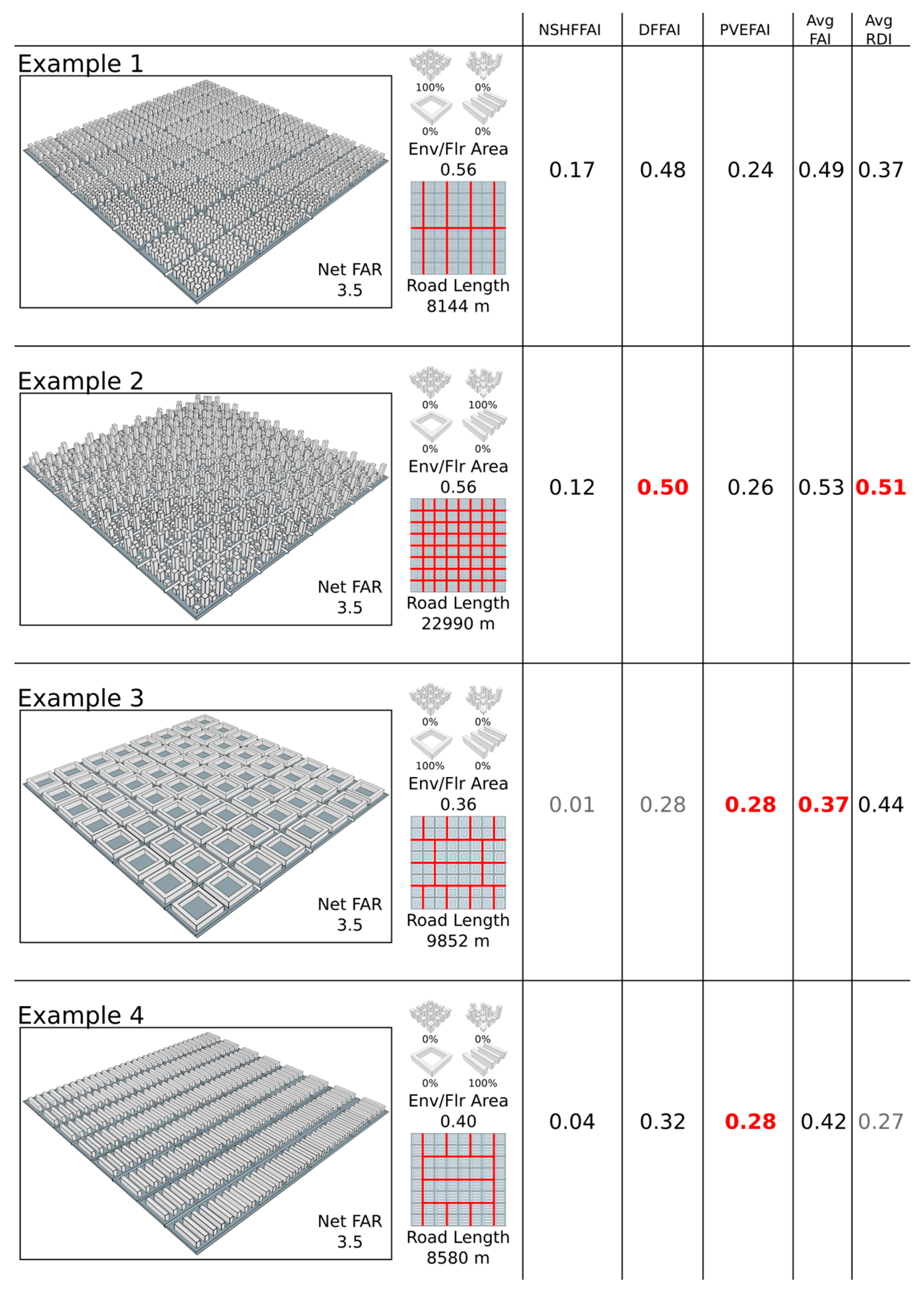
- (1)
- Example 1 consists of tower blocks of uniform heights. The road network has a main spine that connects all the plots.
- (2)
- Example 2 consists of tower blocks of varying heights. The road network is a full grid. For examples 3–6, the road network is a variation of the grid network with a reduced road length.
- (3)
- Example 3 consists of the courtyard blocks.
- (4)
- Example 4 consists of slab blocks.
- (5)
- Example 5 consists of a combination of all four building typologies in equal proportions. The tower blocks of varying heights are in the central area, surrounded by tower blocks of a uniform height. The peripherals are occupied by the courtyard and slab blocks.
- (6)
- Example 6 consists of a combination of all four building typologies in varying proportions. We increased the proportion of tower blocks in the central region of the site.
- (7)
- Example 7 has the same building typologies as example 6. The net FAR is increased by increasing the heights of the blocks. The road network is of a central ring configuration. The configuration is only possible with the increase in land-use plot size (demarcated by a dashed line).
- (8)
- Example 8 is the denser version of examples 6 and 7. The road length of the street network is drastically reduced with the increase in land-use plot size (demarcated by a dashed line).
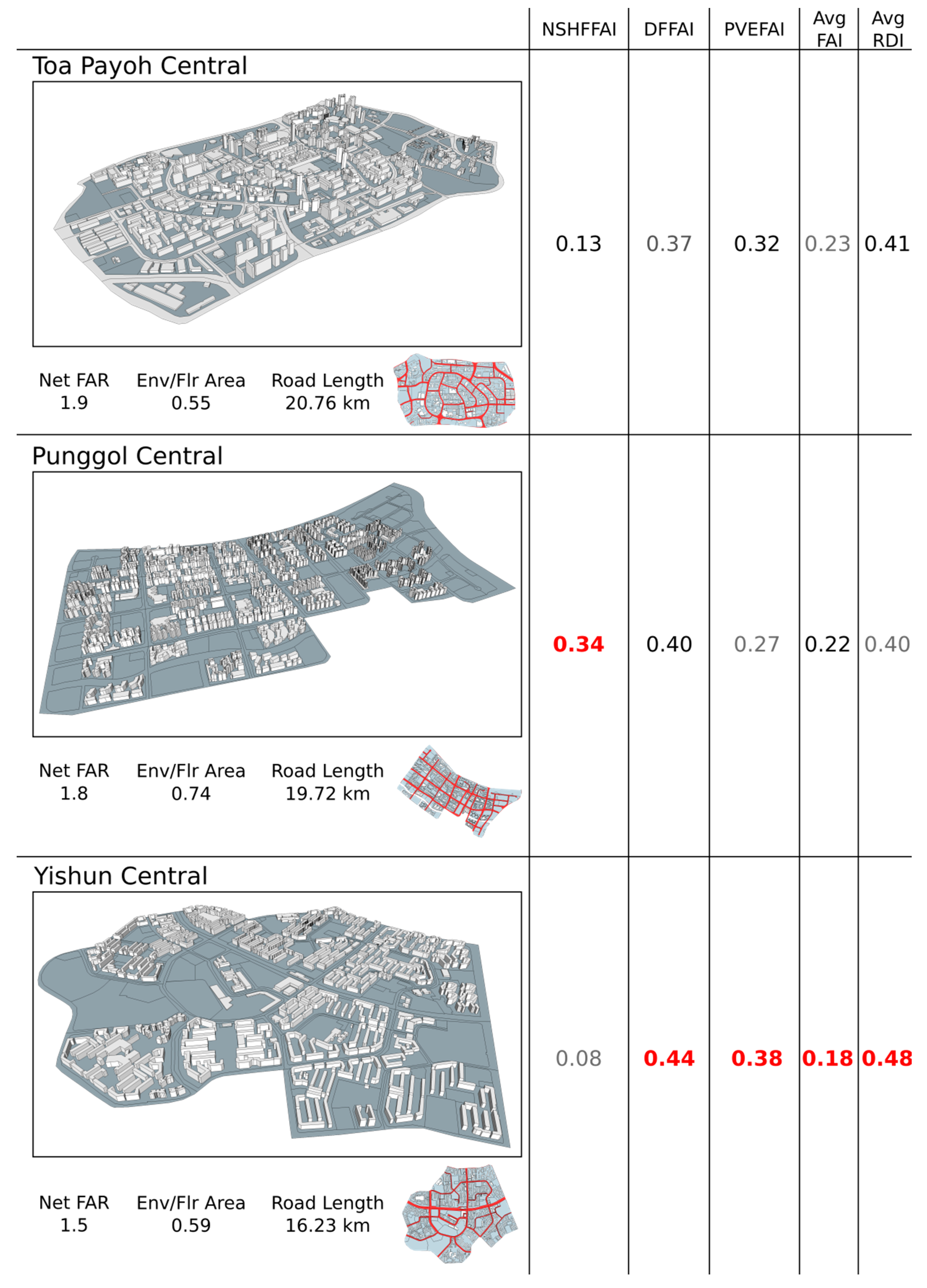
The second case study is more complex than the first case study. It consists of three examples based on existing residential neighbourhood centres in Singapore; Toa Payoh, Yishun, and Punggol (Figure 3 below). The site areas of the examples are 410 ha, 446 ha, and 400 ha, with a varying net FAR of 1.9, 1.5, and 1.8, respectively. This is to show the applicability of the performance indicators in more complex cases resembling real-world scenarios. The three examples were modelled according to the workflow described in our previous study [41].
We calculated the total floor area for each urban area by assuming a floor-to-floor height of 3 m for every building massing. We analysed the FAI for the northeast direction, Singapore’s prevailing wind direction, and the site was divided into a 100m x 100m grid according to Wong and Nichol’s study [34]. The threshold values for the solar analysis are listed in Table 1.
3. Results
The results of the eight examples of case study 1 are shown in Figure 1 and Figure 2, with the best performing results of the eight examples in bold and highlighted in red. The examples showed that the performance indicators are sensitive to all form changes made in the case study. The results of the three examples of case study 2 are shown in Figure 3, with the best performing results in bold and highlighted in red. The examples show that the performance indicators are applicable to more complex cases resembling real scenarios. The results of each case study are described in detail in the next sections. Please refer to the online coloured version of the paper for the false colour figures from Figure 4, Figure 5, Figure 6, Figure 7, Figure 8 and Figure 9.
3.1. Case Study 1
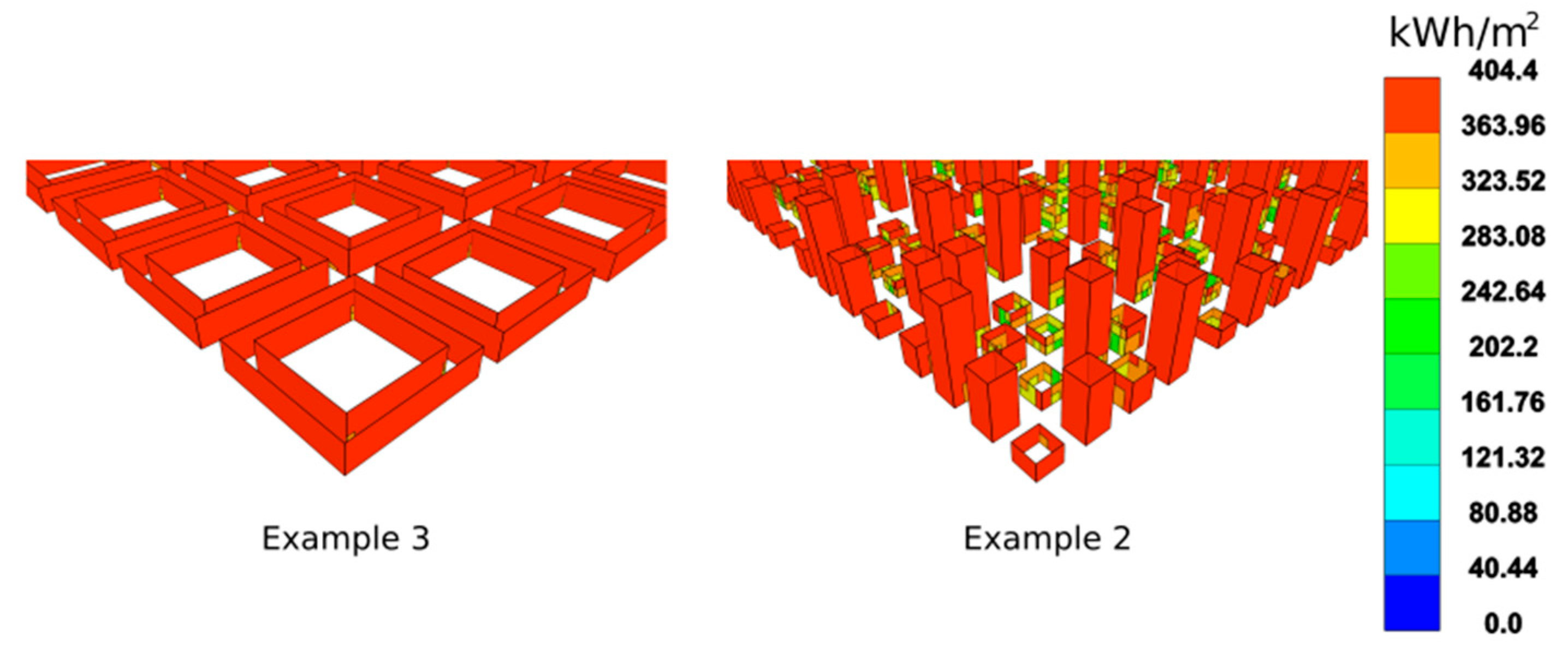
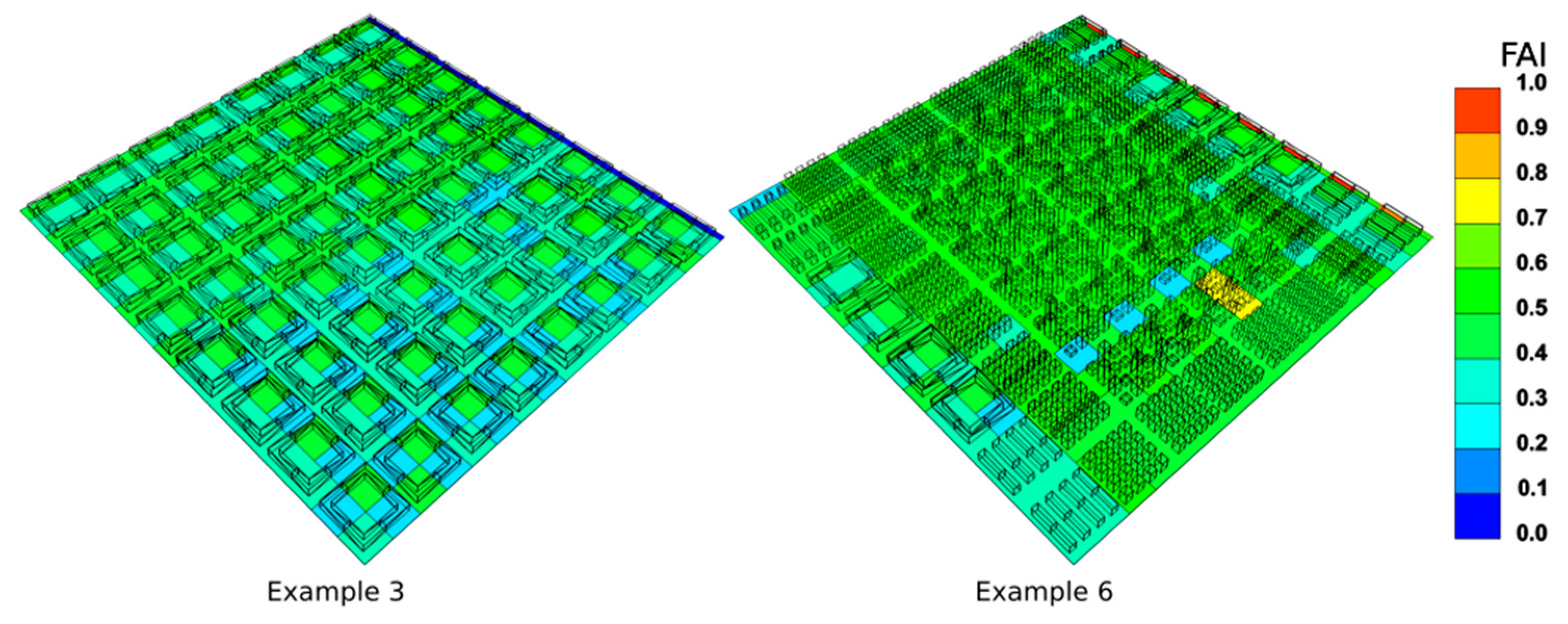
For case study 1, example 3 has the best performing PVEFAI and FAI, while also exhibiting the worst performing NSHFFAI. As shown in Figure 4, the courtyard blocks are fully exposed to solar irradiation compared to example 2, in which the shorter buildings are shaded by the taller buildings. Although examples 3 and 4 are both highly exposed to solar irradiation, they do not have the best performing DFFAI because they have a much lower envelope to floor area ratio. This is the why we used the total floor area as a denominator for measuring solar potential rather than the total façade area. If the total façade area was used as the denominator, examples 3 and 4 would have the best performance in terms of daylight, when that is not the case. Due to its full exposure, example 3 has the best performing PVEFAI. Example 4 has the same PVEFAI due to the same reason. Other than having the best PVEFAI, example 3 also has the lowest FAI due to the large courtyard configuration. This is shown in Figure 5; we can see that the courtyard configuration has a lower wind resistance as compared to the tower blocks in example 6.
From the results, we can see that examples 1 and 2 perform better in terms of NSHFFAI and DFFAI, while examples 3 and 4 perform better in terms of PVEFAI and FAI. The four typologies were mixed in different proportions to obtain balanced performances, which is shown in examples 5 and 6. Example 6 presents the most balanced performances. We then increased the density of example 6 in steps of 0.5 to see how the performance indicators responded. We saw that most results worsen with the increase in density, except NSHFFAI. Example 8 is the densest example and also has the best performing NSHFFAI. This is mainly due to the increase in inter-shading between the buildings as the density increases. Of the deteriorating performance, the FAI increases by the largest degree, showing that the increase in density has the most adverse effect on urban ventilation.
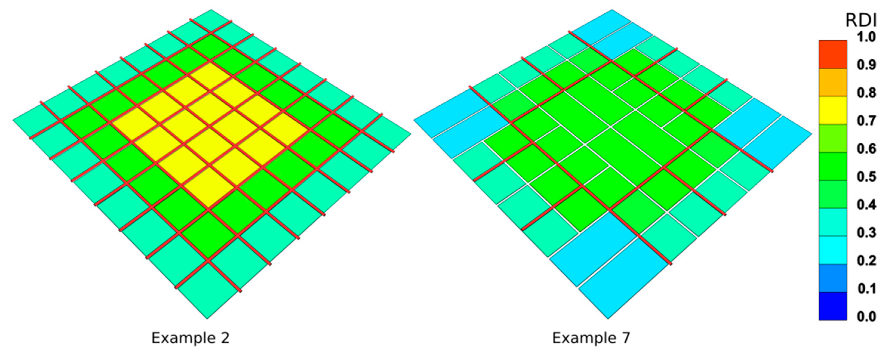
The change in building form has no direct influence on the RDI analysis. Thus, for the case study, we tested a different street network for each example, independent of the building form changes. In real-world scenarios, the building forms on the land-use plots change according to the street network, land-use plot size, and plot shape. Of the different street networks tested, example 2 had a full grid for its street network and the best performing RDI, but at the expense of the longest road length. We tried variations of the grid street network and example 3 was able to achieve a good trade-off between road length and RDI, with 50% fewer roads and a reduction in RDI of only 0.07. Example 7, with a ring road configuration, was able to reduce the road length further by 2448m compared to example 3 by increasing the land-use plot size, while only compromising the RDI by 0.02, as shown in Figure 6.
3.2. Case Study 2
Toa Payoh central is the densest of the three examples in case study 2. Its urban form consists of a mix of tall buildings among short buildings, which increases the PV potential of the tall buildings’ facades as they are unobstructed by the neighbouring shorter buildings. As the buildings are well-spaced, the roof areas of the shorter buildings are able to receive a good amount of solar irradiation. This is in contrast to Punggol central, where the tower blocks are mostly of uniform heights and the PV potential of the building facades is greatly reduced by neighbouring towers. With the appropriate urban form, the denser Toa Payoh central achieves a better PVEFAI than Punggol central, as shown in Figure 7. However, Toa Payoh has the worst DFFAI; most of the PV potential comes from its roof area, and its façade area does not receive as much solar illumination as Punggol, which is shown in Figure 8.
Punggol central has the best performing NSHFFAI, while having the worst performing PVEFAI. This is mainly because of its urban form, where all of the tower blocks are of uniform heights positioned in close proximity to each other. Although it creates inter-shading between towers, it also blocks the daylight and PV potential for each building.
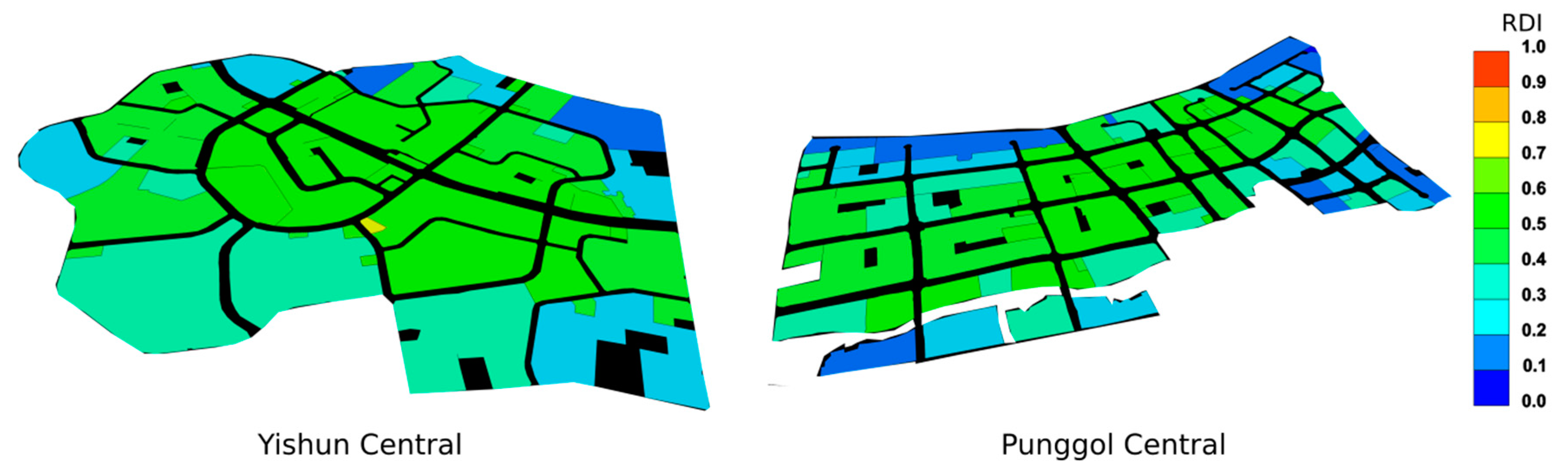
Yishun central has the best performances in DFFAI, PVEFAI, and FAI. Its NSHFFAI is the worst performing of the three examples; the reason for this is that the building forms are fully exposed to solar irradiation, which is similar to the building forms in examples 3 and 4 of the previous case study. It is the least dense of the three examples; the buildings are allowed to be spaced apart to increase daylight, solar, and urban ventilation potentials, as reflected in the DFFAI, PVEFAI, and FAI. Yishun central also has the best-designed street network; with the shortest road length, it is able to achieve the best RDI. The street network is a combination of the main spine with a ring road configuration as shown in Figure 9, which is able to out-perform a grid street network in Punggol.
4. Discussion
We have shown that the performance indicators identified in this research are sensitive to the changes in urban form. The increase in aspect ratio and an increase in density leads to a reduction of PV potential, which is in agreement with the study by Martin et al. [10]. High-rise building forms result in a higher FAI, as shown in the study by Wong et al. [33], compared to the low-rise building forms like the courtyard and slab blocks. A full grid street network has the highest connectivity, as shown in the study by Stangl [39]. In the early design stages with high uncertainty, urban designers are able to use these tendencies as guides to experiment with different urban forms. We have demonstrated this in the first case study, by making improvements to examples 5 and 6. In the second case study, we showed the indicators’ applicability to real-world examples. We were able to sort out the performances of these real-world examples quickly, and their performances can be used as references or precedents for future neighbourhood designs.
There are limitations in using these indicators, which simplify complex phenomena in the built environment, neglect temporal and spatial variation, and provide only a single value at a neighbourhood scale to summarise the condition of the phenomena. Due to the lack of information in the massing design stage, many assumptions were made in calculating the performance indicators. Except for the solar potentials, which are derived from simulation results from a validated backwards ray tracing lighting simulation, Radiance, most of the calculations for these indicators are rudimentary. The indicators are a coarse representation of performance on a neighbourhood scale, which does not provide performance information or ensure a good performance for each individual building.
The solar potentials are solar performances normalised by the total floor area of the neighbourhood. Thus, an urban form with a high solar potential performance can still have poor individual building performances. This is because a few high performing buildings can skew the overall results of the solar potential. This skewing of results can also happen for the connectivity potential, where the RDI is an average of all plots. The disparity in performance for the difference in scale is more complicated for the ventilation potential. The FAI is originally developed as an indicator to map the urban surface roughness on a neighbourhood scale, and it has been shown to correlate with wind speed in an urban context, as mentioned in the studies in Section 2. However, there is a contradiction for ventilation potential between the neighbourhood and building scale. For example, buildings oriented parallel to the prevailing wind direction encourage ventilation on a neighbourhood scale, but the ventilation potential in the building is compromised as the building façades are oriented away from the wind direction [44]. One possible solution to reconcile the differences is to use the FAI to ensure wind flow through the neighbourhood, and to maximise the ventilation potential on a building scale with strategies such as an increase in porosity and the shaping of spaces like sky gardens and atriums [45]. The prediction of wind flow in an urban context is very complicated, and with the limited information, one needs to exercise caution when interpreting the ventilation potential.
Although the demonstration has shown the feasibility of identifying better performing design options with the indicators, as discussed in this section, they are not foolproof, and designers need to have prior urban climate knowledge. These indicators provide a coarse measure of performance that is only useful in a comparative study, where there are multiple design options, and designers want to identify the design options with better performance potentials relative to other design options. The results should not be taken definitively and should not be interpreted independently without a reference or other comparisons. For example, an urban design having a low FAI does not ensure good urban ventilation or inform the designer about wind flow patterns, and a high PVEFAI does not ensure high energy generation from PV.
5. Conclusions
In conclusion, this research has demonstrated the feasibility of using performance indicators to identify urban forms with a high-performance potential in comparative studies. In addition, feedback from visualising the performance results as a false colour diagram enables designers to explore and understand the relationship between urban forms and the performances. Designers can then decide on the urban form with high-performance potential or improve their design according to this feedback.
We envision two future investigations of these performance indicators. First, the indicators can be refined through comparison with either existing energy, daylight, and traffic measurements, or alternatively with validated and detailed simulation results. Examples of refinements include validating and updating the calculations to account for the limitations discussed, updating the solar threshold values, updating the grid size for FAI analysis, and determining the RDI threshold value. Once refined, we can evaluate existing neighbourhoods with the indicators and establish a reference performance benchmark for future urban designs in the tropics. The Python library will facilitate this massive exercise that requires intensive data acquisition and computation power by streamlining the evaluation workflow. Second, these performance indicators can be used as objectives in an optimisation process. The Python library can be readily integrated into an existing optimisation tool for performing optimisation process. Currently, designers are unclear on the performance objectives to optimise in the massing design stage. With an established set of performance indicators, a multi-objective optimisation can be conducted as early as the massing design stage, with the five indicators as performance objectives. The optimisation process can generate very large numbers of design options. We will introduce data exploration techniques for designers to explore these options and understand the trade-offs for their design decisions. For example, through exploring the Pareto front, designers can grasp a good density for achieving a balance between NSHFFAI, DFAI, PVEFAI, and FAI, or the extent of roads and the plot layout for achieving a good RDI.
The performance indicators are implemented in an open Python library, and we welcome any user’s feedback and contribution. Pyliburo is available at [46]. The source codes for evaluating NSHFFAI, DFFAI and PVEFAI are available at [47]. The source codes for evaluating the FAI and RDI are available at [48,49] respectively. Lastly, all the CityGML files for the case studies are available at [50]. We hope that designers will use the performance indicators for choosing massing design with the highest performance potential in the early design stages and be able to utilise these potentials by using detailed performance simulations for design development in the later design stages.
Acknowledgments
This research was supported by the National Research Foundation Singapore through the Singapore MIT Alliance for Research and Technology’s Center for Environmental Sensing and Modeling interdisciplinary research program. This research programme/project is funded by the National Research Foundation (NRF), Prime Minister’s Office, Singapore, under its Campus for Research Excellence and Technological Enterprise (CREATE) programme.
Author Contributions
All authors contributed to this work. Kian Wee Chen conceived and designed the experiment under the guidance of Leslie Norford. Kian Wee Chen performed the experiments and analysed the data. Kian Wee Chen drafted the manuscript, which was revised by Leslie Norford. All authors have read and approved the final manuscript.
Conflicts of Interest
The authors declare no conflict of interest.
Appendix A
The procedure documented in [39] to calculate the RDI is summarised as follows:
- Map the site—define the boundary, route network, obstructions, and plots of the site.
- Designate the peripheral points—place peripheral points on the boundary line based on the intersection of internal routes; the peripheral points are no more than 106.7m (350’) apart from each other.
- Identify plots with high RDI—measure the RDI of each plot to all the peripheral points; if the RDI for any peripheral point is higher than a user-defined RDI value, the plot has poor connectivity. For plots bigger than 2023.4 m2 (0.5 acres), the starting point of the measurement is the centre of the plot; otherwise, the starting point of the measurement is the midpoint of the plot frontage.
- Calculate the score—the score is the fraction of plots with good connectivity, specified by a user-defined RDI value.
Appendix B
The threshold value for NSHFAVI is derived from the ETTV [19], as shown in Equation (A1).
where TDeq is the equivalent temperature difference (K), WWR is the window to wall ratio, ∆T is the temperature difference (K), SF is the solar factor (W/m2), Uw is the thermal transmittance of the opaque wall (W/(m2K)), Uf is the thermal transmittance of the fenestration (W/(m2K)), CF is the solar correction factor for fenestration, and SC is the shading coefficient of fenestration. The ETTV equation considers the three basic components of solar heat gain through the envelope. TDeq(1 − WWR)Uw accounts for the solar heat gain by conduction through opaque walls, ∆T(WWR)Uf accounts for the solar heat gain by conduction through the fenestration, and SF(WWR)(CF)(SC) accounts for the gain by solar radiation through the fenestration.
ETTV = TDeq(1 − WWR)Uw + ∆T(WWR)Uf + SF(WWR)(CF)(SC),
We assumed a worst case scenario of a fully glazed building with a WWR of 1, typical Uf of 2.8 W/(m2K) [51], SC of 0.5, ∆T of 3.4 K, and SF of 211 W/m2 [19]. In order to meet the base ETTV of 50W/m2, as set out in Green Mark [46], the amount of solar irradiation falling on the surface of a building is about 80 W/m2, according to Equation (A2) below.
SF(WWR)(CF) = (ETTV − ∆T(WWR)Uf)/SC
The annual threshold value for NSHFAVI can then be calculated according to Equation (A3) below:
where Threshold Value(NSHFAVI) is the threshold value for NSHFAVI in (kWh/m2), and hdaylight is the annual daylight hours (h). According to the Singapore weather file [52], the annual daylight hours value is 4549 h.
Threshold Value(NSHFAVI) = (SF(WWR)(CF)(hdaylight))/1000,
References
- Jacoby, S. The Urban. In Drawing Architecture and the Urban; John Wiley & Sons, Ltd.: Hoboken, NJ, USA, 2016; pp. 148–241. [Google Scholar]
- Vidmar, J. Parametric Maps for Performance-Based Urban Design: A lateral method for 3D urban design. In Proceedings of the 31st International Conference on Education and Research in Computer Aided Architectural Design in Europe, Delft, The Netherlands, 18–20 September 2013; Faculty of Architecture, Delft University of Technology: Delft, The Netherlands, 2013; Volume 1, pp. 311–316. [Google Scholar]
- Akin, O.; Moustapha, H. Strategic use of representation in architectural massing. Des. Stud. 2004, 25, 31–50. [Google Scholar] [CrossRef]
- Whitford, V.; Ennos, A.R.; Handley, J.F. “City form and natural process”—Indicators for the ecological performance of urban areas and their application to Merseyside, UK. Landsc. Urban Plan. 2001, 57, 91–103. [Google Scholar] [CrossRef]
- Reinhart, C.F.; Dogan, T.; Jakubiec, J.A.; Rakha, T.; Sang, A. UMI—An Urban Simulation Environment for Building Energy Use, Daylighting and Walkability. In Proceedings of the Building Simulation, Chambéry, France, 26–28 August 2013. [Google Scholar]
- Collada Khronos Group. Connecting Software to Silicon. Available online: https://www.khronos.org/collada/ (accessed on 27 October 2016).
- Gröger, G.; Plümer, L. CityGML—Interoperable semantic 3D city models. ISPRS J. Photogramm. Remote Sens. 2012, 71, 12–33. [Google Scholar] [CrossRef]
- Yang, F.; Chen, L. Developing a thermal atlas for climate-responsive urban design based on empirical modeling and urban morphological analysis. Energy Build. 2016, 111, 120–130. [Google Scholar] [CrossRef]
- Oke, T.R. Boundary Layer Climates; University Paperbacks: Methuen, MA, USA, 1987. [Google Scholar]
- De Lemos Martins, T.A.; Adolphe, L.; Bastos, L.E.G.; de Lemos Martins, M.A. Sensitivity analysis of urban morphology factors regarding solar energy potential of buildings in a Brazilian tropical context. Sol. Energy 2016, 137, 11–24. [Google Scholar] [CrossRef]
- Saratsis, E.; Dogan, T.; Reinhart, C.F. Simulation-based daylighting analysis procedure for developing urban zoning rules. Build. Res. Inf. 2016, 45, 1–14. [Google Scholar] [CrossRef]
- Ng, E.; Yuan, C.; Chen, L.; Ren, C.; Fung, J.C.H. Improving the wind environment in high-density cities by understanding urban morphology and surface roughness: A study in Hong Kong. Landsc. Urban Plan. 2011, 101, 59–74. [Google Scholar] [CrossRef]
- Srifuengfung, S. Relationship between Urban Morphological Properties and Ventilation in the Intensely Developed Areas of Inner Bangkok. AU J. Technol. 2012, 16, 63–73. [Google Scholar]
- Curtis, F.A.; Neilsen, L.; Bjornsor, A. Impact of Residential Street Design on Fuel Consumption. J. Urban Plan. Dev. 1984, 110, 1–8. [Google Scholar] [CrossRef]
- Marshall, W.; Garrick, N. Effect of Street Network Design on Walking and Biking. Transp. Res. Rec. J. Transp. Res. Board 2010, 2198, 103–115. [Google Scholar] [CrossRef]
- Portland Metro. Street Connectivity: An Evaluation of Case Studies in the Portland Region; Portland Metro: Portland, OR, USA, 2004. [Google Scholar]
- Frank, L.D.; Stone, B., Jr.; Bachman, W. Linking land use with household vehicle emissions in the central puget sound: Methodological framework and findings. Transp. Res. D Transp. Environ. 2000, 5, 173–196. [Google Scholar] [CrossRef]
- Fong, C.; Wu, X.; Djunaedy, E. Formulating an Alternative Methodology for Singapore’s Envelope Thermal Transfer Value Calculation Accounting for non-conventional shading strategies. In Proceedings of the PLEA2009—26th Conference on Passive and Low Energy Architecture, Quebac City, QC, Canada, 22–24 June 2009. [Google Scholar]
- Chua, K.J.; Chou, S.K. An ETTV-based approach to improving the energy performance of commercial buildings. Energy Build. 2010, 42, 491–499. [Google Scholar] [CrossRef]
- Compagnon, R. Solar and daylight availability in the urban fabric. Energy Build. 2004, 36, 321–328. [Google Scholar] [CrossRef]
- Dogan, T.; Reinhart, C.; Michalatos, P. Urban Daylight Simulation Calculating the Daylit Area of Urban Designs. In Proceedings of the SIMBUILD 2012 Fifth National Conference of IBPSA-USA, Madison, WI, USA, 1–3 August 2012. [Google Scholar]
- Amado, M.; Poggi, F. Towards Solar Urban Planning: A New Step for Better Energy Performance. Energy Procedia 2012, 30, 1261–1273. [Google Scholar] [CrossRef]
- Lobaccaro, G.; Frontini, F.; Masera, G.; Poli, T. SolarPW: A New Solar Design Tool to Exploit Solar Potential in Existing Urban Areas. Energy Procedia 2012, 30, 1173–1183. [Google Scholar] [CrossRef]
- Ward, G.J. The RADIANCE Lighting Simulation and Rendering System. In Proceedings of the SIGGRAPH 94 21st Annual Conference on Computer Graphics and Interactive Techniques, Orlando, FL, USA, 24–29 July 1994. [Google Scholar]
- Robinson, D.; Stone, A. Irradiation modelling made simple: The cumulative sky approach and its applications. In Proceedings of the PLEA2004—The 21st Conference on Passive and Low Energy Architecture, Eindhoven, The Netherlands, 19–21 September 2004. [Google Scholar]
- Golany, G.S. Urban design morphology and thermal performance. Atmos. Environ. 1996, 30, 455–465. [Google Scholar] [CrossRef]
- Emmanuel, R. An Urban Approach to Climate Sensitive Design; Routledge: Abingdon, UK, 2005. [Google Scholar]
- Ramponi, R.; Blocken, B.; de Coo, L.B.; Janssen, W.D. CFD simulation of outdoor ventilation of generic urban configurations with different urban densities and equal and unequal street widths. Build. Environ. 2015, 92, 152–166. [Google Scholar] [CrossRef]
- Ahmad, K.; Khare, M.; Chaudhry, K.K. Wind tunnel simulation studies on dispersion at urban street canyons and intersections—a review. J. Wind Eng. Ind. Aerodyn. 2005, 93, 697–717. [Google Scholar] [CrossRef]
- Burian, S.J.; Brown, M.J.; Linger, S.P. Morphological Analyses Using 3D Building Databases: Los Angeles, California; Los Alamos National Laboratory: Los Alamos, NM, USA, 2002. [Google Scholar]
- Burian, S.J.; Velugubantla, S.P.; Brown, M.J. Morphological Analyses Using 3D Building Databases: Phoenix, Arizona; Los Alamos National Laboratory: Los Alamos, NM, USA, 2002. [Google Scholar]
- Grimmond, C.S.B.; Oke, T.R. Aerodynamic Properties of Urban Areas Derived from Analysis of Surface Form. J. Appl. Meteorol. 1999, 38, 1262–1292. [Google Scholar] [CrossRef]
- Wong, M.S.; Nochol, J.E.; Ng, E.Y.Y.; Guilbert, E.; Kwok, K.H.; To, P.H.; Wang, J.Z. GIS Techniques for Mapping Urban Ventilation, Using Frontal Area Index and Least Cost Path Analysis. Int. Arch. Photogramm. Remote Sens. Spat. Inf. Sci. 2010, 38, 586–591. [Google Scholar]
- Wong, M.S.; Nichol, J.E. Spatial variability of frontal area index and its relationship with urban heat island intensity. Int. J. Remote Sens. 2013, 34, 885–896. [Google Scholar] [CrossRef]
- Dill, J. Measuring network connectivity for bicycling and walking. In Proceedings of the 83rd Annual Meeting of the Transportation Research Board, Washington, DC, USA, 11–15 January 2004; pp. 11–15. [Google Scholar]
- Knight, P.L.; Marshall, W.E. The metrics of street network connectivity: Their inconsistencies. J. Urban. Int. Res. Placemaking Urban Sustain. 2015, 8, 241–259. [Google Scholar] [CrossRef]
- Ozbil, A.; Peponis, J.; Stone, B. Understanding the link between street connectivity, land use and pedestrian flows. Urban Des. Int. 2011, 16, 125–141. [Google Scholar] [CrossRef]
- Stangl, P.; Guinn, M.J. Neighborhood design, connectivity assessment and obstruction. Urban Des. Int. 2011, 16, 285–296. [Google Scholar] [CrossRef]
- Stangl, P. The pedestrian route directness test: A new level-of-service model. Urban Des. Int. 2012, 17, 228–238. [Google Scholar] [CrossRef]
- Chen, K.W.; Janssen, P.; Norford, L. Automatic Generation of Semantic 3D City Models from Conceptual Massing Models. In Proceedings of the CAAD Futures 2017, Istanbul, Turkey, 12–14 July 2017. [Google Scholar]
- Chen, K.W.; Norford, L.K. Workflow for Generating 3D Urban Models from Open City Data for Performance-Based Urban Design. In Proceedings of the Asim 2016 IBPSA Asia Conference, Jeju, Korea, 27–29 November 2016. [Google Scholar]
- Martins, T.A.L.; Adolphe, L.; Bastos, L.E.G. From solar constraints to urban design opportunities: Optimization of built form typologies in a Brazilian tropical city. Energy Build. 2014, 76, 43–56. [Google Scholar] [CrossRef]
- Luther, J.; Reindl, T. Solar Photovoltaic (PV) Roadmap for Singapore (A Summary); Solar Energy Research Institute of Singapore (SERIS): Singapore, 2013. [Google Scholar]
- Givoni, B. Urban design for hot humid regions. Renew. Energy 1994, 5, 1047–1053. [Google Scholar] [CrossRef]
- Building and Construction Authority (BCA). Building Planning and Massing; Green Building Platinum Series; The Centre for Sustainable Buildings and Construction; Building and Construction Authority: Singapore, 2010. [Google Scholar]
- Chen, K.W. Pyliburo. Available online: https://github.com/chenkianwee/pyliburo (accessed on 7 June 2017).
- Chen, K.W. Pyliburo Example Files. Available online: https://github.com/chenkianwee/pyliburo_example_files/blob/master/example_scripts/citygml/analyse_citygml_solarsim.py (accessed on 7 June 2017).
- Chen, K.W. Pyliburo Example Files. Available online: https://github.com/chenkianwee/pyliburo_example_files/blob/master/example_scripts/citygml/analyse_citygml_fai.py (accessed on 7 June 2017).
- Chen, K.W. Pyliburo Example Files. Available online: https://github.com/chenkianwee/pyliburo_example_files/blob/master/example_scripts/citygml/analyse_citygml_rdi.py (accessed on 7 June 2017).
- Chen, K.W. Pyliburo Example Files. Available online: https://github.com/chenkianwee/pyliburo_example_files/tree/master/example_files/mdpi_urbform_eg/citygml (accessed on 7 June 2017).
- BCA Singapore. BCA Green Mark for New Non-Residential Buildings Version NRB/4.1; BCA: Singapore, 2013. [Google Scholar]
- EnergyPlus. Weather Data by Region. Available online: https://energyplus.net/weather-region/southwest_pacific_wmo_region_5 (accessed on 6 February 2017).
Figure 1.
Comparison of the first four variations of the first case study (examples 1–4). The best performance indicators are highlighted in red and bold.
Figure 1.
Comparison of the first four variations of the first case study (examples 1–4). The best performance indicators are highlighted in red and bold.

Figure 2.
Comparison of the last four variations of the first case study (examples 5–8). The best performance indicators are highlighted in red and bold.
Figure 2.
Comparison of the last four variations of the first case study (examples 5–8). The best performance indicators are highlighted in red and bold.
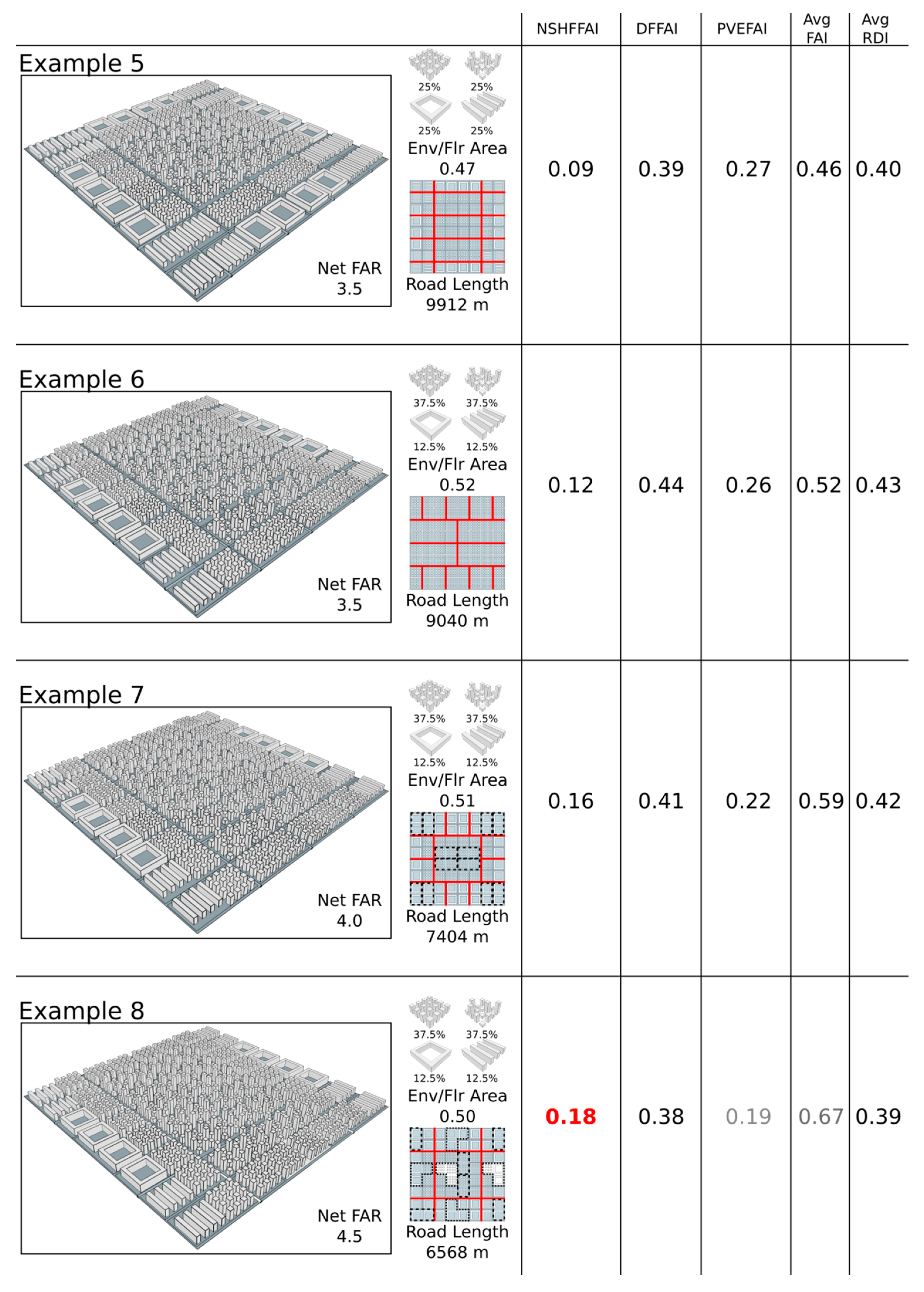
Figure 3.
Comparison of three examples based on neighbourhood centres in Singapore. The best performance indicators are highlighted in red and bold.
Figure 3.
Comparison of three examples based on neighbourhood centres in Singapore. The best performance indicators are highlighted in red and bold.

Figure 4.
Courtyard blocks are fully exposed to solar irradiation as compared to the tower blocks.

Figure 5.
Courtyard blocks have less wind resistance than tower blocks.

Figure 6.
Example 7 is able to reduce the road length while achieving a similar RDI performance by enlarging the plot size.
Figure 6.
Example 7 is able to reduce the road length while achieving a similar RDI performance by enlarging the plot size.

Figure 7.
The varying tower block height in Toa Payoh enables a better performing PVEAVI compared to the uniform block height in Punggol.
Figure 7.
The varying tower block height in Toa Payoh enables a better performing PVEAVI compared to the uniform block height in Punggol.
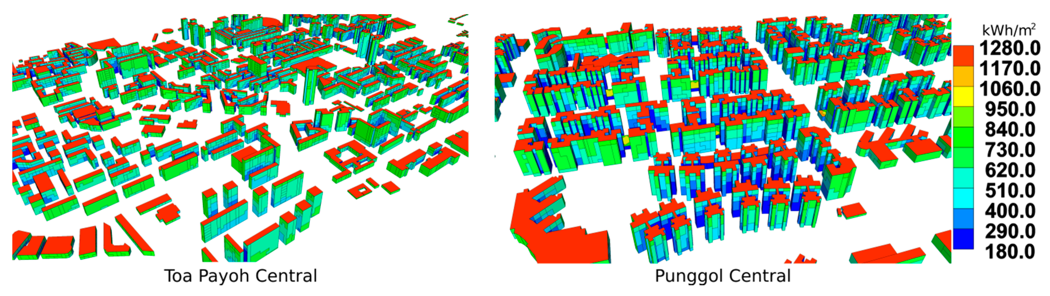
Figure 8.
Toa Payoh central DFFAI performance in comparison to Punggol. The shorter buildings in Toa Payoh have a poorer performance due to the smaller façade area.
Figure 8.
Toa Payoh central DFFAI performance in comparison to Punggol. The shorter buildings in Toa Payoh have a poorer performance due to the smaller façade area.
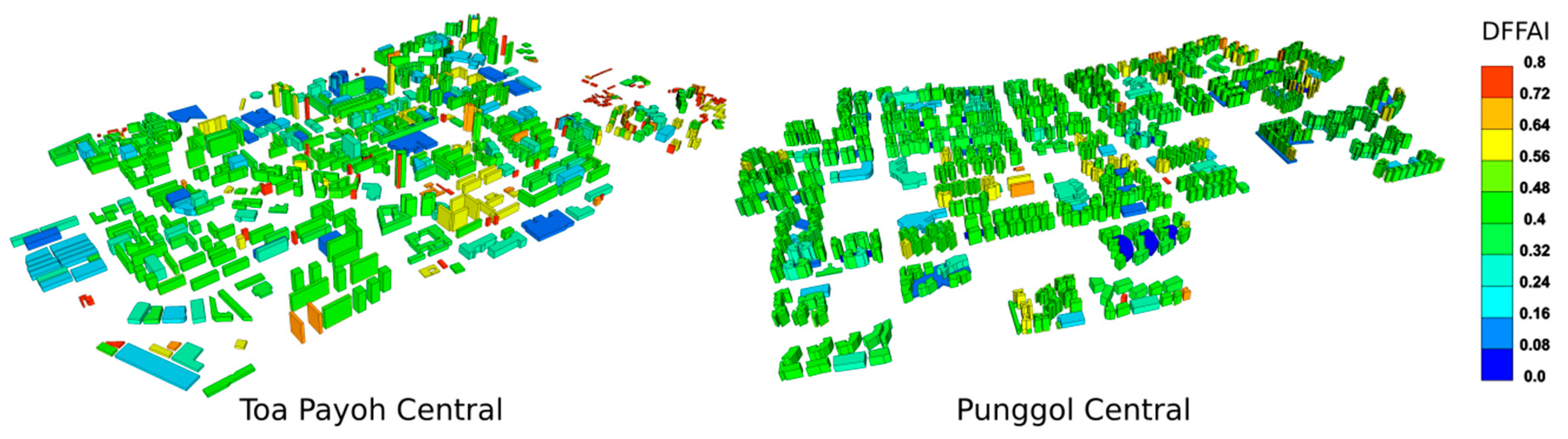
Figure 9.
Yishun central with a spine and ring road configuration is able to out-perform the connectivity of the grid street network in Punggol.
Figure 9.
Yishun central with a spine and ring road configuration is able to out-perform the connectivity of the grid street network in Punggol.


Table 1.
Threshold values for solar potential.
| Solar Performance Indicator | Threshold Value |
|---|---|
| NSHFFAI | 364 kWh/m2 (Details in Appendix B) |
| DFFAI | 10,000 lx [42] |
| PVEFAI | 1280 kWh/m2 [43] |
| PVEFAI | 512 kWh/m2 [43] |
© 2017 by the authors. Licensee MDPI, Basel, Switzerland. This article is an open access article distributed under the terms and conditions of the Creative Commons Attribution (CC BY) license (http://creativecommons.org/licenses/by/4.0/).
Share and Cite
MDPI and ACS Style
Chen, K.W.; Norford, L. Evaluating Urban Forms for Comparison Studies in the Massing Design Stage. Sustainability 2017, 9, 987. https://doi.org/10.3390/su9060987
AMA Style
Chen KW, Norford L. Evaluating Urban Forms for Comparison Studies in the Massing Design Stage. Sustainability. 2017; 9(6):987. https://doi.org/10.3390/su9060987
Chicago/Turabian StyleChen, Kian Wee, and Leslie Norford. 2017. "Evaluating Urban Forms for Comparison Studies in the Massing Design Stage" Sustainability 9, no. 6: 987. https://doi.org/10.3390/su9060987
Note that from the first issue of 2016, this journal uses article numbers instead of page numbers. See further details here.