
Comparison between Inverse Model and Chaos Time Series Inverse Model for Long-Term Prediction

Division of Architecture, Architectural Engineering and Civil Engineering, Sunmoon University, Asan, Chungnam 336-708, Korea
Sustainability 2017, 9(6), 982; https://doi.org/10.3390/su9060982
Submission received: 20 April 2017
/
Revised: 22 May 2017
/
Accepted: 6 June 2017
/
Published: 7 June 2017
(This article belongs to the Section Sustainable Engineering and Science)
Abstract
:This paper presents an inverse model using chaotic behaviour. The chaos time series inverse model, which uses coupling methods between an inverse model and chaos theory can reconstruct a deterministic and low-dimensional phase space by transforming irregular behaviours of nonlinear time-varying systems into a strange attractor (e.g., a Rossler attractor or a Lorenz attractor), and it can then predict future states. For this study, the author used a training dataset measured in an existing high-rise building and examined the predictive abilities of the chaos time series inverse model modelled into phase spaces with strange attractors in comparison with those of the Support Vector Regression (SVR) out of the inverse model. The paper discusses the effective use of the chaos time series inverse model for multi-step ahead prediction.
1. Introduction
Recently, the Building Energy Management System (BEMS) has been used to operate various building systems (dynamic blinds, lights, boiler, chiller, fan, pump, etc.). Model Predictive Control (MPC), which has been used for robust BEMS, is based on sensor data, a mathematical model of the systems, and optimization techniques. In general, optimal control logic in the MPC is an iterative process to search for optimal control variables that minimize a cost function over a time horizon for a given system. The time horizon usually consists of multiple sampling times. Afram and Janabi-Sharifi [1] showed that MPC for Heating, Ventilation and Air Conditioning (HVAC) system control has the advantages of providing better performance and transient response than other control methods (on/off control, Proportional (P)/Proportional Integral (PI)/Proportional Integral Derivate (PID) control, etc.). They indicated that system models, disturbance predictions such as climate data, time horizon, and optimization techniques for accuracy, and reliable MPC runs are major considerations. In particular, the system model, which can be divided into a forward model and an inverse model [2], must be carefully chosen.
The forward model can predict the system’s behaviours using Building Performance Simulation (BPS) tools (e.g., EnergyPlus, ESP-r, and TRNSYS), which are based on first-principles (heat transfer and thermodynamics). Such BPS tools have been used for real-time MPC by coupling with middleware programs (MLE+ [3], BCVTB [4], and FMU [5], etc.). However, it is not easy to develop a robust first principles-based simulation model due to many unknown inputs. In particular, the unknown inputs inherited in the model cause model uncertainties. Calibration processes can be used to remedy this. Heo [6] showed that a stochastic calibration technique (i.e., Bayesian calibration) in an optimization routine could sufficiently improve performance qualities. However, it should be noted that the models coupled with the calibration technique may not be suitable in terms of real-time MPC runs, since the BPS tools integrated with the calibration techniques require extensive computation time.
In contrast, the inverse model has been accepted as a surrogate for the first-principle model due to the recent development of machine learning techniques. The inverse model is constructed based on observed data and machine learning algorithms. If measured data are available and reliable, it demands less computation time and modelling effort compared to the conventional BPS tools. In general, examples of the inverse model include the Auto Regressive Integrated Moving Average (ARIMA), Artificial Neural Network (ANN), Support Vector Regression (SVR), and Gaussian Process Model (GPM). Most previous studies have showed that the aforementioned inverse models are able to produce relatively accurate outputs, and can be used for reliable MPC runs. Niu et al. [7] presented a data-driven SVR with a data mining technology for forecasting short-term electric power load, and insisted that SVR is effective in power load forecasting. Kim and Park [8] showed real-time stochastic MPC formulations and processes of a chiller system using a coupling between Genetic Algorithm (GA) and GPM. They found that a stochastic GPM based on the correlation between observed data can account for model uncertainty, and can find reliable optimal control variables (outlet temperatures of chilled water loop and cooling tower loop) in feasible regions. Kiguchi et al. [9] suggested a GPM for predicting Photovoltaic (PV) generation and on-site consumption, and showed that the developed GPM in terms of an excess-generation model could produce much higher prediction performance than the decoupled value. However, it should be noted that their robustness significantly depends on the qualities of the observed data. When a system is influenced by complex and dynamic interactions with other HVAC systems and when dominant time-varying data are not measured (or are not available during the development of the model), the inverse models usually fail to produce a performance prediction. For example, occupants’ behaviour is a dominant unknown input influencing the output prediction, and is usually hard to reflect in the inverse models. Hence, the inverse models usually produce probabilistic outputs with high variances.
For reliable performance prediction of the inverse model, this study presents a chaos time series inverse model using a coupling method between SVR and chaos theory. The chaos time series inverse model can reconstruct a deterministic and low-dimensional phase space by transforming irregular behaviours of nonlinear time-varying systems into a strange attractor (e.g., a Rossler attractor or a Lorenz attractor), and can then predict future states. Karatasou and Santamouris [10] and Wang et al. [11] showed that a chaos time series inverse model based on phase space dynamics can provide accuracy and reliable performance predictions. Previous chaos studies presented remarkable results for forecasting the behaviours of systems. However, questions remain about multi-step ahead prediction.
With the aforementioned concepts in mind, this study aims to compare the inverse model (SVR) with the chaos time series inverse model (Chaos SVR) in terms of multi-step ahead prediction. The SVR has been widely used for the prediction of building systems. In particular, the SVR has excellent prediction capabilities compared with other inverse models [12]. For this study, total electric energy consumption acquired in an existing office building was chosen as the training data. The comparison was made by focusing on the multi-step ahead prediction. The prediction abilities of the models were assessed in terms of the Mean Bias Error (MBE) and Coefficient of Variance of the Root Mean Square Error (CVRMSE), as suggested by [13].
2. Chaos Time Series Inverse Model
The physical phenomena of real building systems are complex and transient, where a variation of the initial state of a certain system may influence overall systems. In other words, variation of the initial state of a system may cause a critical state or tipping-point of an interconnected system, and then have a significant effect on its performance. For example, occupants’ behaviours affect control of openings (windows or doors) and systems (blinds, lights, HVAC systems, etc.). Occupants move between rooms or respond to system information or environment such as indoor temperature. Such actions influence various building systems’ functions as well as performance indicators (e.g., energy consumption, indoor air quality). To deal with issues of occupants’ behaviours, various stochastic models (e.g., Humphreys algorithm [14], Hidden Markov Chain model [15], and probit model [16]) were developed and validated. However, Andersen et al. [17] insisted that “most validation processes do not go beyond assessing the performance predictions on the very same dataset the model was inferred from” (p. 106). They found that the validation results may lead to significant performance gaps between measured data and predicted outputs if previous stochastic occupant behaviour models were tested using external or other datasets. This means that stochastic behaviour models are suitable when occupants’ behaviours in a given target building are measured. However, in the real BEMS installed in various sensor devices, it is not easy to acquire the data for occupants’ behaviours due to privacy protection, high installation and maintenance costs of sensor devices, etc.
In these conditions, building systems are influenced by such occupants’ behaviours, and can result in an unexpected state or tipping-point according to variations in their initial states. Since, an individual action can have an important bearing on other occupants’ cognitive thinking, as well as on the physical states of building systems. In other words, it can be inferred that real systems are very sensitive to small changes (e.g., the control of openings). This sensitivity of the initial states is called the ‘butterfly effect’. However, most inverse models (e.g., ARIMA, ANN, SVR, and GPM) are not able to reflect the aforementioned unexpected phenomena incurred from the butterfly effect, and may provide predictions with high variances due to unmeasured dominant inputs (e.g., occupants’ behaviours). Otherwise, the aforementioned phenomena can be modelled as a chaos state in random time series data.
The chaos behaviours in time series data can be identified using a Lyapunov exponent [18] and a Hurst exponent [19]. The Lyapunov exponent is a method to quantify the sensitivity of the initial states, termed the butterfly effect, whereby great changes are generated from the small changes in a given condition. If the Lyapunov exponent is positive, the time series data include chaos behaviours having an exponential divergence of the trajectories. Otherwise, the negative Lyapunov exponents are characteristic of non-conservative systems. The Hurst exponent, which has a value in the range from 0.0 to 1.0, can be used to pick out a fractal geometry from time series data. If the Hurst exponent indicates between 0.5 and 1.0, the time series data include the chaos behaviours. Otherwise, it means a random walk against the chaos behaviours. The random walk is a mathematical formalization of a path that consists of a succession of random steps [20]. In other words, the Lyapunov exponent and Hurst exponent can be used to find manifestation of chaos behaviours in the given time series data.
Chaos theory reconstructs the complex irregular behaviours of nonlinear systems into a phase space with deterministic rules such as a strange attractor [10,11], if the time series data prove to be in a chaos state according to aforementioned methods (Lyapunov exponent and Hurst exponent). The chaos time series inverse model can be developed by coupling between the reconstructed phase space and the inverse model. According to Taken’s theory [21], one-dimensional time series data x(t) can be transformed into a state vector z(t) by calculating an embedding dimension d and time delay , as shown in Equation (1). The embedding dimension and time delay are calculated using a False Nearest Neighbour (FNN) algorithm and an Average Mutual Information (AMI), respectively. The reconstructed d-dimensional phase space can be used to predict the next time horizon throughout the inverse model F(zt), as shown in Equation (2).
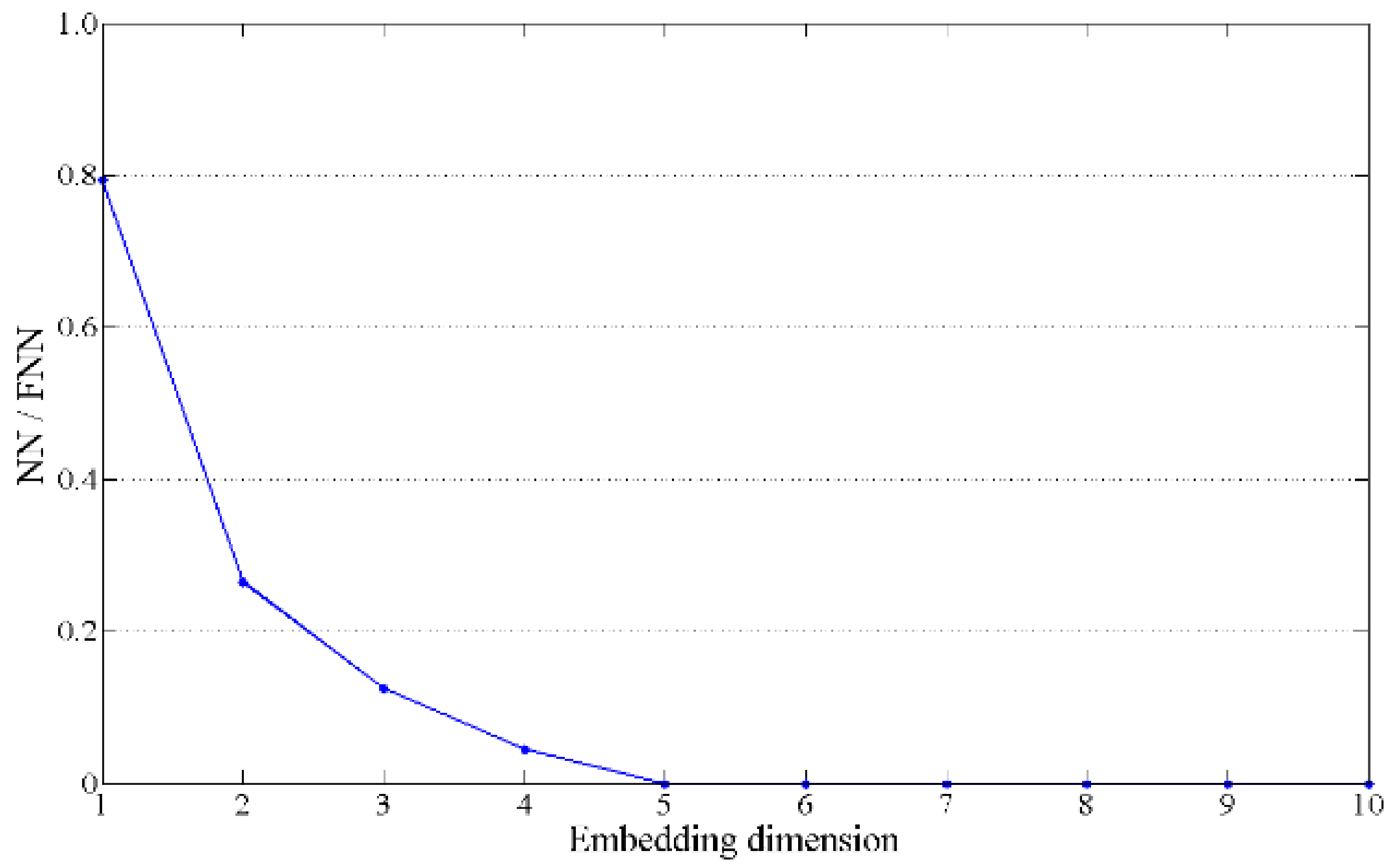
The FNN algorithm proposed by [22] is used to estimate the minimal sufficient embedding dimension. When state vectors are reconstructed while a random embedding dimension is increased, the state vectors are divided into their nearest neighbours ( in Equation (3)) and false nearest neighbours ( in Equation (4)) according to the Euclidean distance of each state vector. The closer to the embedding dimension FNN ratio ( in Equation (5)) gets, the less the FNN ratio becomes. Based on the aforementioned characteristics, the embedding dimension can be obtained using the FNN ratio.
The AMI developed by [23] is used to calculate the time delay of nonlinear data. It can quantify the dependency between the pairs of random variables through the entropy of their joint probability density function, as shown in Equation (6). The AMI determines the delay time for the phase space from the first minimum time.
In this study, the one-dimensional time series data identified as a chaos state using the Lyapunov exponent and Hurst exponent are reconstructed as a d-dimensional phase space using the aforementioned FNN algorithm and AMI. The phase space is used to predict outputs of the next time horizon through a coupling with the inverse model.
3. Support Vector Regression (SVR)
To construct the inverse model and the chaos time series inverse model, SVR was chosen. As mentioned in previous studies [7,24,25,26], SVR can be formulated to a linear regression f(x) with a weight factor , a high-dimensional feature space , and a threshold value b, as shown in Equations (7) and (9). is expressed as non-negative Lagrange multipliers , training input samples xi, and target values yi. denotes a set of nonlinear transformations for mapping the training input samples xi with target values yi. The linear regression was reformulated using the Lagrange multipliers and kernel matrix , as shown in Equations (10) and (11).
To estimate the weight factor and threshold value b, the linear regression model is required. The linear regression model results in a quadratic programming optimization problem. In this study, the optimization problem is constrained by a set of inequality equations with canonical hyperplanes, as shown in Equations (12) and (13). denotes a penalty parameter which is a constant to determine the trade-off between training error and model flatness [26]. denotes a slack variable used to deal with noise errors in the data. With the Lagrange multipliers , the optimization problem can be expressed as shown in Equation (14). To maximize the Lagrange multipliers in the cost function, Equations (14)–(16) are obtained. It should be noted that the predictability of the SVR was influenced by estimates of three unknown parameters (, , and ). To estimate such parameters, various optimization techniques (e.g., gradient based optimization, Genetic Algorithm (GA), Particle Swarm Optimization (PSO)) can be used. In the study, the gradient based optimization was used. It has the advantage of finding an optimal solution quickly in the feasible region.
4. SVR vs. Chaos Time Series Inverse Model
4.1. Target Building and Training Data
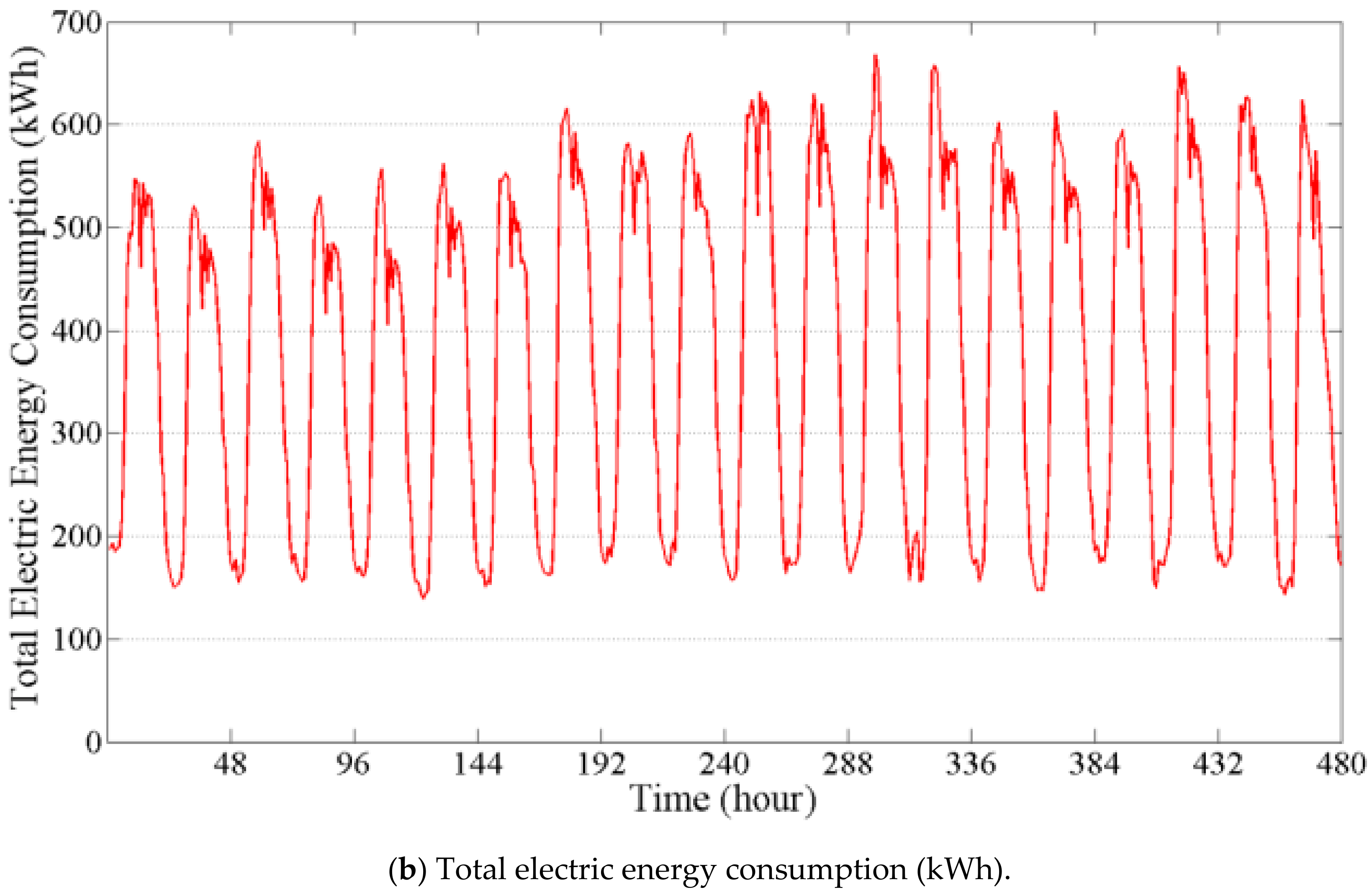
An existing high-rise office building was selected. The building has 10 stories above ground and three underground levels. In this study, the BEMS data were used including total electric energy consumption at a sampling time of 1 h during 20 weekdays in July (Figure 1). The BEMS data were used as training and validating data for constructing two inverse models (SVR and chaos time series inverse model) based on machine learning and chaos theory. The data were divided as follows: (1) 15 days for development of the model, (2) 5 days for validation of the model.
4.2. Comparison between SVR and Chaos Time Series Inverse Model
Figure 2 only shows an architecture of inverses models for formulating a SVR and Chaos time series inverse model in terms of 1-step ahead prediction. A training dataset D of n observations consist of training input data and training output data reflecting different time delays according to k-steps. With the training dataset, the inverse models were constructed using a linear regression model. When the new inputs were given, it was able to predict outputs of next time horizon. If the k-step (2, 3, 4, 5, and 6) was increased, training input and output data were set to and , respectively. In the example, training input and output data for two-step ahead prediction were set to and , respectively, and then it was possible to obtain the predicted outputs using the new data inputs .
Before attempting development of the chaos time series inverse model, the Lyapunov exponent and Hurst exponent were calculated to identify whether or not the time series data were in the chaos state. The Lyapunov exponent and Hurst exponent results were 1.62 and 0.56, respectively. Since the Lyapunov exponent is positive, and the Hurst exponent is more than 0.5, the obtained time series data include characteristics of chaotic behaviour. Based on the chaos state in the given data, the embedding dimension and time delay were calculated using the FNN algorithm and AMI to reconstruct the d-dimensional phase space with state vectors in the chaos time series inverse model.
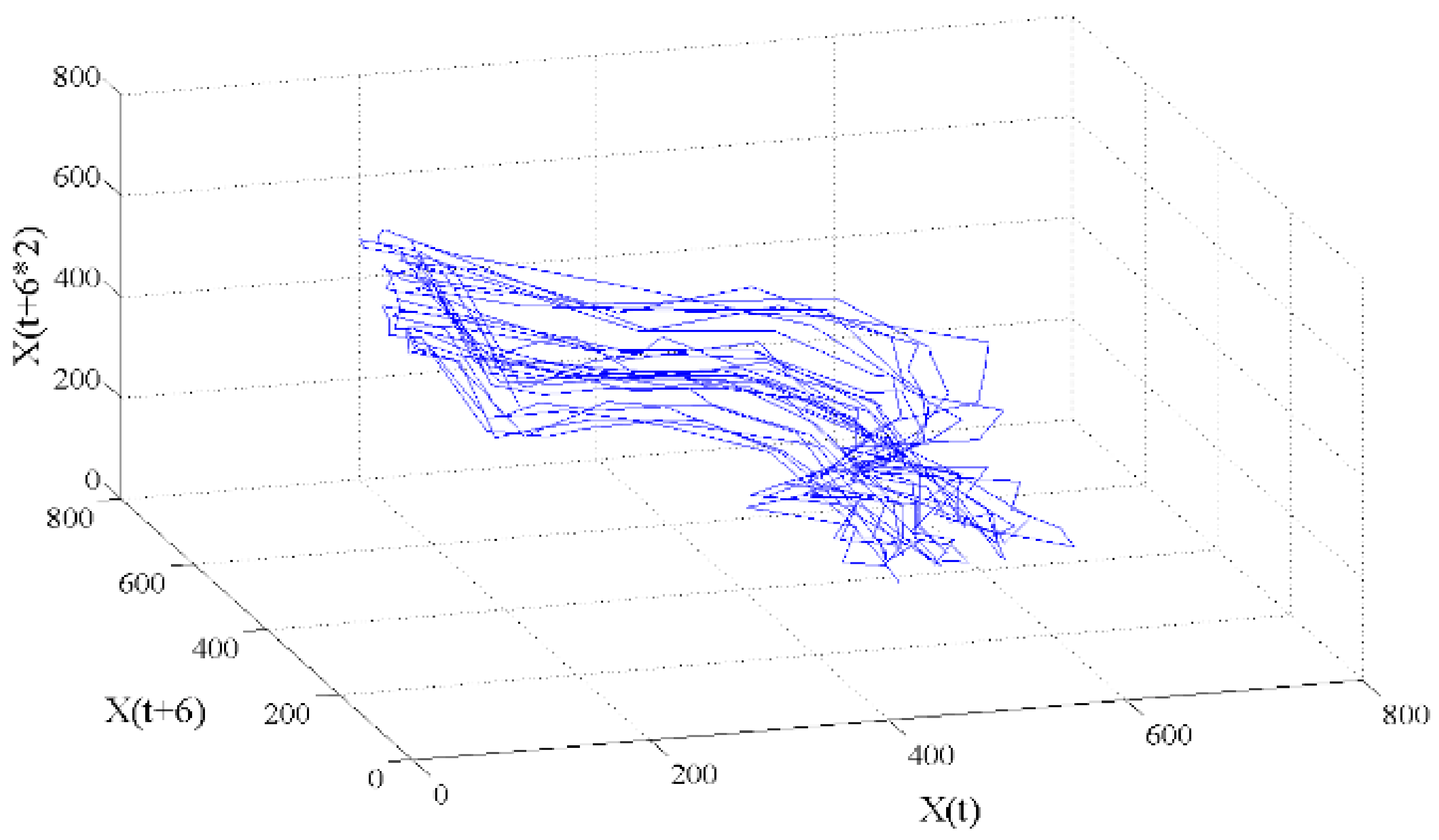
Figure 3 and Figure 4 show the results of the embedding dimension and time delay calculated by the FNN algorithm and AMI, respectively. The calculated embedding dimension and time delay were 5 and 6, respectively. Figure 5 shows the 3D projection (i.e., ‘strange attractor’) of 5D phase space having a delay time of 6 h, resulting from the measured one-dimensional time series data. The strange attractor suggested by [27], which can be represented geometrically in d-dimensional phase space, formulates repeating patterns in the d-dimensional phase space having the delay time, and the orbit or trajectory of the strange attractor moves in a deterministic but unpredictable manner [28]. Due to the deterministic manner, it can capture dynamic natures of nonlinear systems using the flow of a curve with the observed finite set of points, and such repeating patterns can be used to predict future states. In other words, the measured raw BEMS data, which were dependent on the embedding dimension and time delay, were transformed into new vector time series (1D → 5D phase space having a delay time of 6). The new vector times series were used as training data for the inverse model. In other words, the chaos time series inverse model is constructed by coupling between new vector time series and inverse model (SVR). Due to an increase of dimensionality, the chaos time series model (Chaos SVR) has a minor increase in computation cost in comparison to the inverse model (SVR). However, the difference in computation speed between Chaos SVR and SVR is imperceptible.
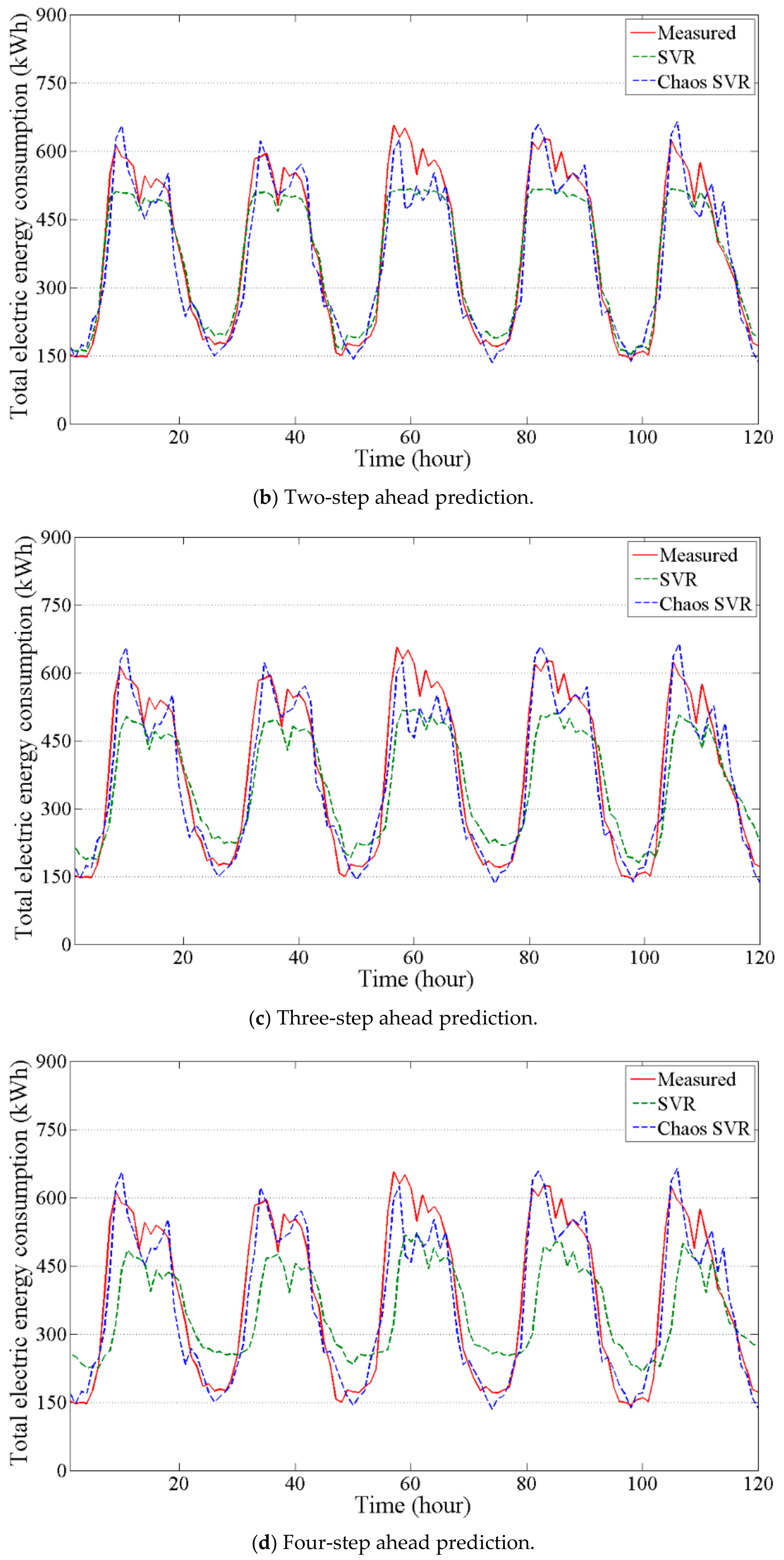
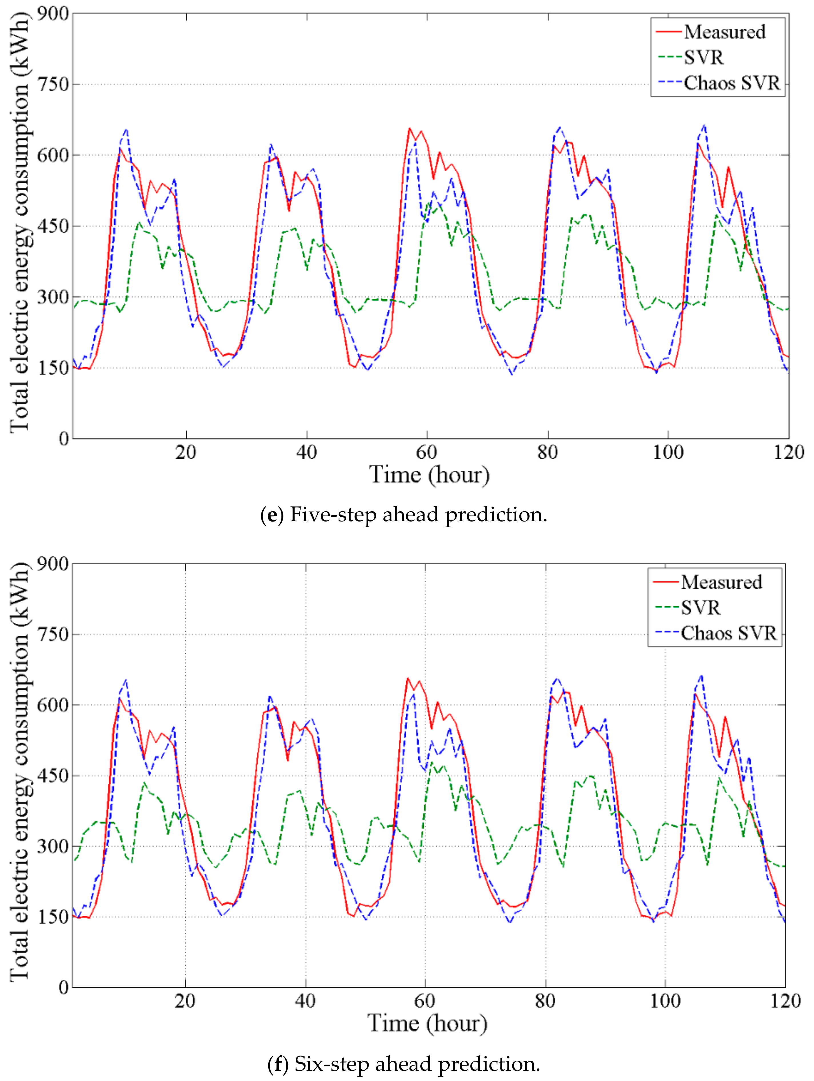
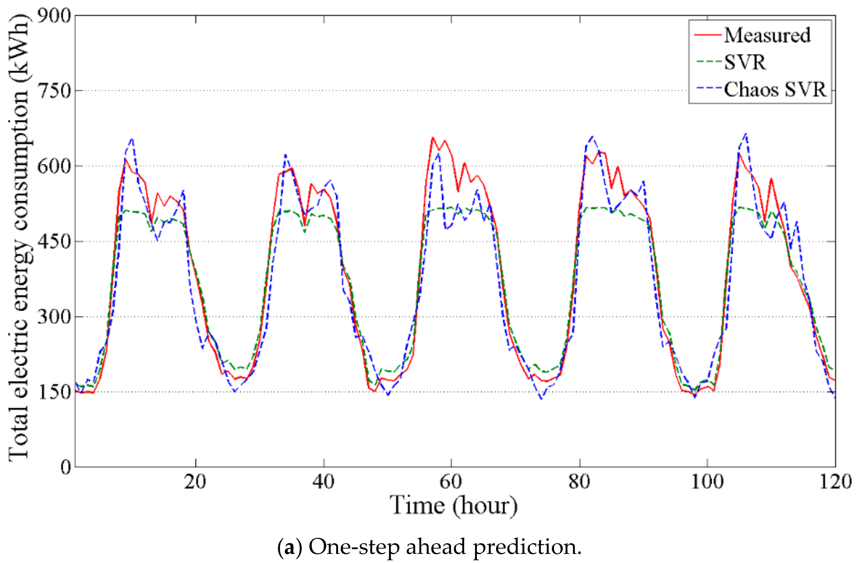
Figure 6 shows the predicted outputs of the inverse model (SVR) and chaos time series inverse model (Chaos SVR) with varying k-steps (1, 2, 3, 4, 5, and 6). When the number of steps (k) increased, the prediction accuracy of the SVR significantly decreased. It can be inferred that the SVR was unsuitable for multi-step ahead predictions (e.g., for multi-step ahead MPC). On the other hand, the prediction accuracy of the Chaos SVR using state orbits of the reconstructed d-dimensional phase space was good compared to the SVR. In other words, the chaos time series inverse model can provide more accurate long-term outputs than the inverse model. In light of the above, the chaos time series inverse model is advantageous for providing multi-step ahead predictions. This means that energy flows of nonlinear dynamical systems can be modelled using the strange attractor and greater future changes (total electric energy consumption) incurred from various unknown minor changes (e.g., occupants’ actions) can be sufficiently predicted.
Table 1 compares the SVR and the chaos SVR in terms of the MBE and CVRMSE. The predictions of the chaos time series inverse model (from one-step to six-step ahead predictions) are satisfactory when assessed by [13] (at the sampling time of 1 h, the recommended values of MBE and CVRMSE are less than 10% and 30%, respectively). Even if the CVRMSE result of SVR is only minorly better than that of the Chaos SVR in terms of one-step ahead prediction, the Chaos SVR should provide accurate and trustworthy long-term predicted outputs in terms of the multi-step predictions, as shown in Table 1. The chaos time series inverse model using such repeating patterns, which changes from the observed finite set of points to another according to a given delay time (refer to Figure 5), has significant prediction abilities within the limit of the delay time of 6. In other words, the Chaos SVR model based on state orbits of the reconstructed d-dimensional phase space can provide reliable multi-step ahead predictions.
In summary, real buildings in which various nonlinear systems and occupants’ actions are highly interconnected have been continuously affected by complex and dynamic factors (environmental/physical/psychological/cognitive/policy/cultural information, etc.). Such factors may be drawn to unstable or unpredictable system behaviours at some points as time goes by. Ultimately, the features interrupt long-term predictions for time-series analysis of the building systems, as shown in the prediction abilities of the inverse model (SVR) that resulted from a case study. On the other hand, the strange attractor derived from the chaos theory can be used for long-term predictions by coupling with the inverse model due to the deterministic manner (regular structure with repeated patterns) in the low-dimensional phase space. In this regard, this study presented an effective method to predict future states along the strange attractor in the field of building performance simulation and examined characteristics of the chaos time series inverse model (Chaos SVR) in comparison with the inverse model (SVR) for long-terms predictions. In the light of the multi-step MPC applications, the chaos time series model coupled with the optimization algorithm (e.g., genetic algorithm) can be used to obtain meaningful predictions and control variables within the short time horizon (1, 2, 3, 4, 5 min).
5. Conclusions and Future Work
This study compared the multi-step ahead predictability of the chaos time series inverse model and the inverse model (SVR). As the number of steps (k) increases, the prediction accuracy of the SVR model decreases. However, the chaos SVR model provides multi-step ahead predictions that are very close to the measured data.
Reconstructing the measured one-dimensional time series data into a phase space, which reduces prediction risks, enhances the chaos time series inverse model. In terms of multi-step ahead prediction, the chaos time series inverse model (SVR + chaos behaviour) can accurately forecast future states of a real system that has complex and irregular behaviours. The chaos inverse models perform better than the inverse model (SVR), and can be used for real-time MPC and other control applications. Future works may include the following:
- ●
- Application of the chaos time series inverse model to a variety of building systems: the proposed chaos time series inverse model will be applied to various building systems (lights, blinds, HVAC system, plants, etc.).
- ●
- Real-time optimal control: to implement real-time MPC, the validated chaos time series inverse model will be coupled with optimization techniques (e.g., genetic algorithm, particle swarm optimization) and used to find optimal control variables.
Acknowledgments
This work was supported by the National Research Foundation of Korea (NRF) grant funded by the Korea government (MSIP) (No. 2015R1C1A1A01052976).
Author Contributions
Young-Jin Kim presented the chaos time series inverse model for long-term predictions in this paper.
Conflicts of Interest
The author declares no conflict of interest.
Abbreviations
| BEMS | Building Energy Management System |
| MPC | Model Predictive Control |
| BPS | Building Performance Simulation |
| ARIMA | Auto Regressive Integrated Moving Average |
| ANN | Artificial Neural Network |
| SVR | Support Vector Regression |
| GPM | Gaussian Process Model |
| MBE | Mean Bias Error |
| CVRMSE | Coefficient of Variance of the Root Mean Square Error |
| FNN | False Nearest Neighbour |
| AMI | Average Mutual Information |
| GA | Genetic Algorithm |
| PSO | Particle Swarm Optimization |
| Nomenclature | |
| Inputs in training dataset | |
| Outputs in training dataset | |
| Time | |
| State vector in time t | |
| Embedding dimension | |
| Time delay | |
| Euclidean distance for nearest neighbour (nn) of the ith data in the time series | |
| Euclidean distance for false nearest neighbour (fnn) of the ith data in the time series | |
| FNN ratio of the ith data in the time series | |
| Probability density function to find a time series value in the ith interval | |
| Probability density function to find a time series value in the jth interval | |
| Joint probability density function to find a time series value in the ith and jth interval | |
| Linear regression model | |
| Weight factor | |
| Threshold value | |
| Lagrange multiplier | |
| High-dimensional feature space | |
| Kernel matrix | |
| Slack variable | |
| ,, | Free parameter |
References
- Afram, A.; Janabi-Sharifi, F. Theory and applications of HVAC control systems—A review of Model Predictive Control (MPC). Build. Environ. 2014, 72, 343–355. [Google Scholar] [CrossRef]
- American Society of Heating, Refrigerating and Air-Conditioning Engineers, Inc. ASHRAE Handbook Fundamentals; American Society of Heating, Refrigerating and Air-Conditioning Engineers, Inc.: Atlanta, GA, USA, 2013. [Google Scholar]
- Zhao, J.; Lam, K.P.; Ydstie, B.E. Energyplus Model-based Predictive Control (EMPC) by using MATLA/SIMULINK and MLE+. In Proceedings of the 13th IBPSA Conference, Chambery, France, 26–28 August 2013; pp. 2466–2473. [Google Scholar]
- Wetter, M. Co-simulation of building energy and control SYSTEMS with the Building Controls Virtual Test Bed. J. Build. Perform. Simul. 2011, 4, 185–203. [Google Scholar] [CrossRef]
- Nouidui, T.; Wetter, M.; Zuo, W. Functional mock-up unit for co-simulation import in EnergyPlus. J. Build. Perform. Simul. 2014, 7, 192–202. [Google Scholar] [CrossRef]
- Heo, Y.S. Bayesian Calibration of Building Energy Models for Energy Retrofit Decision-Making under Uncertainty. Ph.D. Thesis, Georgia Institute of Technology, Atlanta, GA, USA, 2011. [Google Scholar]
- Niu, D.; Wang, Y.; Wu, D.D. Power load forecasting using support vector machine and ant colony optimization. Expert Syst. Appl. 2010, 37, 2531–2539. [Google Scholar] [CrossRef]
- Kim, Y.J.; Park, C.S. Nonlinear predictive control of chiller system using gaussian process model. In Proceedings of the 2nd Asia Conference of International Building Performance Simulation Association, Nagoya, Japan, 28–29 November 2014; pp. 594–601. [Google Scholar]
- Kiguchi, Y.; Heo, Y.S.; Choudhary, R. Data-driven model for rooftop excess electricity generation. In Proceedings of the 14th IBPSA Conference, Hyderabad, India, 7–9 December 2015; pp. 2631–2638. [Google Scholar]
- Karatasou, S.; Santamouris, M. Detection of low-dimensional chaos in buildings energy consumption time series. Commun. Nonlinear Sci. Numer. Simul. 2010, 15, 1603–1612. [Google Scholar] [CrossRef]
- Wang, J.; Chi, D.; Wu, J.; Lu, H. Chaotic time series method combined with particle swarm optimization and trend adjustment for electricity demand forecasting. Expert Syst. Appl. 2011, 38, 8419–8429. [Google Scholar] [CrossRef]
- Cam, M.L.; Zmeureanu, R.; Daoud, A. Comparison of inverse models used for the forecast of the electric demand of chillers. In Proceedings of the 13th IBPSA Conference, Chambery, France, 26–28 August 2013; pp. 2044–2051. [Google Scholar]
- American Society of Heating, Refrigerating, and Air-Conditioning Engineers. Guideline14-Measurement of Energy and Demand Siavings; American Society of Heating, Refrigerating, and Air-Conditioning Engineers: Atlanta, GA, USA, 2004. [Google Scholar]
- Rijal, H.B.; Tuohy, P.; Humphreys, M.A.; Nicol, J.F.; Samuel, A.; Clarke, J. Using results from field surveys to predict the effect of open windows on thermal comfort and energy use in buildings. Energy Build. 2007, 39, 823–836. [Google Scholar] [CrossRef]
- Lam, K.P.; Höynck, M.; Dong, B.; Andrews, B.; Chiou, Y.S.; Zhang, R.; Benitez, D.; Choi, J. Occupancy detection through an extensive environmental sensor network in an open-plan office building. In Proceedings of the 11th IBPSA Conference, Glasgow, UK, 27–30 July 2009; pp. 1452–1459. [Google Scholar]
- Nicol, J.F. Characterising occupant behaviour in buildings: Towards a stochastic model of occupant use of windows, lights, blinds, heaters and fans. In Proceedings of the 9th IBPSA Conference, Rio de Janeiro, Brazil, 13–15 August 2001; pp. 1073–1078. [Google Scholar]
- Andersen, R.K.; Fabi, V.; Corgnati, S.P. Predicted and actual indoor environmental quality: Verification of occupants’ behaviour models in residential buildings. Energy Build. 2016, 127, 105–115. [Google Scholar] [CrossRef]
- Wolf, A.; Swift, J.B.; Swinney, H.L.; Vastano, J.A. Determining Lyapunov exponents from a time series. Phys. D Nonlinear Phenom. 1985, 16, 285–317. [Google Scholar] [CrossRef]
- Harris, C.M.; Todd, R.W.; Bungard, S.J.; Lovitt, R.W.; Morris, J.G.; Kell, D.B. The dielectric permittivity of microbial suspensions at radio-frequencies: A novel method for the estimation of microbial biomass. Enzym. Microb. Technol. 1987, 9, 181–186. [Google Scholar] [CrossRef]
- Kim, D.W.; Kim, K.C.; Park, C.S.; de Wilde, P.; Lee, K.H. ‘Random Walk’ pattern of occupant presence. In Proceedings of the 2nd Asia Conference of International Building Performance Simulation Association, Nagoya, Japan, 28–29 November 2014; pp. 602–609. [Google Scholar]
- Takens, F. Detecting strange attractors in turbulence. In Dynamical Systems and Turbulence; Warwick, Lecture Notes in Mathematics, No. 898; Rand, D.A., Yong, L.-S., Eds.; Spriger: Berlin, Germany, 1981; pp. 366–381. [Google Scholar]
- Kennel, M.; Brown, R.; Abarbanel, H. Determining embedding dimension for phase-space reconstruction using a geometrical construction. Phys. Rev. 1992, 45, 3403–3411. [Google Scholar] [CrossRef]
- Fraser, A.M.; Swinney, H.L. Independent coordinates for strange attractors from mutual information. Phys. Rev. 1986, 33, 1134–1140. [Google Scholar] [CrossRef]
- Vapnik, V.N. The Nature of Statistical Learning Theory; Springer: Berlin, Germany, 1995. [Google Scholar]
- He, W. Forecasting electricity load with optimized local learning models. Int. J. Electr. Power Energy Syst. 2008, 30, 603–608. [Google Scholar] [CrossRef]
- Li, Q.; Meng, Q.; Cai, J.; Yoshino, H.; Mochida, A. Predicting hourly cooling load in the building: A comparison of support vector machine and different artificial neural networs. Energy Convers. Manag. 2009, 50, 90–96. [Google Scholar] [CrossRef]
- Ruelle, D.; Takens, F. On the nature of turbulence. Commun. Math. Phys. 1971, 20, 167–192. [Google Scholar] [CrossRef]
- Sprott, J.C. Chaos and Time-Series Analysis; Oxford University Press: Oxford, UK, 2003. [Google Scholar]
Figure 1.
Real building and Building Energy Management System (BEMS) data.
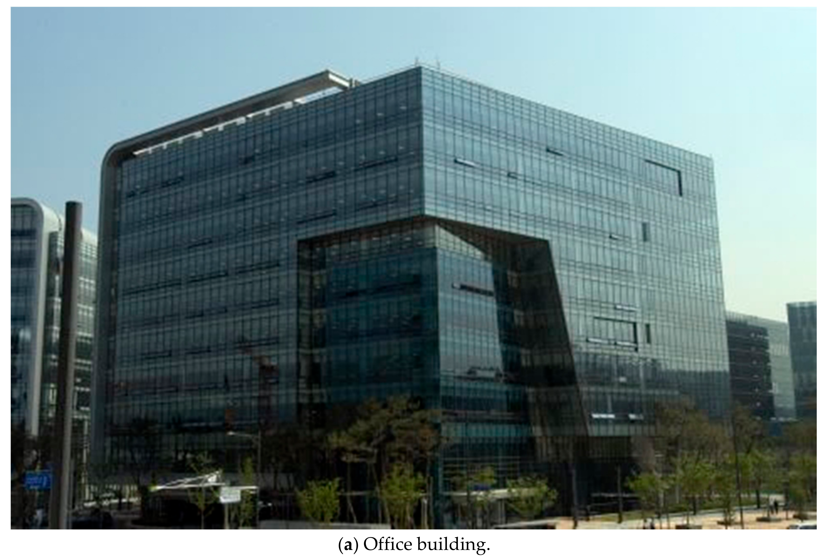

Figure 2.
The architecture of the inverse models for one-step ahead prediction.
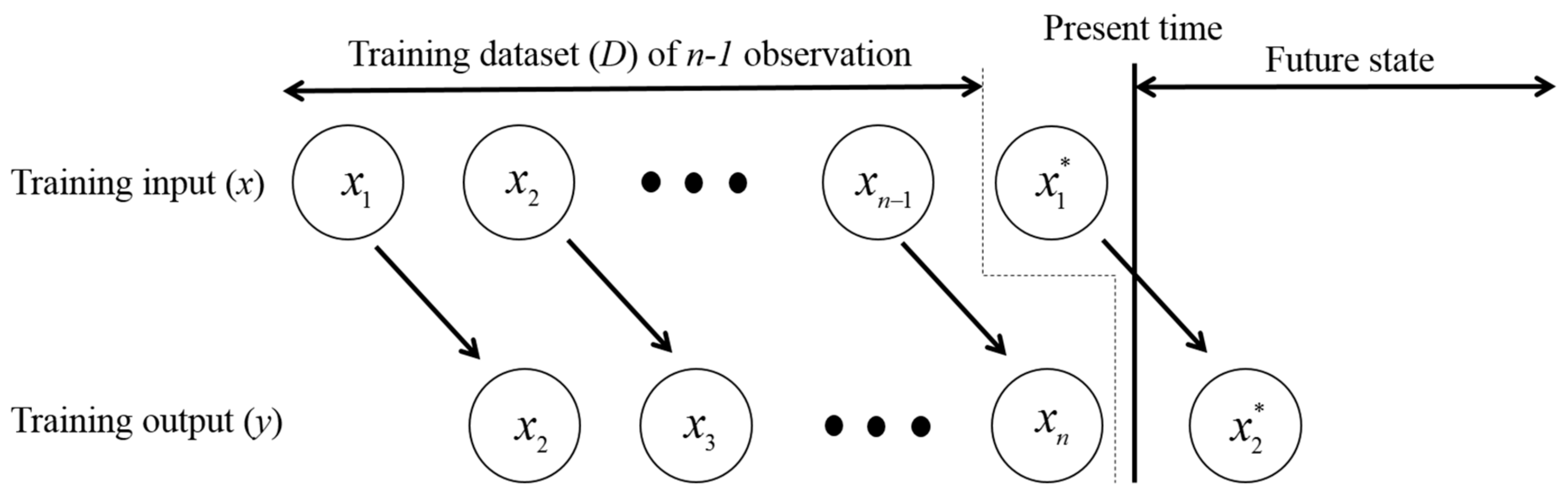
Figure 3.
Embedding dimension result using the False Nearest Neighbour (FNN) ratio.

Figure 4.
Time delay result using the Average Mutual Information (AMI).

Figure 5.
Three-dimensional phase space obtained from the BEMS data.

Figure 6.
Comparison between measured data and simulated outputs (SVR and Chaos SVR). SVR, Support Vector Regression.
Figure 6.
Comparison between measured data and simulated outputs (SVR and Chaos SVR). SVR, Support Vector Regression.


Table 1.
Comparison between SVR and Chaos SVR using Mean Bias Error (MBE) and Coefficient of Variance of the Root Mean Square Error (CVRMSE).
Table 1.
Comparison between SVR and Chaos SVR using Mean Bias Error (MBE) and Coefficient of Variance of the Root Mean Square Error (CVRMSE).
| k-Step | SVR | Chaos SVR | ||
|---|---|---|---|---|
| MBE | CVRMSE | MBE | CVRMSE | |
| 1-step | 4.85 | 12.26 | 4.13 | 13.75 |
| 2-step | 6.43 | 21.39 | 4.19 | 13.95 |
| 3-step | 8.32 | 31.33 | 4.20 | 13.97 |
| 4-step | 10.15 | 38.93 | 4.18 | 13.90 |
| 5-step | 10.87 | 43.08 | 4.18 | 13.90 |
| 6-step | 10.36 | 43.87 | 4.21 | 13.97 |
© 2017 by the author. Licensee MDPI, Basel, Switzerland. This article is an open access article distributed under the terms and conditions of the Creative Commons Attribution (CC BY) license (http://creativecommons.org/licenses/by/4.0/).
Share and Cite
MDPI and ACS Style
Kim, Y.-J. Comparison between Inverse Model and Chaos Time Series Inverse Model for Long-Term Prediction. Sustainability 2017, 9, 982. https://doi.org/10.3390/su9060982
AMA Style
Kim Y-J. Comparison between Inverse Model and Chaos Time Series Inverse Model for Long-Term Prediction. Sustainability. 2017; 9(6):982. https://doi.org/10.3390/su9060982
Chicago/Turabian StyleKim, Young-Jin. 2017. "Comparison between Inverse Model and Chaos Time Series Inverse Model for Long-Term Prediction" Sustainability 9, no. 6: 982. https://doi.org/10.3390/su9060982
Note that from the first issue of 2016, this journal uses article numbers instead of page numbers. See further details here.