
Optimal Weed Control Strategies in Rice Production under Dynamic and Static Decision Rules in South Korea

1
Department of Agricultural Economics and Rural Development, Seoul National University, Seoul 08826, Republic of Korea
2
Research Institute of Agriculture and Life Sciences, Seoul National University, Seoul 08826, Republic of Korea
*
Author to whom correspondence should be addressed.
Sustainability 2017, 9(6), 956; https://doi.org/10.3390/su9060956
Submission received: 31 March 2017
/
Revised: 30 May 2017
/
Accepted: 31 May 2017
/
Published: 12 June 2017
(This article belongs to the Section Environmental Sustainability and Applications)
Abstract
:This paper analyzes optimal weed control management strategies under static and dynamic decision rules. Seed bank is taken into account to introduce dynamics into the model. We present a numerical example of controlling Sheathed Monochoria (Monochoria Vaginalis) in Korean rice paddy fields. Our results show that producers benefit from dynamic decision rules; higher income and more control of weed density can be obtained with the same amount of herbicide. In order to illustrate the magnitude of differences between static and dynamic models, a numerical example is presented using a data set from Korean rice production. When it comes to controlling weed density, Korean rice farmers are found to be better off under the dynamic model, and the magnitude of advantages are found to be more sensitive to herbicide efficacy and less sensitive to initial seed banks and germination rates in terms of weed density.
1. Introduction
Herbicide is one of the major inputs in agricultural production, and has been credited with increasing productivity. Empirical literature on production risk and risk preferences has increased our knowledge on herbicide as an effective risk mitigation option, as it has been found to lower crop yield variability [1,2]. Pannell [3] argues that whether pesticide is a risk-reducing or a risk-increasing input is an empirical issue. When some sources of uncertainty (e.g., pest density, pesticide effectiveness) are taken into account, pesticides and herbicides can be considered as risk reducing inputs. However, the inappropriate use of herbicides has been raising concerns that it might be harmful to human health and the environment. Thus, it is important to establish optimal herbicide application rates and timing in order to abate the production risk, but at the same time, to minimize the possible damage to humans and the environment. This is also particularly pertinent to climate change adaptation, as global warming can drive the success of invasive plants like weeds [4].
Finding an economically efficient level of herbicide dosage requires the modelling of yield damage caused by weed crop competition. A rectangular hyperbola has been widely used to estimate the yield loss from weed crop competition [5]. Logistic functional form has been commonly used to describe a herbicide dose–response [6]. In crop science literature, research on farmers’ behavior of herbicide dosage has mostly focused on an economic threshold, deriving the herbicide dosage in order to keep crop yield losses below a certain level [7].
In economics literature, much attention has been devoted to establishing economic principles and policy implications of optimal weed control analysis using estimated biological functions. Wu [8] used seed bank as a state variable to develop a dynamic optimization model, and analyzed the differences between static and dynamic weed control strategies using Iowa corn production data as a numerical example. A discrete choice dynamic programming model was used to obtain the optimal composition of weed control options [9]. An input–output analysis was applied to evaluate the impacts of weeds on farm economy [10].
This study applies a dynamic programming model developed by Wu [8] to rice production data in South Korea, based on findings from crop science literature on rice (Oryza Sativa L.). Many studies on rice paddy weed control have mostly focused on the estimation of yield loss function and dose–response curve [11,12]. A cost–benefit analysis of herbicide dosage was conducted for rice farmers, deriving a threshold level to attain a certain level of weed density [13]. However, the analysis of the economic threshold ignores a profit maximization rule underlying producers’ behavior. In this regard, this paper tries to model a profit maximization principle in a dynamic setting and to provide an optimal level of herbicide dosage considering seed bank. We also compare the results from static and dynamic decision rules. Based on these efforts, this research attempts to develop policy implications towards an optimal weed control strategy. It is expected that valuable policy implications can be drawn in the sense that rice farmers are expected to be better off under a dynamic model, thus contributing to a sustainable rice economy.
2. Conceptual Framework
The following is a reformulation of a theoretical model suggested by Wu [8]. Assume that a typical rice farmer experiences yield losses due to an annual weed infestation. He/she considers an application of herbicides to maximize the sum of present values over T periods. The biological life cycle of annual rice weeds is comprised of four stages: germination, growth, interference, and seed production [14]. Some seeds buried in a rice paddy germinate in the spring, and the seedlings are exposed to some mortality factors such as frost, drought, herbivory, etc. Those who germinate after the first tillage grow up and compete with rice unless herbicides are applied in the fields. The seed density (hereafter, seed bank) at the very beginning of the farming season in year t is denoted by . Then, m portion of weed seeds are assumed to survive and compete with rice unless weed control measures are taken.
Farmers can control weeds in the fields by applying herbicides. The exponential functional form has been commonly used to describe dose–response relations [15]. Let denote herbicide dosage in year t. Then, the weed density competing with rice can be explained by , where c is a herbicide efficacy parameter taking a positive value depending on the weed species and herbicides used and m is a germination rate. Rice farmers can sustain the optimal weed density by controlling the herbicide dosage. Weeds that survive through some mortality factors can grow up, reproduce, and be spread by seeds, thereby completing a biological cycle. A new biological cycle begins again in the spring. Let k be the number of seeds that each weed produces. Then, a seed bank in the next year () can be calculated as .
The hyperbolic function is widely used to estimate yield losses from weed infestation [16,17]. Especially, an empirical model which is developed using rectangular hyperbola is most commonly used to predict yield damage from weed-crop competition [5,11,12,13,18,19]. In addition, we assume that yield losses take the form , where denotes the proportional yield losses given a certain level of weed density (W), and is a parameter measuring the magnitudes of weed-crop competition. When the weed density is , the yield loss rate is one-half. The yield response can be described as , where denotes weed-free rice yield.
In general, germination rate (m), herbicide efficacy (c), and weed-free crop () are subject to uncertainties such as temperature, rainfall, and other random factors. The role of uncertainty on weed control has been extensively examined in the crop science literature [2,15,20]. However, in order to focus solely on how farmers benefit from dynamic decision rules, we assume that these parameters are constant over time. Introducing uncertainty in this model would be a good topic for a future study.
Following Wu [8], profit maximization models under a dynamic setting can be written as
where is a discount factor, is the rice price in year t, is the herbicide price in year t, and denotes the cost of producing rice without considering the costs of herbicides. We assume that the state variable (=seed bank, ) changes throughout the state transition Equation (2), and an initial value of the state variable is given by (3).
The above discrete optimal control problem can be solved by Pontryagin’s maximum principle, which is widely used for finding an optimal path of control variables and corresponding state variables that maximize the objective function [21]. The associated Hamiltonian is given by , where the Lagrange Multiplier denotes the reduced value of maximized profit when one unit of seed bank increases. The first-order conditions for the Hamiltonian are given by
To see the role of control variables in the dynamic equilibrium, Equation (4) can be rewritten as
There are two outcomes of an increase in herbicides: firstly, the level of yield can be positively influenced by herbicide dosage; and secondly, seed bank in year decreases as weed density decreases in year t. The first term in Equation (7) denotes the discounted value of increased rice yield, and the second term reflects the decreased amount of seed banks in the next year multiplied by its shadow value. On the other hand, the RHS (right-hand-side) of Equation (7) denotes the present value of a unit price of herbicides. Thus, in a dynamic equilibrium, the marginal benefits of an extra unit of applied herbicide should be equal to its marginal cost, which is consistent with economic rationality in profit maximization.
To see the role of state variables in the dynamic equilibrium, Equation (5) can be rewritten as
Changes in seed bank in year t has two outcomes: firstly, yield in year t decreases as weed density in year t increases with ; secondly, seed bank in year also increases by the state transition Equation (2). The first term on the LHS (left-hand-side) of Equation (8) denotes the discounted damage of rice yields from increased seed bank in year t. The second term can be interpreted as an increased number of seed bank in year multiplied by its shadow value. The RHS of Equation (8) denotes the marginal cost of an extra unit of seed bank in year . Hence, in a dynamic equilibrium, the sum of discounted revenue reduction and the increased cost of seed bank in year should be equal to the marginal cost of the seed bank density of weeds in year .
Note that in order to derive the optimal path of weed density, Equation (4) can be rewritten as , where . (If we multiply Equation (5) by and add it to Equation (4), then we can get . It follows from the rectangular hyperbola damage function that . If we combine these with Equation (4), then we can get ). If and , then only the following solution meets the second order necessary condition:
In the last period, T, rice farmers only take into account the present profit. The optimal weed density in T () can be derived by inserting into Equation (9). Then, the optimal path of weed density can be obtained from Equation (9) and its corresponding seed bank. In this case, the optimal path of herbicide dosage can be derived as follows:
On the other hand, a model where farmers only consider the present profit can be alternatively written as , and the first-order condition is given by . The first-order condition can be rewritten as , where . If and , only the following positive solution meets the second-order necessary condition:
In this static world, the optimal path of weed density can be obtained, and its corresponding seed bank and herbicide dosage can be derived as follows:
In addition, the optimal weed seed bank under the dynamic decision rule is less than that of the static rule for the whole time horizon excluding the last period (T); that is, . is a decreasing function with respect to dt, and . Additionally, it follows that the number of optimal weed seed banks under the dynamic decision rule is smaller than that of the static decision ().
The sum of the present value of optimal profits over T periods can be calculated. Farmers under dynamic decision rules always get a weakly larger discounted sum of profits because they maximize net present value over all periods. Let and be the net present values under a dynamic decision rule and a static decision rule, respectively. The differences between the two terms are given by
3. Herbicide Application in Korean Rice Farming
Given the above conceptual model, we considered a case study of rice farming in South Korea as a numerical example. About 797,957 ha was used for rice cultivation in 2015, mostly located in the western part of the Korean peninsula (as shown in Figure 1).
According to a study done by Lee et al. [22], there are 433 weed species in Korean farmland, and about 77 species among those are present in rice paddy fields in South Korea. In the 1980’s, annual weeds like “Sheathed monochoria” (Monochoria vaginalis) and “Pygmy arrowhead” (Sagittaria pygmaea) were reported to be dominant [23]. As herbicides aimed at reducing annual weeds were developed, perennial weeds like “Water Chestnut” (Eleocharis kuroguwai Ohwi) and “Three-leaf arrowhead” (Sagittaria trifolia L.) increased [24]. In the 2000’s, herbicides to control perennial weeds were developed, and annual broadleaf weeds such as “Sheathed monochoria” and “Climbing seedbox” (Ludwigia prostrata) began to dominate [25,26]. As shown in Table 1, the importance value of Sheathed monochoria is the second highest among various weed species in South Korea. Importance value is the average of the relative frequency, relative density, and relative dominance of a weed [27]. This is an index of the dominance of a weed proposed by Curtis and Mcintosh [28]. Sheathed monochoria is among the top three most dominant weed species in western provinces, where most of rice production is concentrated [29].
Now, we provide a numerical example of optimal weed control strategies based on weed-crop competition between rice and “Sheathed monochoria”. We assume that Flucetosulfuron is considered as a measure of controlling “Sheathed monochoria”. Herbicide dosage, weed density, seed bank, and associated profits of rice farming are simulated under the optimal weed control model we presented in the previous section. Biological parameter estimates are needed to identify optimal weed control strategies under both dynamic and static settings.
Moon et al. [13] estimated weed-crop competitiveness (denoted by a parameter, ) and weed-free yield () in South Korea using a data set collected at Naju city. Spatial distributions of weed species were not considered because biological parameters for the analysis were only available for Naju city. According to this study, was and was equal to (ton/ha), which is assumed to be constant for all periods. Weed-free crop yields are generally subject to input choice, weather conditions, and technology. Thus, for accuracy, weed-free crop yields should be estimated based on these conditions. This paper uses estimates from Moon et al. [13], and assumes that the parameters remain unchanged for all periods. In Section 2, we assumed that the herbicide dose–response takes the form of exponential decay, but the log-logistic model is commonly used in the crop science field. Thus, we approximated the results from Moon et al. [30] using an exponential function, and herbicide efficacy (c) was approximated to be . The number of seeds produced by each weed (k) and germination rate (m) were taken from the Rural Development Administration in South Korea [31]. The number of initial seed bank per hectare is given by . When , . In this paper, we assume that initial seed bank results in 50 percent yield loss.
Next, rice price and cost parameters are summarized in Table 2.
Data on rice price are available in the Agriculture, Food and Rural Affairs Statistics Yearbook issued by MAFRA (Ministry of Agriculture, Food and Rural Affairs). Each year, MAFRA announces information on the government purchasing of rice for price stabilization. In this paper, government purchasing price of rice is used. The discount rate is assumed to be equal to 0.95 for all periods. The time horizon ranges from the year 2005 to the year 2009. Data of rice production costs can be obtained from Statistics Korea (National Statistical Office of Korea). In this study, we used cost information of Jeonnam province where Naju city is located and subtracted herbicide cost from the total cost. The unit cost of Flucetosulfuron was indirectly estimated based on some assumptions. This paper indirectly estimated the unit price of Flucetosulfuron by using herbicide costs per hectare from Moon et al. [13] and the herbicide guide from Kyungnong Corporation. We assume that farmers follow the user guide. The unit cost of herbicide application can be estimated from parameters given in the Table 3. We assume that unit cost of herbicides from 2006 to 2009 share the same trend with the total costs from the Agricultural Production Costs Survey from MAFRA (Republic of Korea) [32]. We also assume that there is no additional cost to applying herbicide in the fields.
4. Simulation Results
Optimal paths of herbicide application and weed seed bank under static and dynamic decision rules are summarized in Table 4. Once these paths have been revealed, the annual level of weed density and profits can be derived accordingly. As shown in Section 2, weed seed banks and weed density under a static decision rule were found to be higher than those under a dynamic decision rule. The weed density in the year 2009 was found to be 4.6178 (No./ha) under both of these alternative decision rules. This is because in the very last period, farmers under the dynamic decision rule behave as if there is no future to consider. We can also see that the herbicide dosage in the first period is much higher under the dynamic regime. The rice field is less likely to be infested with weeds if more herbicide is applied in the previous period, which consequently results in less weed seeds buried in the field. In other words, the reduction of weed density in the first period has a positive dynamic effect in terms of the shadow cost, since the optimal profit value decreases as the state variable weed seed bank increases. We found that the net present value was 1.97 (%) higher under a dynamic decision rule, which is consistent with the findings of Wu [8], who characterized the optimal reduction strategies of weeds such as Foxtail and Cocklebur in Iowa, USA.
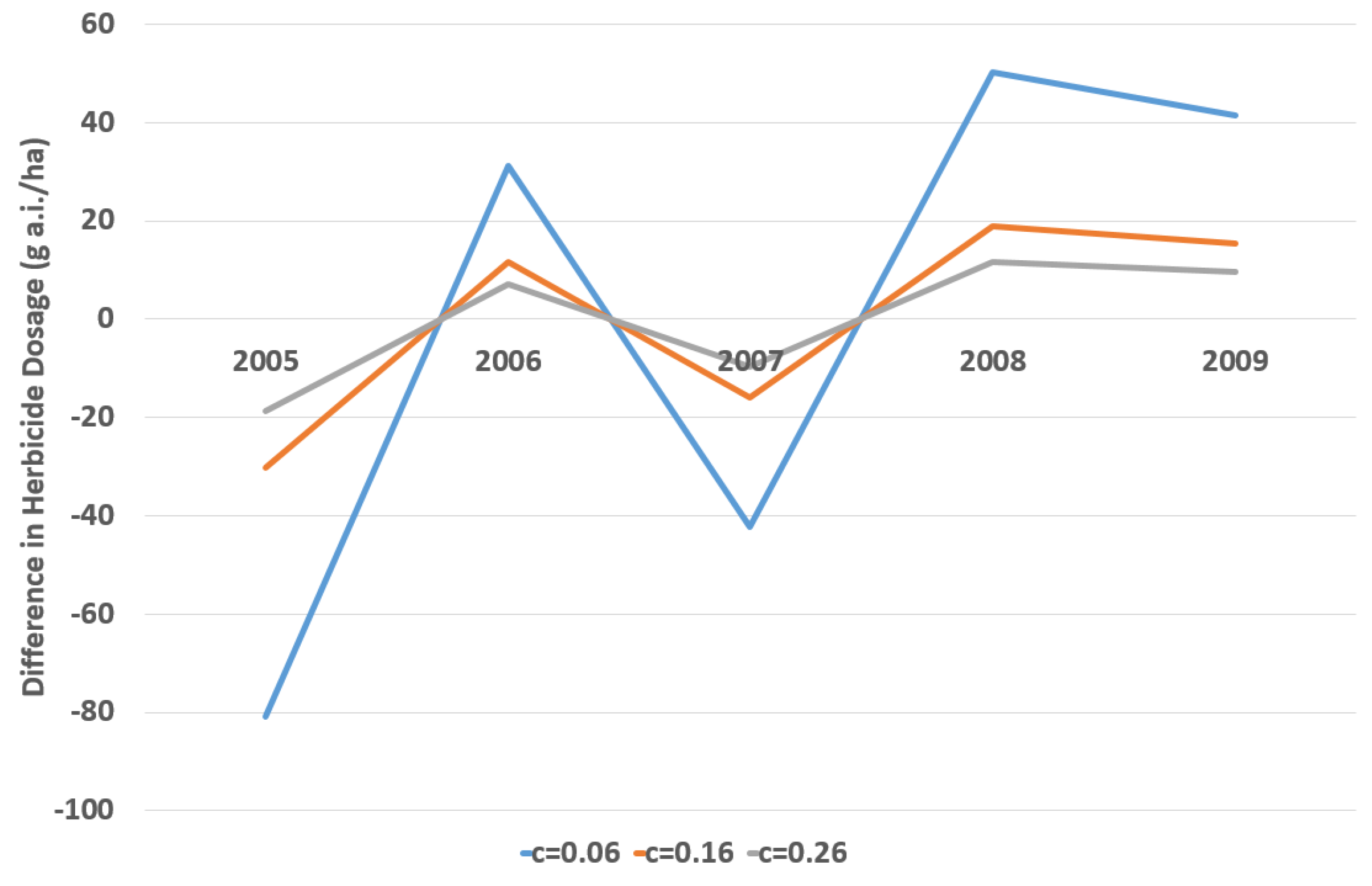
On the other hand, Pandey and Medd [35] found some empirical evidence that herbicide efficacy plays a key role in optimal weed control. Therefore, a sensitivity analysis is presented in this paper to see the effects of herbicide efficacy on farmers’ decisions. There are three scenarios in this sensitivity analysis. The baseline is such that herbicide efficacy (c) is equal to 0.16, where 80% of Sheathed monochoria can be removed if 10 g a.i. of Flucetosulfuron is applied in one hectare of rice paddy field. It follows from Table 5 and Figure 2 that differences in weed seed bank and weed density between two alternate decision regimes are much larger with less herbicide efficacy. For instance, if the efficacy decreases from 0.26 to 0.06, the difference of weed density in the first period increases from 2.7238 (No./ha) to 12.0005 (No./ha). The same result can be obtained in the difference of herbicide dosage as shown in Figure 3.
Initial seed bank () is considered as an important factor in weed control, and the level of initial seed bank varies depending on the conditions of the rice fields. An initial seed bank is assumed to be 56,523 (No./ha), which can result in about 50% yield loss when they germinate and survive without herbicide application. Table 6 shows the results under the new scenario where the initial seed bank is assumed to be 6280 (No./ha), which can result in about 10% yield loss.
The result of sensitivity analysis on the effect of initial seed bank shows that there is no great difference in optimal paths of control and state variables, except for herbicide dosage. The smaller the initial seed bank is, the less herbicide is applied in the first period, which makes more profits compared to the baseline scenario. Table 6 shows (along with Table 4) that the present value of total profits under dynamic decision increases by 51,366 (KRW/ha) compared to the baseline scenario. This means that the optimal time paths of herbicide dosage and profit after the first period are not very sensitive to the initial bank. Additionally, while there are differences in the total amount of herbicide usages and net present values, we found that there is not much difference in weed density at optimum between the two scenarios.
A germination rate (m) is also one of the critical factors in optimal weed control. Table 7 abbreviates the optimal time paths of some variables when the germination rate decreases from 2 to 1%.
This shows that when the germination rate decreases from 2 to 1%, net present value and total amount of herbicide applied under dynamic decision increase by 76,437 (KRW/ha) and 21.4615 (g a.i.), respectively, while annual differences in weed density are found to be the same. In this scenario, weed density between static and dynamic decisions are not same because of corner solution. Herbicide dosage can only take positive values.
5. Summary and Concluding Remarks
This paper applies an optimal weed control model developed by Wu [8] to Korean rice production data. Maximum principle is used to obtain the optimal path of control and state variables. Especially, reproduction of weed plants through seeds was considered to introduce dynamics in the model. A numerical example is presented with Sheathed monochoria, which has been reported to be dominant in the rice fields. The findings are summarized below.
First, even if a similar amount of herbicides is applied, a higher prevention effect and a larger amount of profits can be obtained under dynamic rules. Under dynamic regimes, farmers behave to maximize the net present value of profits, which makes them more profitable compared to static rules. Additionally, under dynamic rules, farmers use more herbicide in the first period, since they consider the transition of weed plants through seed banks and use less in the final period, because of low weed density attained by optimal dynamic planning. On the other hand, farmers with static decision rules do not consider seed bank dynamics, and therefore, the total amount of herbicide used will be similar. However, the prevention effect will be much lower, since seed bank dynamics were not considered in the decision-making process.
Second, the annual difference in weed density and weed seed bank is larger for the lower herbicide efficacy. Therefore, farmers will be more likely to be better off under dynamic decision rules if herbicide efficacy is low. However, differences in those variables are not sensitive to the initial seed bank () or germination rate (m).
Many studies have been carried out to describe yield loss from weed-crop competition and herbicide dose–response, which help us determine the optimal level of herbicide dosage [11,12,30]. Additionally, much research on finding the threshold of herbicide application to attain a certain level of weed density has been undertaken [13,18,19]. However, there is a huge research gap between this threshold analysis and reality because farmers do not take profit maximization principles into account. This paper attempted to analyze the optimal weed control under the profit maximization framework, incorporating research findings from crop science literature. In addition, gains from the dynamic decision rules were investigated over the static rules. These gains can be viewed as effective incentives for achieving sustainable rice production in South Korea.
The analysis in this paper has the following limitations: First, we have concentrated mainly on the effects of herbicide dosage on rice yields in both dynamic and static settings. Thus, price and yield uncertainties and farmers’ risk preferences were not incorporated into the model. Secondly, a spatial distribution of weed seed bank was not considered due to data limitations. These issues are good areas for future research.
Acknowledgments
This work was supported by the National Research Foundation of Korea-Grant funded by the Korean Government (NRF-2014S1A3A2044459).
Author Contributions
Woongchan Jeon and Kwansoo Kim conceived and developed the model. Woongchan Jeon and Kwansoo Kim analyzed results and wrote the manuscript. All authors have read and approved the final.
Conflicts of Interest
The authors declare no conflict of interest.
References
- Carlson, G.A. Risk reducing inputs related to agricultural pests. In Risk Analysis of Agricultural Firms: Concepts, Information Requirements and Policy Issues; Proceedings of Regional Research Project S-180; University of Illinois: Champaign, IL, USA, 1984; pp. 164–175. [Google Scholar]
- Feder, G. Pesticides, information, and pest management under uncertainty. Am. J. Agric. Econ. 1979, 61, 97–103. [Google Scholar] [CrossRef]
- Pannell, D.J. Pests and pesticides, risk and risk aversion. Agric. Econ. 1991, 5, 361–383. [Google Scholar] [CrossRef]
- Vila, M.; Corbin, J.D.; Dukes, J.S.; Pino, J.; Smith, S.D. Linking plant invasions to global environmental change. In Terrestrial Ecosystems in a Changing World; Canadell, J.G., DPataki, D.E., Pitelka, L.F., Eds.; Springer: Heidelberg, Germany, 2007; pp. 93–102. [Google Scholar]
- Cousens, R. A simple model relating yield loss to weed density. Ann. Appl. Biol. 1985, 107, 239–252. [Google Scholar] [CrossRef]
- Streibig, J. Models for curve-fitting herbicide dose response data. Acta Agric. Scand. 1980, 30, 59–64. [Google Scholar] [CrossRef]
- Kim, D.; Brain, P.; Marshall, E.; Caseley, J. Modelling herbicide dose and weed density effects on crop: Weed competition. Weed Res. 2002, 42, 1–13. [Google Scholar] [CrossRef]
- Wu, J. Optimal weed control under static and dynamic decision rules. Agric. Econ. 2000, 25, 119–130. [Google Scholar] [CrossRef]
- Odom, D.I.; Cacho, O.J.; Sinden, J.; Griffith, G.R. Policies for the management of weeds in natural ecosystems: The case of scotch broom (Cytisus scoparius L.) in an Australian national park. Ecol. Econ. 2003, 44, 119–135. [Google Scholar] [CrossRef]
- Eiswerth, M.E.; Darden, T.D.; Johnson, W.S.; Agapoff, J.; Harris, T.R. Input–output modeling, outdoor recreation, and the economic impacts of weeds. Weed Sci. 2005, 53, 130–137. [Google Scholar] [CrossRef]
- Lee, S.-G.; Kim, D.-S.; Im, I.-B.; Pyon, J.-Y. Growth and yield of rice as affected by different densities of perennial weeds and prediction of rice yield loss in paddy fields. Korean J. Weed Sci. 2005, 25, 295–303. [Google Scholar]
- Song, S.-B.; Hong, Y.-G.; Hwang, J.-B.; Park, S.-T.; Kim, H.-Y. Loss of rice growth and yield affected by weed competition in machine transplanted rice cultivation. Korean J. Weed Sci. 2006, 26, 407–412. [Google Scholar]
- Moon, B.-C.; Kwon, O.-D.; Cho, S.-H.; Lee, S.-G.; Won, J.-G.; Lee, I.-Y.; Park, J.-E.; Kim, D.-S. Modeling the Competition Effect of Sagittaria trifolia and Monochoria vaginalis Weed Density on Rice in Transplanted Rice Cultivation. Korean J. Weed Sci. 2012, 32, 188–194. [Google Scholar] [CrossRef]
- Bauer, T.A.; Mortensen, D.A. A comparison of economic and economic optimum thresholds for two annual weeds in soybeans. Weed Technol. 1992, 6, 228–235. [Google Scholar]
- Deen, W.; Weersink, A.; Turvey, C.; Weaver, S. Economics of weed control strategies under uncertainty. Rev. Agric. Econ. 1993, 15, 39–50. [Google Scholar] [CrossRef]
- Coble, H.D.; Mortensen, D.A. The threshold concept and its application to weed science. Weed Technol. 1992, 6, 191–195. [Google Scholar]
- Wilkerson, G.; Modena, S.; Coble, H. HERB: Decision model for postemergence weed control in soybean. Agron. J. 1991, 83, 413–417. [Google Scholar] [CrossRef]
- Al Mamun, M.A. Modelling rice-weed competition in direct-seeded rice cultivation. Agric. Res. 2014, 3, 346–352. [Google Scholar] [CrossRef]
- Moon, B.-C.; Cho, S.-H.; Kwon, O.-D.; Lee, S.-G.; Lee, B.-W. Modelling rice competition with Echinochloa crus-galli and Eleocharis kuroguwai in transplanted rice cultivation. J. Crop Sci. Biotechnol. 2010, 13, 121–126. [Google Scholar] [CrossRef]
- Swinton, S.M.; King, R.P. The value of pest information in a dynamic setting: The case of weed control. Am. J. Agric. Econ. 1994, 76, 36–46. [Google Scholar] [CrossRef]
- Pontryagin, L.S. Mathematical Theory of Optimal Processes; Gordon and Breach Sceince Publishers S.A.: New York, NY, USA, 1986. [Google Scholar]
- Lee, I.-Y.; Park, J.-E.; Kim, C.-S.; Oh, S.-M.; Chung-Kil, K.; Park, T.-S.; Cho, J.-R.; Moon, B.-C.; Kwon, O.-S.; Kim, K.-H.; et al. Characteristics of weed flora in arable land of Korea. Korean J. Weed Sci. 2007, 27, 1–21. [Google Scholar]
- Oh, Y.; Ku, Y.; Lee, J.; Ham, Y. Distribution of weed population in the paddy field in Korea, 1981. Korean J. Weed Sci. 1981, 1, 21–29. [Google Scholar]
- Park, K.; Oh, Y.; Ku, Y.; Kim, H.; Sa, J.; Park, J.; Kim, H.; Kwon, S.; Shin, H.; Kim, S. Changes of weed community in lowland rice field [s] in Korea. Korean J. Weed Sci. 1995, 15, 254–261. [Google Scholar]
- Park, J.-S.; Cho, Y.-C.; Han, S.-W.; Lim, G.J.; Lee, W.W.; Ju, Y.C.; Kim, Y.H. Weed population distribution and change of dominant weed species on paddy field in Kyonggi region. Korean J. Weed Sci. 2001, 21, 320–326. [Google Scholar]
- Park, J.-S.; Kim, H.-D.; Han, S.-W.; Lee, J.-H.; Jang, J.-H. Weed population distribution and change of dominant weed species in paddy field of Gyeonggi region. Korean J. Weed Sci. 2007, 27, 56–65. [Google Scholar] [CrossRef]
- Kershaw, K.A. Quantitative and Dynamic Plant Ecology, 2nd ed.; American Elsevier Pub. Co.: New York, NY, USA, 1964. [Google Scholar]
- Curtis, J.T.; McIntosh, R.P. The interrelations of certain analytic and synthetic phytosociological characters. Ecology 1950, 31, 434–455. [Google Scholar] [CrossRef]
- Ha, H.-Y.; Hwang, K.S.; Suh, S.J.; Lee, I.-Y.; Oh, Y.-J.; Park, J.; Choi, J.-K.; Kim, E.J.; Cho, S.H.; Kwon, O.-D. A survey of weed occurrence on paddy field in Korea. Weed Turfgrass Sci. 2014, 3, 71–77. [Google Scholar] [CrossRef]
- Moon, B.-C.; Kim, J.-W.; Cho, S.-H.; Park, J.-E.; Song, J.-S.; Kim, D.-S. Modelling the effects of herbicide dose and weed density on rice–weed competition. Weed Res. 2014, 54, 484–491. [Google Scholar] [CrossRef]
- Nongsaro. Available online: www.nongsaro.go.kr/portal/Main.ps?menuId=PS00001(accessed on 27 March 2017).
- Korean Statistical Information Service (KOSIS). Available online: kosis.kr/statisticsList/statisticsList_01List.jsp?vwcd=MT_ZTITLE&parentIdF (accessed on 27 March 2017).
- Korea National Index. Available online: www.index.go.kr/index.jsp?oid=N (accessed on 27 March 2017).
- Korea Crop Protection Association. Available online: koreacpa.org/index3/main.php (accessed on 27 March 2017).
- Pandey, S.; Medd, R.W. A stochastic dynamic programming framework for weed control decision making: An application to Avena fatua L. Agric. Econ. 1991, 6, 115–128. [Google Scholar] [CrossRef]
Figure 1.
Rice cultivation area (ha)/County in South Korea.
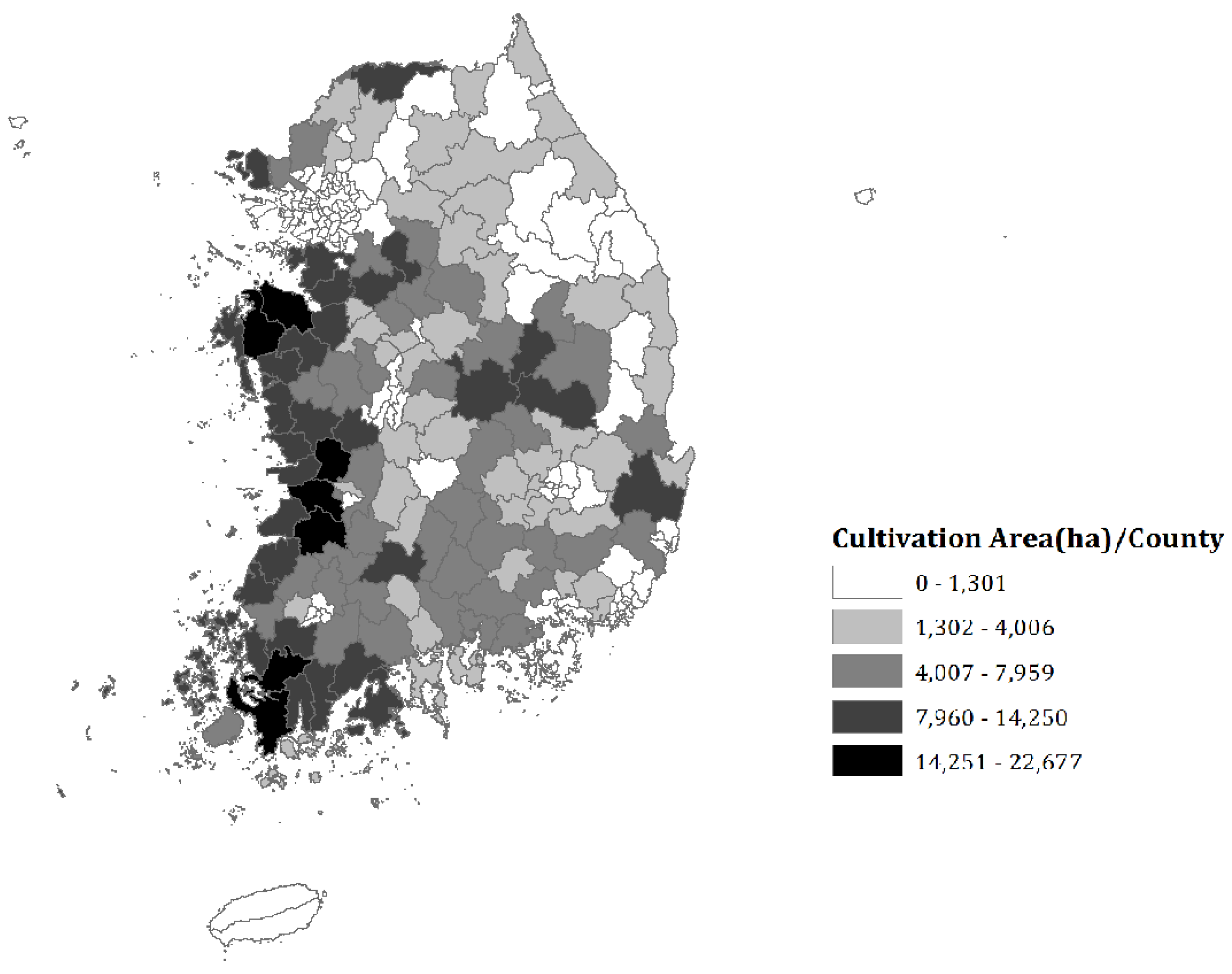
Figure 2.
Differences in weed density under dynamic and static decision rules.
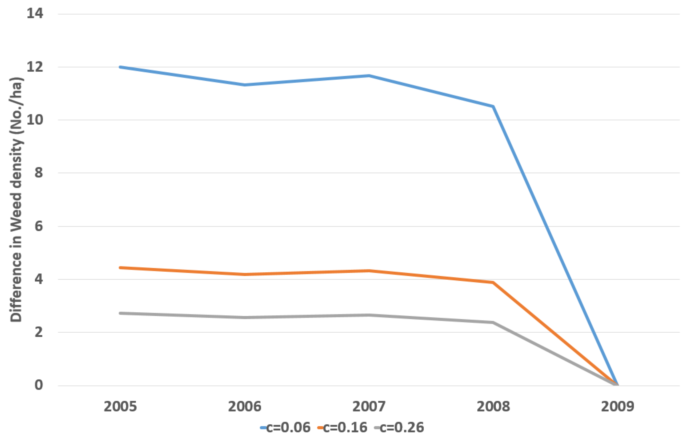
Figure 3.
Differences in herbicide dosage under dynamic and static decision rules.

Table 1.
Top 10 weed species in direct-seeding rice paddy fields in South Korea.
| Rank | Species | Importance Value |
|---|---|---|
| 1 | Echinochloa spp. | 23.0 |
| 2 | Monochoria vaginalis | 14.1 |
| 3 | Aeschynomene indica | 5.5 |
| 4 | Ludwigia prostrata | 4.8 |
| 5 | Scirpus juncoides | 4.6 |
| 6 | Cyperus difformis | 4.4 |
| 7 | Aneilema keisak | 4.8 |
| 8 | Eclipta prostrata | 4.2 |
| 9 | Bidens frondosa | 3.5 |
| 10 | Eleocharis kuroguwai | 4.2 |
Data: Ha et al. [29].
Table 2.
Annual rice price in South Korea and annual production costs of rice in Jeonnam province.
| 2005 | 2006 | 2007 | 2008 | 2009 | |
|---|---|---|---|---|---|
| Price (KRW/t) | 1,211,250 | 1,281,750 | 1,300,750 | 1,410,750 | 1,234,750 |
| Herbicide price (KRW/g a.i.) | 3937 | 4111 | 4282 | 4728 | 4971 |
| Costs excluding herbicides (KRW/ha) | 5,356,490 | 5,592,410 | 5,579,410 | 5,914,640 | 5,632,450 |
Note: g a.i. = gram active ingredients.
Table 3.
Unitary costs of applying Flucetosulfuron.
| (A) | (B) | (C) | (D) |
|---|---|---|---|
| Herbicide Costs | Exchange Rate in 2005 | Recommended Dosage | Unit Cost of Herbicide Application |
| ($/10a) | (KRW/$) | (g a.i./10a) | (KRW/g) |
| 9.73 | 1011.6 | 2.5 | 3937 |
Table 4.
Optimal paths of seed bank, weed density, herbicide application, and profits under dynamic and static decisions.
Table 4.
Optimal paths of seed bank, weed density, herbicide application, and profits under dynamic and static decisions.
| Year | A Static Model | A Dynamic Model | ||||||
|---|---|---|---|---|---|---|---|---|
| Seed Bank | Weed Density | Herbicide | Profit | Seed Bank | Weed Density | Herbicide | Profit | |
| (No./ha) | (No./ha) | (g a.i./ha) | (KRW */ha) | (No./ha) | (No./ha) | (g a.i./ha) | (KRW/ha) | |
| 2005 | 56,523.0000 | 4.4755 | 34.5736 | 747,270 | 56,523.0000 | 0.0356 | 64.7888 | 652,815 |
| 2006 | 4475.4650 | 4.4158 | 18.8073 | 933,699 | 35.5850 | 0.2293 | 7.0792 | 1,006,357 |
| 2007 | 4415.7550 | 4.3401 | 18.8313 | 1,045,112 | 229.2909 | 0.0177 | 34.7199 | 1,005,577 |
| 2008 | 4340.0910 | 4.2410 | 18.8677 | 1,272,463 | 17.7349 | 0.3547 | 0.0000 | 1,379,470 |
| 2009 | 4240.9840 | 4.6178 | 18.1913 | 652,385 | 354.6971 | 4.6178 | 2.6832 | 716,588 |
| Total | 73,995.2950 | 22.0901 | 109.2712 | 4,650,928 | 57,160.3080 | 5.2551 | 109.2712 | 4,760,807 |
| (PV) | (3,989,854) | (4,068,637) | ||||||
Note: 1$ = 1,114 KRW (Korean Won) as of 28 March 2017; PV= present value.
Table 5.
Sensitivity analysis of herbicide efficacy.
| Year | Differences in Weed Density | Differences in Herbicide Dosage | ||||
|---|---|---|---|---|---|---|
| under Static and Dynamic | under Static and Dynamic | |||||
| Decisions (No./ha) | Decisions (g a.i./ha) | |||||
| c = 0.06 | c = 0.16 | c = 0.26 | c = 0.06 | c = 0.16 | c = 0.26 | |
| 2005 | 12.0005 | 4.4399 | 2.7238 | −80.7953 | −30.2153 | −18.5824 |
| 2006 | 11.3200 | 4.1865 | 2.5681 | 31.2875 | 11.7281 | 7.2166 |
| 2007 | 11.6774 | 4.3224 | 2.6520 | −42.3604 | −15.8886 | −9.7781 |
| 2008 | 10.5067 | 3.8863 | 2.3841 | 50.3189 | 18.8677 | 11.6106 |
| 2009 | 0 | 0 | 0 | 41.5493 | 15.5080 | 9.5332 |
Table 6.
Optimal paths of seed bank, weed density, herbicide application, and profits under dynamic and static decision rules when is assumed to be 6,280 (No./ha).
Table 6.
Optimal paths of seed bank, weed density, herbicide application, and profits under dynamic and static decision rules when is assumed to be 6,280 (No./ha).
| A Static Model | A Dynamic Model | |||||||
|---|---|---|---|---|---|---|---|---|
| Year | Seed Bank | Weed Density | Herbicide | Profit | Seed Bank | Weed Density | Herbicide | Profit |
| (No./ha) | (No./ha) | (g a.i./ha) | (KRW/ha) | (No./ha) | (No./ha) | (g a.i./ha) | (KRW/ha) | |
| 2005 | 6280.0000 | 4.4755 | 20.8406 | 801,339 | 6280.0000 | 0.0356 | 51.0558 | 706,884 |
| 2006 | 4475.4650 | 4.4158 | 18.8073 | 933,699 | 35.5850 | 0.2293 | 7.0792 | 1,006,357 |
| 2007 | 4415.7550 | 4.3401 | 18.8313 | 1,045,112 | 229.2909 | 0.0177 | 34.7199 | 1,005,577 |
| 2008 | 4340.0910 | 4.2410 | 18.8677 | 1,272,463 | 17.7349 | 0.3547 | 0.0000 | 1,379,470 |
| 2009 | 4240.9840 | 4.6178 | 18.1913 | 652,385 | 354.6971 | 4.6178 | 2.6832 | 716,588 |
| Total | 23,752.2950 | 22.0901 | 95.5382 | 4,704,997 | 6917.3080 | 5.2551 | 95.5382 | 4,814,876 |
| (PV) | (4,041,220) | (4,120,003) | ||||||
Table 7.
Optimal paths of seed bank, weed density, herbicide application, and profits under dynamic and static decision rules when m is assumed to be 0.01.
Table 7.
Optimal paths of seed bank, weed density, herbicide application, and profits under dynamic and static decision rules when m is assumed to be 0.01.
| A Static Model | A Dynamic Model | |||||||
|---|---|---|---|---|---|---|---|---|
| Year | Seed Bank | Weed Density | Herbicide | Profit | Seed Bank | Weed Density | Herbicide | Profit |
| (No./ha) | (No./ha) | (g a.i./ha) | (KRW/ha) | (No./ha) | (No./ha) | (g a.i./ha) | (KRW/ha) | |
| 2005 | 56,523.0000 | 4.4755 | 30.2414 | 764,327 | 56,523.0000 | 0.0356 | 60.4566 | 669,871 |
| 2006 | 4475.4650 | 4.4158 | 14.4751 | 951,506 | 35.5850 | 0.2293 | 2.7470 | 1,024,165 |
| 2007 | 4415.7550 | 4.3401 | 14.4992 | 1,062,878 | 229.2909 | 0.0447 | 24.6061 | 1,046,893 |
| 2008 | 4340.0910 | 4.2410 | 14.5355 | 1,291,297 | 44.7281 | 0.4473 | 0.0000 | 1,378,873 |
| 2009 | 4240.9840 | 4.6178 | 13.8591 | 670,320 | 447.2811 | 4.4728 | 0.0000 | 728,509 |
| Total | 73,995.2950 | 22.0901 | 87.6103 | 4,740,327 | 57,279.8852 | 5.2297 | 87.8097 | 4,848,312 |
| (PV) | (4,066,580) | (4,145,074) | ||||||
© 2017 by the authors. Licensee MDPI, Basel, Switzerland. This article is an open access article distributed under the terms and conditions of the Creative Commons Attribution (CC BY) license (http://creativecommons.org/licenses/by/4.0/).
Share and Cite
MDPI and ACS Style
Jeon, W.; Kim, K. Optimal Weed Control Strategies in Rice Production under Dynamic and Static Decision Rules in South Korea. Sustainability 2017, 9, 956. https://doi.org/10.3390/su9060956
AMA Style
Jeon W, Kim K. Optimal Weed Control Strategies in Rice Production under Dynamic and Static Decision Rules in South Korea. Sustainability. 2017; 9(6):956. https://doi.org/10.3390/su9060956
Chicago/Turabian StyleJeon, Woongchan, and Kwansoo Kim. 2017. "Optimal Weed Control Strategies in Rice Production under Dynamic and Static Decision Rules in South Korea" Sustainability 9, no. 6: 956. https://doi.org/10.3390/su9060956
Note that from the first issue of 2016, this journal uses article numbers instead of page numbers. See further details here.