Article

Hybrid Algorithm Based on an Estimation of Distribution Algorithm and Cuckoo Search for the No Idle Permutation Flow Shop Scheduling Problem with the Total Tardiness Criterion Minimization

Key Laboratory of Advanced Control and Optimization for Chemical Process, East China University of Science and Technology, Ministry of Education, Shanghai 200237, China
*
Author to whom correspondence should be addressed.
Sustainability 2017, 9(6), 953; https://doi.org/10.3390/su9060953
Submission received: 30 April 2017 / Revised: 29 May 2017 / Accepted: 1 June 2017 / Published: 5 June 2017

Abstract

:
The no idle permutation flow shop scheduling problem (NIPFSP) is a popular NP-hard combinatorial optimization problem, which exists in several real world production processes. This study proposes a novel hybrid estimation of the distribution algorithm and cuckoo search (CS) algorithm (HEDA_CS) to solve the NIPFSP with the total tardiness criterion minimization. The problem model is built on the basis of the starting and ending time point of each job. A discrete solution representation method is applied in HEDA_CS to increase the operation efficiency. A novel probability matrix build method is also designed within the knowledge of the processing time matrix. The partially-mapped crossover operation works effectively during the CS phase. A suitable knowledge-based local search is also designed in the HEDA_CS to balance the exploitation and exploration. Finally, many simulations based on the new hard Ruiz benchmarks are conducted. Computational results demonstrate the effectiveness of the proposed HEDA_CS.

1. Introduction

The permutation flow shop scheduling problem (PFSP) has been the focus of many studies for decades. The no-idle constraint in scheduling occurs when two consecutive jobs must be processed on the same machine without any interruptions. Given that this constraint appears in real-world production environments, the no idle permutation flow shop scheduling problem (NIPFSP) has considerable academic and practical significance. Similar to the traditional scheduling problem, the NIPFSP is proven to be NP-hard [1,2]. Exact optimization methods have limitations in solving large-scale problems because of the calculation time limitation. Therefore, developing effective and efficient algorithms to solve the NIPFSP is significant.
The NIPFSP was first studied by Adiri and Pohoryles [3], and it has received extensive attention ever since. Woollam [4] investigated a solution procedure for a flow shop problem, in which a machine continuously processes all the jobs that must be processed once it is started. That study described a “no idle time allowed” constraint. Saadani et al. [5] determined that the idle characteristic seriously affected the value of the makespan (Cmax) criterion in a three-stage, no idle flow-shop configuration. Given that the traditional exact optimization algorithm has limitations with the age of data exploration, heuristics has received increasing attention by solving the NIPFSP [6,7,8,9,10]. Dong et al. [11] proposed an improved NEH-based heuristic with an initial sequence generated by combining the average job processing time. Their proposed strategy was based on the idea of balancing the utilization among all machines and exhibited suitable performance. Baraz and Mosheiov [12] introduced an efficient (O(n2)) greedy algorithm, which was shown numerically to perform better than other published heuristics. Kalczynski and Kamburowski [13] addressed the problem of determining a job sequence that minimized the makespan in m-machine flow shops under the no-idle condition. Pan and Wang [14] proposed a novel discrete differential evolution algorithm to solve NIPFSP. That study presented two simple approaches to calculate the makespan and a speed-up method to insert the neighborhood and thus improve the efficiency of the entire algorithm. Pan et al. [15] then proposed a new and novel referenced local search procedure hybridized with both algorithms to further improve the solution quality. The referenced local search exploited the space based on reference positions taken from a reference solution to determine better job positions when performing the insertion operation. Researchers [16] also solved the single machine total weighted tardiness problem with sequence dependent setup times by a discrete differential evolution algorithm. He and Wang [17] proposed a hybrid algorithm that combines evolutionary computation and constraint-handling techniques. Li and Wang [18] proposed a hybrid quantum-inspired genetic algorithm for the multi-objective PFSP. A new random-key representation was used to convert the Q-bit representation to job permutation in evaluating the objective values of the schedule solution. Deng and Gu [19] proposed a hybrid discrete differential evolution (HDDE) algorithm for the no-idle permutation flow shop scheduling problem with makespan criterion. Tasgetiren et al. [20] investigated the utilization of a continuous algorithm for the NIPFSP with tardiness criterion. A differential evolution algorithm with variable parameter search was developed to solve the NIPFSP. Researchers [21] also designed a variable iterated greedy algorithm with differential evolution to solve the NIPFSP in recent years. Pan and Ruiz [22] first proposed an effective iterated greedy algorithm for a mixed no idle flow shop, where several machines had the no-idle constraint, whereas others were regular machines. The researchers also proposed a formula set to accelerate the insertion calculation that was utilized in heuristics and in local search procedures. A novel nature-inspired cuckoo search (CS) algorithm was developed by Yang and Deb [23] in 2009. CS has a series of successful engineering examples [24,25,26]. The improved CS algorithm was proposed for hybrid flow shop scheduling problems by Marichelvam et al. [27], and the algorithm was validated with the data from a leading furniture manufacturing company. A discrete version of the inter-species CS algorithm was proposed and applied to solve two significant types of the PFSP [28].
The current study is related to the complex production process with no idle tight constraints in the real world. Given that the starting and ending time points are a suitable method to describe the job process, a new problem formulation is built on the basis of this condition. Considering the last CS algorithm, this study proposes a novel hybrid estimation of distribution algorithm (HEDA) and CS algorithm (HEDA_CS) to solve the NIPFFSP with the total tardiness criterion minimization. A knowledge-based local search is applied to the proposed HEDA_CS to balance the exploitation and exploration of the HEDA_CS. Several latest Ruiz benchmark instances are adopted to test and improve the HEDA_CS performance. A suitable adjustment to the algorithm shows that the HEDA_CS is effective and highly efficient in solving the NIPFFSP with the total tardiness criterion minimization.
The remainder of the paper is organized as follows. Section 2 describes the problem formulation with a time point method to build the mathematical model. Section 3 presents the novel HEDA_CS to solve the NIPFSP with the total tardiness criterion minimization. Several of the latest Ruiz benchmark instances are employed to test the performance of the proposed HEDA_CS in Section 4. The computational results and analysis are also presented in this section. Finally, the conclusions are discussed in Section 5.

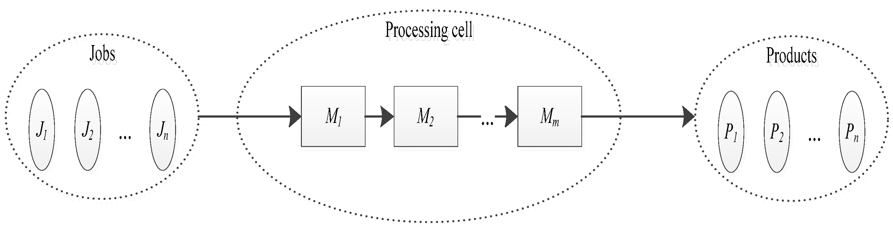
2. Problem Formulation

The permutation flow shop scheduling problem (PFSP) is illustrated in Figure 1. A total of n jobs J = {J1, J2, , Ji, , Jn−1, Jn} must be processed on m machines M = {M1, M2, , Mj, , Mm−1, Mm} with the same sequence. Consequently, n products {P1, P2, , Pi, , Pn−1, Pn} are attained. Therefore, determining the processing sequence of n jobs over m machines in PFSP to satisfy several objectives is widely applied in actual production, especially in one-piece mass production. The NIPFSP is a highly important branch of PFSP and an NP-hard problem. Additional mathematical descriptions are presented in the following subsections.

2.1. Notation

i, jnormally utilized as loop variables (i.e., i represents the job number, and j represents the machine number)
mmachine number
njob number
Job{J1, J2, ….., Jn}; represents the job set to be processed
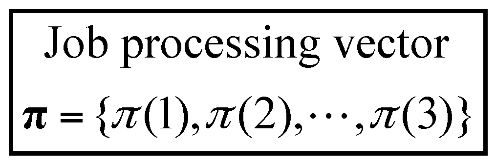
πscheduling solution that is the processing sequence of the job set {J1, J2, ….., Jn}
Ti,jrepresents the processing time of the i-th job processed on the j-th machine
Tsi,jrepresents the starting time of the i-th processed job on the j-th machine;
Given that all of the jobs are prepared to be processed at time zero, then T s π ( 1 ) , 1 = 0
Tei,jrepresents the ending time of the i-th processed job on the j-th machine
DifTi,jrepresents the minimum difference time between the π(i)-th processed job completion time of the j-th machine and (j + 1)-th machine
direpresents the due date of the i-th job
T T d ( π ) represents the total tardiness of the schedule π

2.2. Mathematical Model

The NIPFSP has the same requirements (i.e., processing sequence) as the PFSP [2,5,14]. In particular, n jobs must be processed on m machines with the same sequence. Each machine can only process one job at a time. No interruption occurs between the start and end of each job, and all of the jobs are prepared to be processed at time zero. However, a significant difference exists between the two problems. The NIPFSP has tight time constraints for each machine. In particular, each machine must process all of the jobs without any interruption from the start of processing the first job to the end of the last job. The total tardiness (TTd) of the NIPFSP for this feature can be calculated as follows:
min   T T d ( π )
f i r s t   m a c h i n e : T s π ( 1 ) , 1 = 0 T e π ( 1 ) , 1 = T s π ( 1 ) , 1 + T π ( 1 ) , 1 = T π ( 1 ) , 1 T e π ( i ) , j = T s π ( i ) , j + T π ( i ) , j T s π ( i ) , j + 1 T e π ( i ) , j T s π ( i ) , 1 = T e π ( i 1 ) , 1 ( 2 i n ; i N + ) T e π ( i ) , 1 = T e π ( i 1 ) , 1 + T π ( i ) , 1 f o l l o w i n g   m a c h i n e s : D i f T 1 , j = T π ( 1 ) , j + 1 , j = 1 , 2 , , m 1 D i f T i , j = max { 0 , D i f T i 1 , j T π ( i ) , j } + T π ( i ) , j + 1 ( 1 < i n ; 1 j < m ; i , j N + ) T e π ( n ) , j = j j = 1 j 1 D i f T n , j j + i = 1 n T π ( i ) , 1 ( 2 j m , j N + ) T s π ( i ) , j = T e π ( i ) , j T π ( i ) , j = T e π ( i 1 ) , j ( 2 i n ; 1 j m ; i , j N + ) T T d ( π ) = i = 1 n T T d π ( i ) = i = 1 n max { T e π ( i ) , m d π ( i ) , 0 }
The aforementioned equations describe the processing sequence through the variables TS and TE. The relationship between TS and TE shows no idle tight time constraints. Therefore, several jobs must be processed with time delay when they are free from several machines. The variable DifTi,j is employed to ensure the exact delay time. The ending time of the last processed job at each machine can be calculated through the sum DifTi,j with Ti,j. The ending time of each job at the last machine can then be attained by forward pass calculation. Finally, the total tardiness of the schedule π can be obtained. The objective of solving NIPFSP is to determine a suitable solution (i.e., π) with the total tardiness T T d ( π ) minimization. An example of the NIPFSP problem with five jobs and three machines is shown in Figure 2 in describing the manufacturing process. The five jobs are processed on the three machines with the same job process vector [4 1 5 3 2]. The no idle constraint exists, whether the jobs are processed on the first machine or the following machines. The starting time and end time of each job are also posted in Figure 2.

3. HEDA_CS for NIPFSP

Significant applications of hybrid algorithms to solve scheduling problems with suitable performance have been explored in the past few decades [29,30,31,32]. This section presents the novel HEDA_CS for solving the NIPFSP with the total tardiness minimization. First, a discrete vector solution representation and initialization with the building probability model is introduced. Second, a hybrid strategy with CS, updating mechanism, and knowledge-based local search are described in detail. Finally, the flowchart of the HEDA_CS is shown to better understand the circulation mechanism.

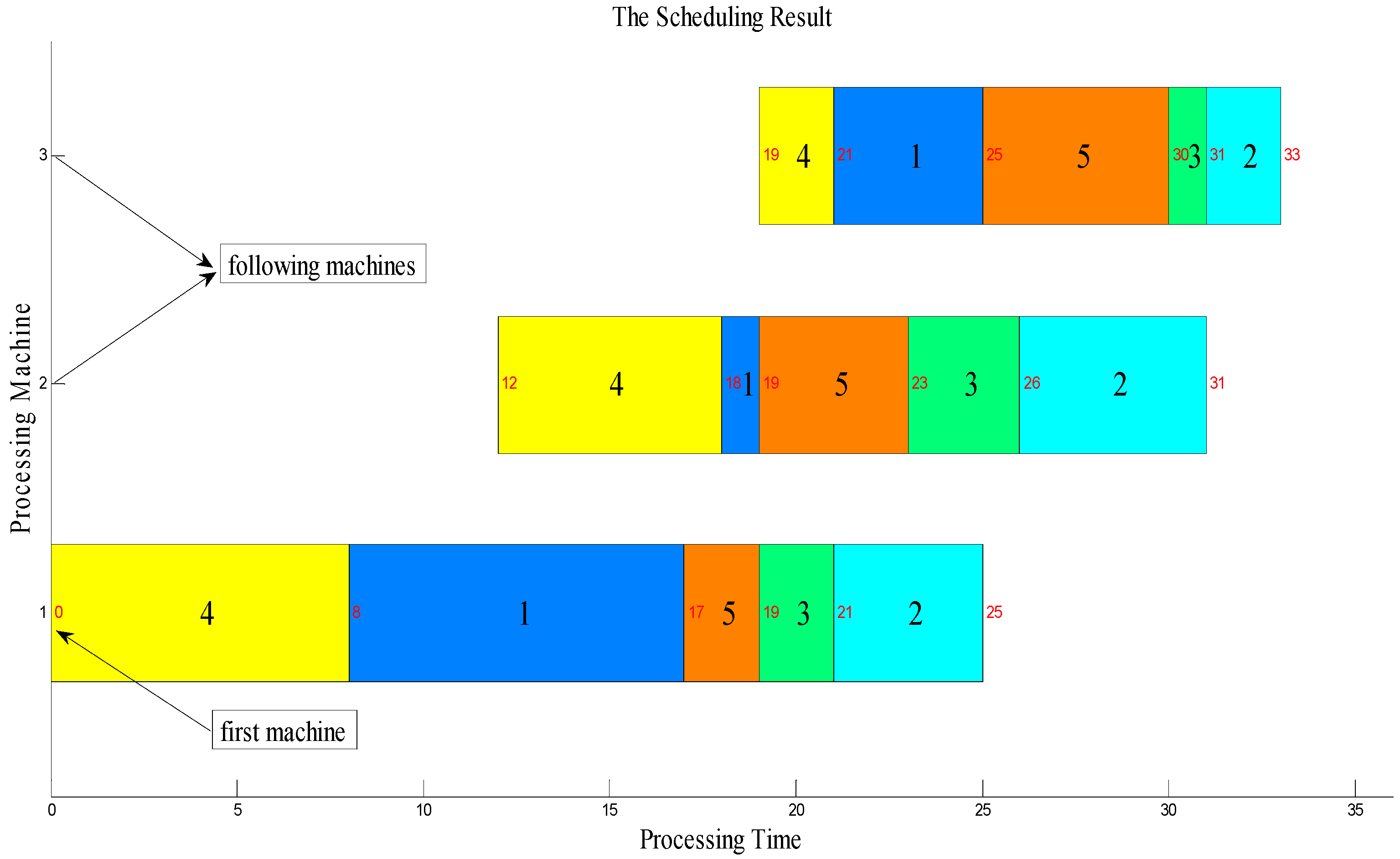
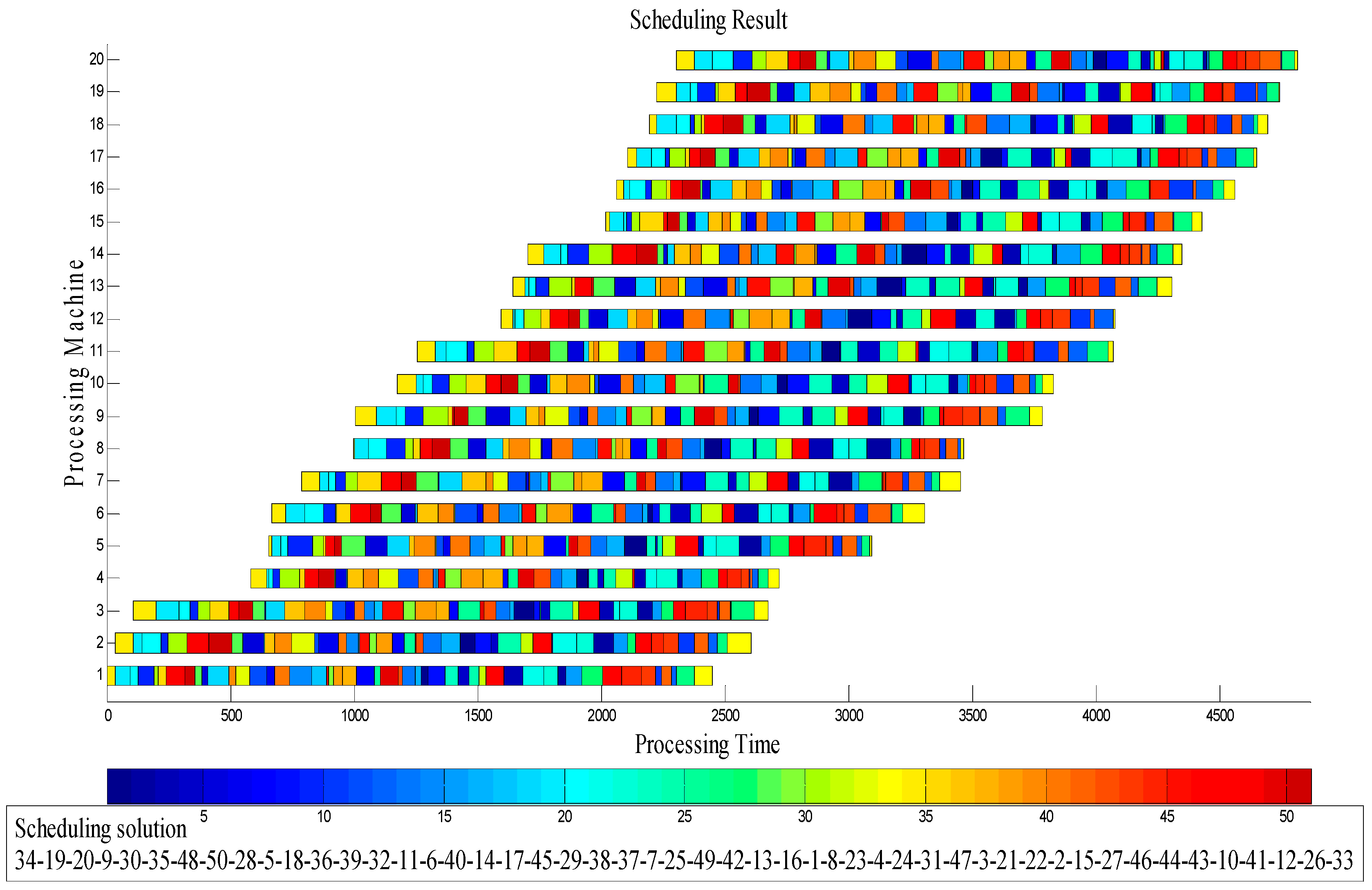
3.1. Solution Representation

All of the solutions in the traditional estimation of distribution algorithms (EDAs) are designed for continuous optimization problems. As a typical discrete optimization problem, the NIPFSP has distinctive features in its solutions. Thus, a discrete vector decoding method is employed as the solution representation. In particular, each discrete vector demonstrates a solution for the NIPFSP. For example, the discrete vector π = {6, 4, 5, 1, 3, 2} is a scheduling solution of jobs processed in the order of 6, 4, 5, 1, 3, and 2 for the NIPFSP. Each decoded solution in this decoding method shows the unique scheduling result for the NIPFSP. A hybrid discrete algorithm can also be designed to solve the NIPFSP with more efficiency than continuous algorithms. Given that job i is represented by the element π(i), a solution can be decoded as a processing vector π as illustrated in Figure 3.

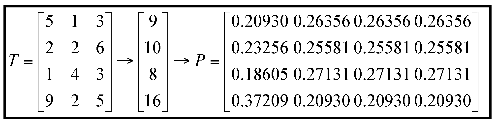
3.2. Initialization and Probability Model

Given that each individual is a solution representation as previously described, individuals are generated randomly in the initial population. The individuals in this method are randomly distributed in the entire solution space and have suitable diversity by uniform design. An individual is constructed by the NEH heuristic during the initialization to guarantee the initial population with a certain quality [11].
The probability model is the core brain of the EDA, which is commonly adopted to describe the distribution of the searching solution space. The probability matrix for describing the probability model is built based on several superior solution individuals during the iteration. New solution individuals are then obtained by sampling the probability matrix in the EDA. Therefore, improving the EDA performance is highly advantageous when the probability matrix contains the knowledge from the problems. This study focuses on the NIPFSP. The optimization objective is to determine the best scheduling solution with total tardiness minimization. Therefore, a modified probability matrix building method is proposed by taking advantage of the knowledge from the processing matrix T and designed solution representation. The designed probability matrix P is related to the job processing vector.
P = [ p 11 ( l ) p 12 ( l ) p 1 n ( l ) p 21 ( l ) p 22 ( l ) p 2 n ( l ) p n 1 ( l ) p n 2 ( l ) p n n ( l ) ]
Element pij(l) in the probability matrix P represents the probability that job j appears before or in the i-th position at the l-th iteration. The value of pij(l) refers to the importance of a job when decoding a solution into a schedule. As the processing matrix T can be calculated to obtain the total processing time of each job, the original probability matrix P is designed considering the knowledge of the longest total processing time job priority principle and roulette wheel selection. The original probability matrix P’s concrete implementation process is illustrated as follows:
T = [ T 11 T 12 T 1 m T 21 T 22 T 2 m T n 1 T n 2 T n m ] j = 1 m T 1 , j j = 1 m T 2 , j j = 1 m T n , j    P = [ p 11 ( 1 ) p 12 ( 1 ) p 1 n ( 1 ) p 21 ( 1 ) p 22 ( 1 ) p 2 n ( 1 ) p n 1 ( 1 ) p n 2 ( 1 ) p n n ( 1 ) ] p i , 1 ( 1 ) = j = 1 m T i , j i = 1 n j = 1 m T i , j     p i , j ( 1 ) = 1 p i , 1 n 1 ( 1 i n ; 2 j n ; i , j N + )
The sum of each row and column in the original probability matrix P is evidently one, which fits the requirement of the job processing vector for the sum of each row. The column element still represents the probability that job j appears before or in the i-th position at the first iteration. The amount of the row elements only contains the knowledge from the processing matrix T. An example for better illustrating the process of generating the original probability matrix P is shown in Figure 4.

3.3. Lévy Flight Strategy in CS

The CS algorithm was developed by Yang and Deb [23] and is a new population-based metaheuristic algorithm inspired by nature. The CS algorithm simulates the cuckoo process to determine a suitable nest location to build an optimization process. The cuckoos have a special ability to lay their eggs in another host’s nest, which was recently laid in by the host. The cuckoos lay their eggs among the eggs that were recently laid by the host, or even throw away the host’s eggs to increase the successful probability of their own eggs hatching. However, the host can find extraneous eggs and throw them away, or even rebuild a nest in other places. This scenario is a key process to encourage growth and prepare the body for reproduction. Several eggs are hatched successfully, and new individuals arrive at a new suitable nest location through Lévy flights [33]. Lévy flights are a global random walk; thus, this strategy provides the algorithm with the capability to search globally and locally. It then converges to the global optimality by exploring the search space efficiently even by the end of the iteration.
A discrete partially-mapped crossover (PMX) operation is introduced in the CS as a novel approach to conceal the cuckoo’s eggs and constitute a well-behaved hybrid algorithm. PMX can be viewed as an extension of a two-point crossover. It is an efficient mechanism to mix the partially optimal information of an individual to obtain a better job processing vector. The hybrid algorithm then becomes suitable for the discrete NIPFSP. Nevertheless, another procedure can legalize the new individuals, which are caused by the simple two-point crossover. The node repetition in the PMX crossover can be avoided by utilizing a mapping function. Therefore, the PMX searches for many new better individuals without increasing the computational complexity. The entire procedure is shown in Figure 5.

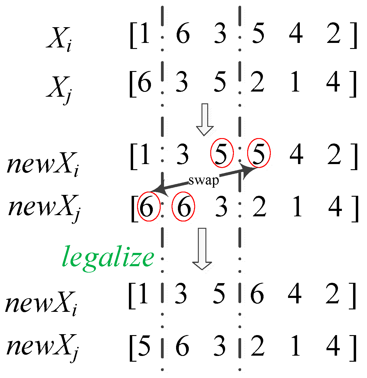
3.4. Updating Mechanism

Each optimization algorithm implements the population optimization through the iterative approach for solving the problem. Individuals with high fitness can provide search directions to attain the optimum solution in the NIPFSP. Thus, we obtain several better individuals in the population after a series of operations. We can then utilize the information in these individuals to update the probability model P. The details to update the probability model P are described in Equations (5) and (6). The probability model is directed toward the space that contains better solutions based on the top 10% of the best individuals. The search procedure must also track the potential searching region.
p i j ( l + 1 ) = ( 1 α ) p i j ( l ) + α S P × i a = 1 S P I i j a ;
I i j = { 1 ,   if   job   j   appears   before   or   in   position   i 0 ,   else ,
where α ( 0 , 1 ) is the learning rate from the new better individuals, and Ii,j describes whether job j is located before position i. Considering the operation of the SP better individuals in Section 3.5, the value of α can be set to be slightly large. A sufficient strategy can maintain the exploration in the HEDA_CS in the aforementioned operation. As an operation to obtain better knowledge information in relatively better solutions, the α value must be set as extremely small. This scenario is also an updating mechanism to obtain new individuals during the iteration.

3.5. Knowledge-Based Local Search

A knowledge-based local search is designed as an operator during the iteration to improve the exploitation capability of HEDA_CS. A critical path for the PFSPs refers to a continuous job-path from the beginning to the end of the solution with no idle condition between any two jobs [34]. Thus, this continuous job-path contains full processing knowledge of the NIPFSP with the total tardiness criterion minimization. Considering the variable neighborhood search [35], a suitable knowledge-based local search is designed in the HEDA_CS to solve the NIPFSP with the total tardiness criterion minimization. The insertion operator presents superior performance in the local search strategy. The knowledge-based local search mainly relies on such a partial subsequence insertion operator. In particular, the local search algorithm initially fetches a sequence from the job processing vector (i.e., an individual from SP better individuals). The length of the subsequence is at a maximum of n rounded down to the nearest whole unit. Several job numbers can then be obtained, which are the elements of the fetched sequence. Each fetched job is inserted to all of the possible positions of the remaining sequences. Only the best subsequence that has better fitness than the others is retained. Finally, a complete job sequence is obtained (i.e., an individual that has a minimal total tardiness criterion in such a job processing vector). If the final individual is different from the original individual, then the aforementioned iteration steps are repeated until the individual is consistent. The better solutions are updated with high exploration quality in this knowledge-based local search.

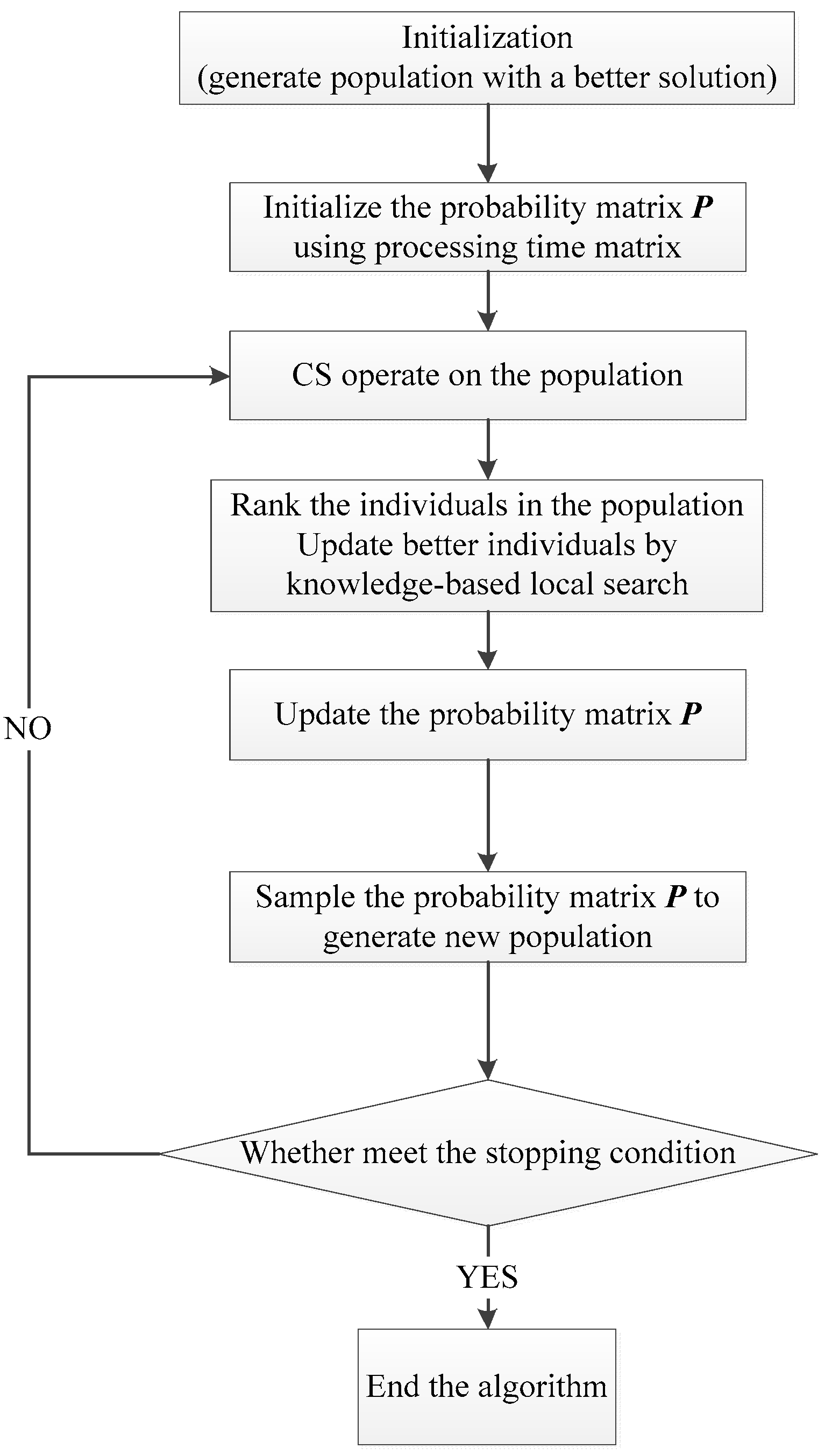
3.6. Overall Implementation

The flowchart of the HEDA_CS for solving the NIPFSP with the total tardiness criterion minimization is illustrated in Figure 6 with the aforementioned designed procedure. At the beginning of the hybrid algorithm, a population is generated with a better solution provided by the NEH heuristic. The probability matrix P is initialized by obtaining the knowledge of the processing time matrix T, and then a CS operator is implemented. Given that several individuals are optimized in the population, all of the individuals are ranked with high fitness (i.e., low total tardiness). The SP better ranked individuals enhance the exploitation by the knowledge-based local search. The probability matrix P is then updated on the basis of the job processing sequence information represented by these better individuals. A new population can be generated by sampling the probability matrix P based on the updating mechanism of the EDA. Given that the stopping condition is not met in the HEDA_CS, the algorithm is iterated to the max generation (Maxgeneration).
The computational complexity at the HEDA_CS iteration can be roughly analyzed as follows. The CS strategy in the updating process requires computational complexity of O(PopSize/2) by the PMX operator on the population. Computational complexity of O(SP × n2) is also observed. Each new generated individual in the sampling process is generated by the roulette strategy with computational complexity of O(n2). The aforementioned analysis shows that the computation complexity of the proposed HEDA_CS is not excessively large. It can solve the NIPFFSP with the total tardiness criterion minimization within an acceptable range of calculations.

4. Results and Analysis

Many tests are performed by utilizing the novel Ruiz benchmark instances in 2015 to investigate the performance of the proposed HEDA_CS [30]. All of the data can be obtained at http://soa.iti.es (accessed on 16 April 2017). These novel benchmark instances are near the real production process and have practical significance. Each Ruiz instance has the same structure with Taillards’ instances. Several case studies can be easily conducted utilizing the said algorithm. The due date of the i-th job is calculated as d i = λ · j = 1 m T i , j [36], where λ represents the tightness factor, T i , j is the processing time of i-th job processed on the j-th machine, and m is the total machine number. The tightness factor λ is set as 1, 2, and 3 to demonstrate the due date loose, medium, and tight, respectively. For the optimization objective of due date, the tightness factor can be seen as a different relaxation condition. Three values of the tightness factor λ represent three different requirements in the processing environment.
All of the experiment results are evaluated by average relative percentage deviation (ARPD) [37] to better evaluate the HEDA_CS performance. Thus,
ARPD = a v g G b e s t G b e s t × 100 ,
where Gbest is the total tardiness of the best solution obtained by all of the compared algorithms, and avg corresponds to the average value of the total tardiness of the solution obtained by a selected algorithm. So the lower value of the ARPD means that better solutions are achieved.
The proposed HEDA_CS is coded in C++ (Visual Studio 2012) and run on a PC with an Intel(R) Core(TM) i7-2600 CPU 3.40 GHz and 2.85 GB of available main RAM. The computation results demonstrate the quality of the proposed HEDA_CS. The hybrid strategy shows its suitable performance in solving NIPFSP. The following subsections describe the exhaustive concept of the parameter setting, computational results, and discussion.

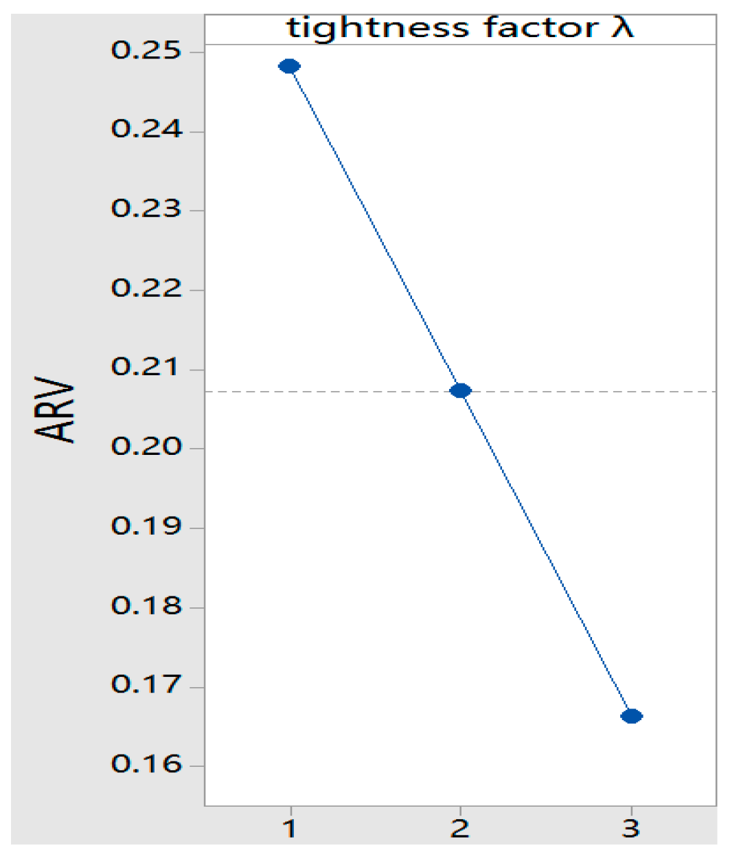
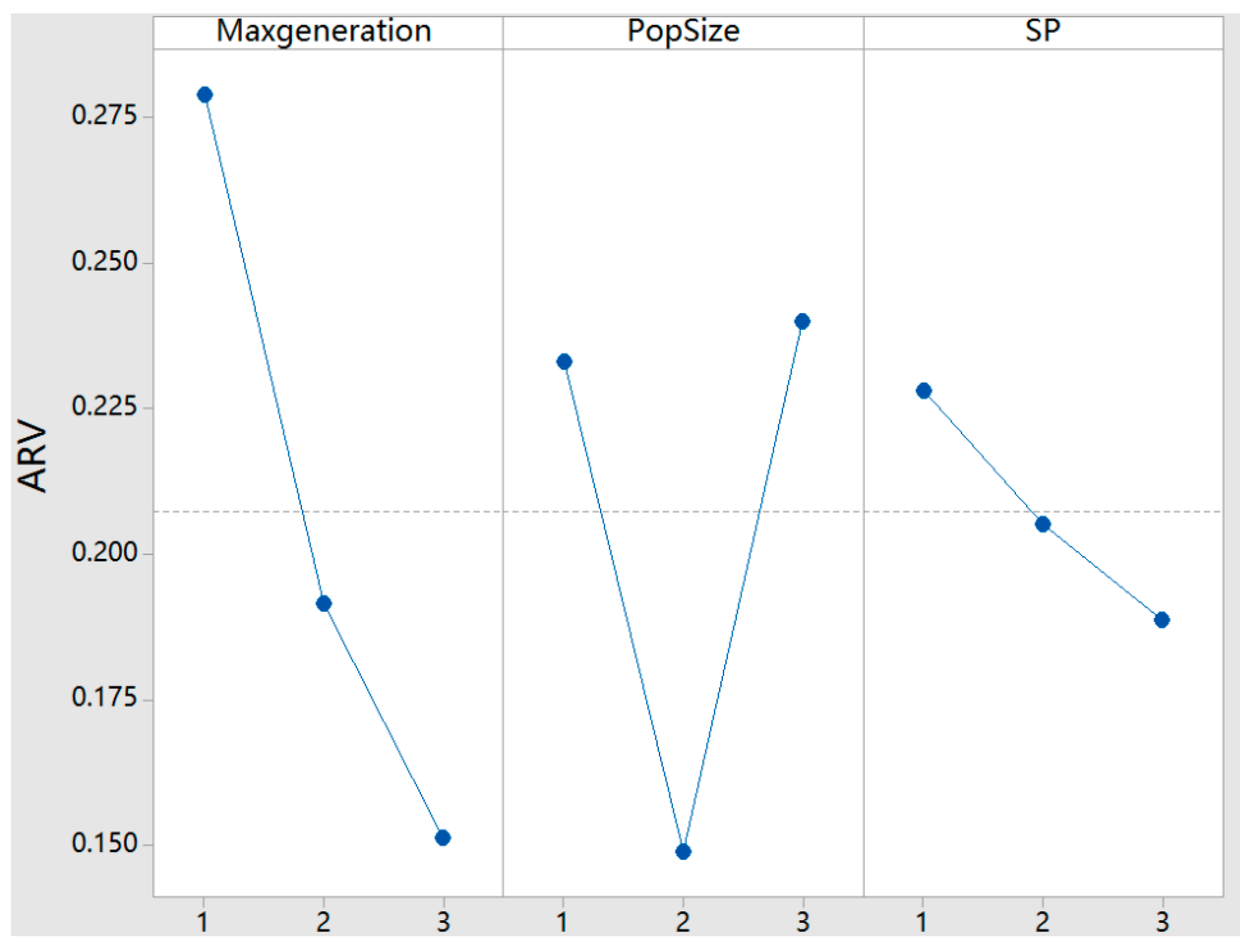
4.1. Parameter Setting

The three main parameters in the proposed HEDA_CS are as follows: Maxgeneration (iteration number), PopSize (population size), and SP (number of the superior ranked individuals in the population). All of the instances containing 60 jobs and 10 machines from the Ruiz benchmark instances are employed to adjust the said parameters. Another benchmark set is utilized to test the performance of the algorithm in the next section. An orthogonal experimental design method [38] is implemented to investigate the influence of these parameters on the HEDA_CS performance.
Given that the tightness factor λ has three different values to demonstrate the due date loose, medium, and tight, the three main parameters can be set differently under different tightness factors. The three levels of each main parameter are listed in Table 1. The HEDA_CS for each experiment environment run each instance 50 times independently (i.e., 50 × 10 × 9 = 4500 times). The entire orthogonal experiment is listed in Table 2. We can then obtain the trends of the tightness factor λ shown in Figure 7, which shows that the trends of the tightness factor λ is equal to its definition in different conditions. When the value of the tightness factor λ is large, the NIPFSP with the total tardiness criterion can be easily solved. Calculating the results in the orthogonal experiments yields the range and rank of the main parameters in the HEDA_CS as listed in Table 3. The trends of the main parameters in the HEDA_CS are shown in Figure 8. Maxgeneration has the most significant impact in the HEDA_CS, which is followed by PopSize. Given the experiment results, the recommended settings for the main parameters in the HEDA_CS are as follows: Maxgeneration = 1000, PopSize = 50, SP = 10. Such parameter settings can improve the efficiency of the HEDA_CS.

4.2. Results and Comparison of the Instances

Six sets of benchmark instances are selected from the Ruiz benchmark instances and are used to test the performance of the proposed HEDA_CS. Each set contains 10 different benchmarks with the same job and machine numbers. The factors and levels of these benchmarks are listed in Table 4. The benchmarks can generally describe the NIPFSP characteristics with the total tardiness criterion minimization. The range of the processing time distribution is U(1, 100). The selected benchmark job is in the range of [40, 50, 60, 100]. The number of process machines is in the range of [20, 40, 60].
The proposed HEDA_CS is compared with several existing algorithms, such as GA, IEDA, and CS, by utilizing these instances. For each instance, all of the algorithms are run 20 times each. The computational results are summarized in Table 5, Table 6 and Table 7 with different values of the tightness factor λ. The HEDA_CS obtained nearly all of the total tardiness minimization of the instances. The convergence curves of the four algorithms that solved the instance VFR100_20_3_Gap are shown in Figure 9. The best Gantt charts obtained by the HEDA_CS for better illustrating the scheduling production process and providing the actual production reference for engineers are shown in Figure 10 and Figure 11. Figure 10 illustrates the best scheduling solution of the instance VFR40_20_1_Gap under tight factor λ = 1. After enough iterations, the scheduling solution [36-7-17-6-20-5-29-1-13-26-19-38-28-24-9-25-3-31-30-14-4-21-2-35-11-34-15-8-32-37-10-39-12-27-18-33-40-16-22-23] is obtained by the proposed HEDA_CS. Following this scheduling solution, the 40 jobs in the instance VFR40_20_1_Gap can be processed with the lowest total tardiness among all of the solutions achieved during the iteration in HEDA_CS. Figure 11 illustrates the best scheduling solution of the instance VFR50_20_6_Gap under the tight factor λ = 2. This instance contains 50 jobs. Its best scheduling solution is [34-19-20-9-30-35-48-50-28-5-18-36-39-32-11-6-40-14-17-45-29-38-37-7 -25-49-42-13-16-1-8-23-4-24-31-47-3-21-22-2-15-27-46-44-43-10-41-12-26-33], which has lower total tardiness than the other solutions. To enhance the expression optimal scheduling result in the Gantt chart, each job has a unique color. The tight connection between neighbouring jobs reflects the no idle tight constraint.

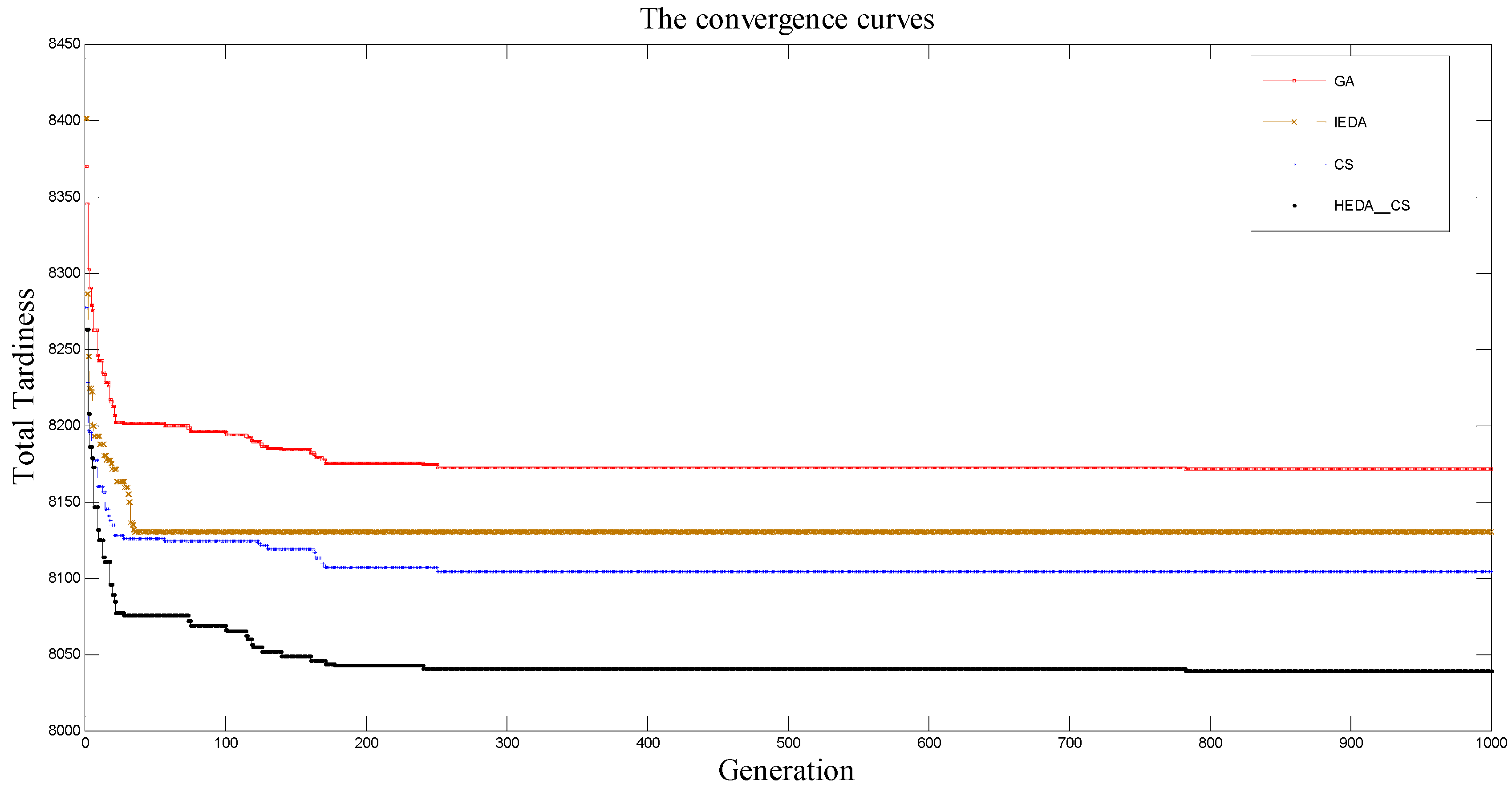
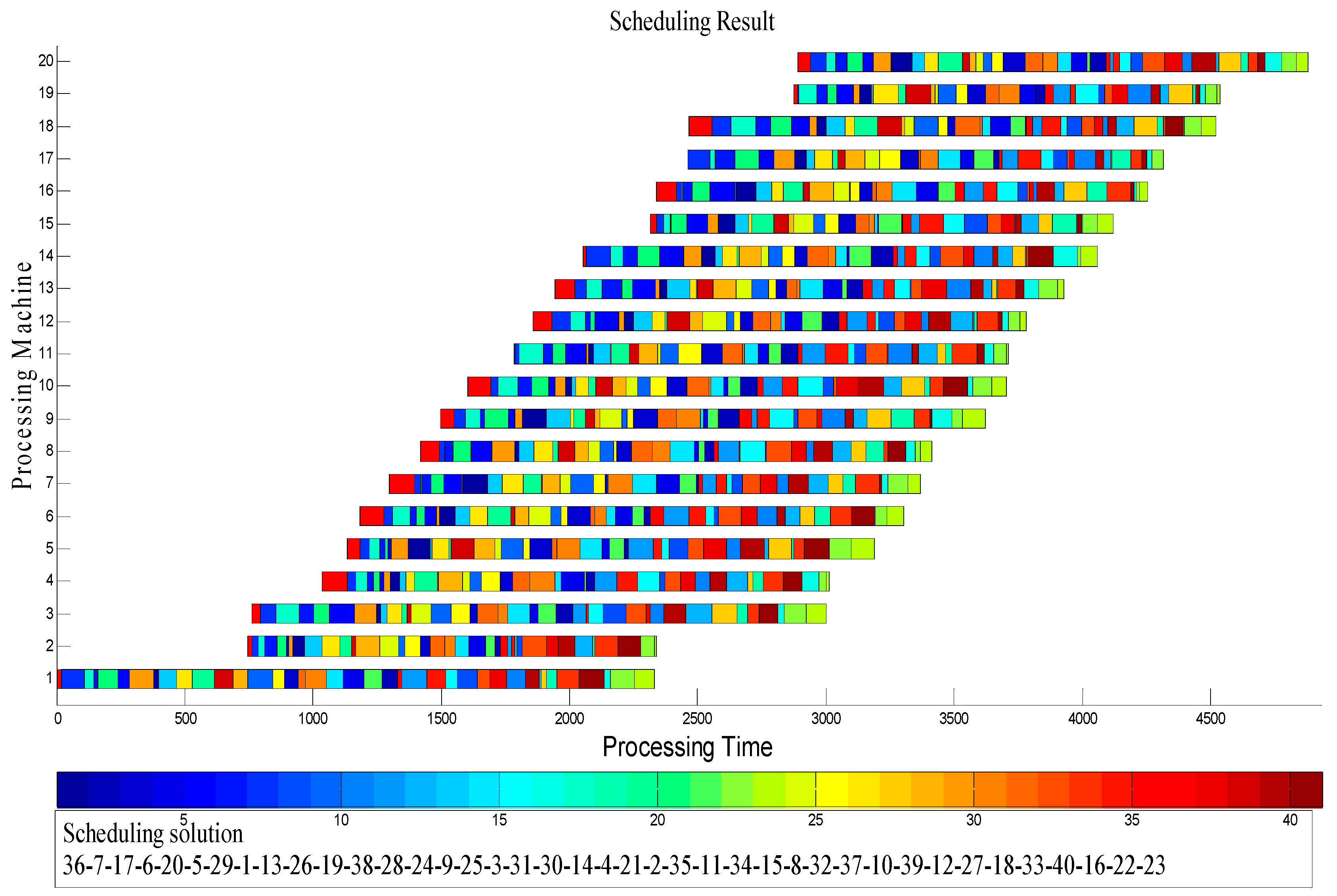
4.3. Discussion of Experimental Results

The performance of the proposed HEDA_CS is tested and compared with several existing algorithms by calculating the group of instances in the aforementioned sections. The comparative results show that the HEDA_CS performs better in solving the benchmark instances than the other algorithms. Table 5, Table 6 and Table 7, show that the proposed HEDA_CS obtains nearly the best scheduling solution with better total tardiness than the compared algorithms at all tightness factor scenarios. The convergence curves show that the proposed HEDA_CS is more efficient than the other algorithms. The proposed HEDA_CS can still continue to optimize the total tardiness of the NIPFSP after much iteration. The discrete job vector coding method can help optimize the HEDA_CS operator. Hence, this hybrid strategy can better balance the HEDA_CS exploration and exploitation. The Gantt chart arrangement is regular. The optimization results can also improve the production process effectively.

5. Conclusions and Future Work

This study proposes an effective and efficient HEDA_CS to solve the NIPFSP with the total tardiness minimization. A time point-based problem formulation is demonstrated with an example. As a novel hybrid discrete algorithm, a discrete vector decoding method is utilized in the HEDA_CS. Several operators are designed in the EDA with the knowledge of the process time matrix. The Lévy flight strategy enhances the EDA exploration. The PMX operator is applied in the CS, and the knowledge-based local search ensures the HEDA_CS exploitation. The HEDA_CS effectiveness is shown by utilizing the novel Ruiz benchmark instances and comparing with other algorithms. The HEDA_CS is highly efficient in solving the NIPFSP with the total tardiness minimization by setting the suitable main parameters. The proposed HEDA_CS performs best by comparing with other algorithm in solving the NIPFSP.
Future research can be devoted to other hybrid algorithm strategies. The new strategies which better combine the key characteristics of the problem will be more effective. In addition, the proposed approaches can be considered to extend to other scheduling problems with different objectives, such as total completion time, earliness, and makespan. Further studies can also focus on solving this problem with multi-objectives, since existing research mainly considered the single-criterion problems.

Acknowledgments

This work is supported by the National Natural Science Foundation of China (Grant No. 61573144, 61174040, 61673175) and the Fundamental Research Funds for the Central Universities under Grant 222201717006.

Author Contributions

The author Zewen Sun designed the algorithms and the experiments, analyzed the data, and wrote most of the manuscript. Xingsheng Gu discussed the original idea and the concept, gave many constructive comments, and was in charge of the paper.

Conflicts of Interest

The authors declare no conflict of interest.

References

  1. Cepek, O.; Okada, M.; Vlach, M. Note: On the two-machine no-idle flowshop problem. Nav. Res. Log. 2000, 47, 353–358. [Google Scholar] [CrossRef]
  2. Ruiz, R.; Maroto, C. A comprehensive review and evaluation of permutation flowshop heuristics. Eur. J. Oper. Res. 2005, 165, 479–494. [Google Scholar] [CrossRef]
  3. Adiri, I.; Pohoryles, D. Flowshop/no-idle or no-wait scheduling to minimize the sum of completion times. Nav. Res. Log. Q. 1982, 29, 495–504. [Google Scholar] [CrossRef]
  4. Woollam, C.R. Flowshop with no idle machine time allowed. Comput. Ind. Eng. 1986, 10, 69–76. [Google Scholar] [CrossRef]
  5. Saadani, N.E.; Guinet, A.; Moalla, M. Three stage no-idle flow-shops. Comput. Ind. Eng. 2003, 44, 425–434. [Google Scholar] [CrossRef]
  6. Bozorgirad, M.A.; Logendran, R. A comparison of local search algorithms with population-based algorithms in hybrid flow shop scheduling problems with realistic characteristics. Int. J. Adv. Manuf. Technol. 2015, 83, 1135–1151. [Google Scholar] [CrossRef]
  7. Ramezani, P.; Rabiee, M.; Jolai, F. No-wait flexible flowshop with uniform parallel machines and sequence-dependent setup time: A hybrid meta-heuristic approach. J. Intell. Manuf. 2013, 26, 731–744. [Google Scholar] [CrossRef]
  8. Samarghandi, H. Studying the effect of server side-constraints on the makespan of the no-wait flow-shop problem with sequence-dependent set-up times. Int. J. Prod. Res. 2014, 53, 2652–2673. [Google Scholar] [CrossRef]
  9. Vasile, M.-A.; Pop, F.; Tutueanu, R.-I.; Cristea, V.; Kołodziej, J. Resource-aware hybrid scheduling algorithm in heterogeneous distributed computing. Future Gener. Comput. Syst. 2015, 51, 61–71. [Google Scholar] [CrossRef]
  10. Zhu, X.; Li, X. Iterative search method for total flowtime minimization no-wait flowshop problem. Int. J. Mach. Learn Cybern. 2014, 6, 747–761. [Google Scholar] [CrossRef]
  11. Dong, X.; Huang, H.; Chen, P. An improved neh-based heuristic for the permutation flowshop problem. Comput. Oper. Res. 2008, 35, 3962–3968. [Google Scholar] [CrossRef]
  12. Baraz, D.; Mosheiov, G. A note on a greedy heuristic for flow-shop makespan minimization with no machine idle-time. Eur. J. Oper. Res. 2008, 184, 810–813. [Google Scholar] [CrossRef]
  13. Kalczynski, P.J.; Kamburowski, J. A heuristic for minimizing the makespan in no-idle permutation flow shops. Comput. Ind. Eng. 2005, 49, 146–154. [Google Scholar] [CrossRef]
  14. Pan, Q.K.; Wang, L. A novel differential evolution algorithm for no-idle permutation flow-shop scheduling problems. Eur. J. Ind. Eng. 2008, 2, 279–297. [Google Scholar] [CrossRef]
  15. Pan, Q.-K.; Tasgetiren, M.F.; Liang, Y.-C. A discrete differential evolution algorithm for the permutation flowshop scheduling problem. Comput. Ind. Eng. 2008, 55, 795–816. [Google Scholar] [CrossRef]
  16. Tasgetiren, M.F.; Pan, Q.-K.; Liang, Y.-C. A discrete differential evolution algorithm for the single machine total weighted tardiness problem with sequence dependent setup times. Comput. Oper. Res. 2009, 36, 1900–1915. [Google Scholar] [CrossRef]
  17. He, Q.; Wang, L. A hybrid particle swarm optimization with a feasibility-based rule for constrained optimization. Appl. Math. Comput. 2007, 186, 1407–1422. [Google Scholar] [CrossRef]
  18. Li, B.B.; Wang, L. A hybrid quantum-inspired genetic algorithm for multiobjective flow shop scheduling. IEEE Trans. Syst. Man Cybern. Part B Cybern. 2007, 37, 576–591. [Google Scholar] [CrossRef]
  19. Deng, G.; Gu, X. A hybrid discrete differential evolution algorithm for the no-idle permutation flow shop scheduling problem with makespan criterion. Comput. Oper. Res. 2012, 39, 2152–2160. [Google Scholar] [CrossRef]
  20. Tasgetiren, M.F.; Pan, Q.-K.; Suganthan, P.N.; Jin Chua, T. A differential evolution algorithm for the no-idle flowshop scheduling problem with total tardiness criterion. Int. J. Prod. Res. 2011, 49, 5033–5050. [Google Scholar] [CrossRef]
  21. Tasgetiren, M.F.; Pan, Q.-K.; Suganthan, P.N.; Buyukdagli, O. A variable iterated greedy algorithm with differential evolution for the no-idle permutation flowshop scheduling problem. Comput. Oper. Res. 2013, 40, 1729–1743. [Google Scholar] [CrossRef]
  22. Pan, Q.-K.; Ruiz, R. An effective iterated greedy algorithm for the mixed no-idle permutation flowshop scheduling problem. Omega 2014, 44, 41–50. [Google Scholar] [CrossRef]
  23. Yang, X.-S.; Deb, S. Cuckoo search via levy flights. In Proceedings of the 2009 World Congress on Nature & Biologically Inspired Computing (NaBIC 2009), Coimbatore, India, 9–11 December 2009; pp. 210–214. [Google Scholar] [CrossRef]
  24. Dubey, H.M.; Pandit, M.; Panigrahi, B.K. Cuckoo search algorithm for short term hydrothermal scheduling. In Power Electronics and Renewable Energy Systems: Proceedings of Icperes 2014; Kamalakannan, C., Suresh, L.P., Dash, S.S., Panigrahi, B.K., Eds.; Springer: New Delhi, India, 2015; pp. 573–589. [Google Scholar]
  25. Lim, W.C.E.; Kanagaraj, G.; Ponnambalam, S.G. A hybrid cuckoo search-genetic algorithm for hole-making sequence optimization. J. Intell. Manuf. 2014, 27, 417–429. [Google Scholar] [CrossRef]
  26. Majumder, A.; Laha, D. A new cuckoo search algorithm for 2-machine robotic cell scheduling problem with sequence-dependent setup times. Swarm Evolut. Comput. 2016, 28, 131–143. [Google Scholar] [CrossRef]
  27. Marichelvam, M.K.; Prabaharan, T.; Yang, X.S. Improved cuckoo search algorithm for hybrid flow shop scheduling problems to minimize makespan. Appl. Soft Comput. 2014, 19, 93–101. [Google Scholar] [CrossRef]
  28. Dasgupta, P.; Das, S. A discrete inter-species cuckoo search for flowshop scheduling problems. Comput. Oper. Res. 2015, 60, 111–120. [Google Scholar] [CrossRef]
  29. Niknam, T.; Azizipanah-Abarghooee, R.; Aghaei, J. A new modified teaching-learning algorithm for reserve constrained dynamic economic dispatch. IEEE Trans. Power Syst. 2013, 28, 749–763. [Google Scholar] [CrossRef]
  30. Vallada, E.; Ruiz, R.; Framinan, J.M. New hard benchmark for flowshop scheduling problems minimising makespan. Eur. J. Oper. Res. 2015, 240, 666–677. [Google Scholar] [CrossRef]
  31. Xu, Y.; Wang, L.; Wang, S.-Y.; Liu, M. An effective teaching–learning-based optimization algorithm for the flexible job-shop scheduling problem with fuzzy processing time. Neurocomputing 2015, 148, 260–268. [Google Scholar] [CrossRef]
  32. Wang, L.; Wang, S.; Xu, Y.; Zhou, G.; Liu, M. A bi-population based estimation of distribution algorithm for the flexible job-shop scheduling problem. Comput. Ind. Eng. 2012, 62, 917–926. [Google Scholar] [CrossRef]
  33. Viswanathan, G.M.; Afanasyev, V.; Buldyrev, S.V.; Murphy, E.J.; Prince, P.A.; Stanley, H.E. Levy flight search patterns of wandering albatrosses. Nature (London) 1996, 381, 413–415. [Google Scholar] [CrossRef]
  34. Grabowski, J.; Wodecki, M. A very fast tabu search algorithm for the permutation flow shop problem with makespan criterion. Comput. Oper. Res. 2004, 31, 1891–1909. [Google Scholar] [CrossRef]
  35. Dong, X.; Nowak, M.; Chen, P.; Lin, Y. Self-adaptive perturbation and multi-neighborhood search for iterated local search on the permutation flow shop problem. Comput. Ind. Eng. 2015, 87, 176–185. [Google Scholar] [CrossRef]
  36. Tasgetiren, M.F.; Pan, Q.-K.; Suganthan, P.N.; Oner, A. A discrete artificial bee colony algorithm for the no-idle permutation flowshop scheduling problem with the total tardiness criterion. Appl. Math. Model. 2013, 37, 6758–6779. [Google Scholar] [CrossRef]
  37. Wang, S.-Y.; Wang, L. An estimation of distribution algorithm-based memetic algorithm for the distributed assembly permutation flow-shop scheduling problem. IEEE. Trans. Syst. Man Cybern. Syst. 2016, 46, 139–149. [Google Scholar] [CrossRef]
  38. Masselink, G.; Ruju, A.; Conley, D.; Turner, I.; Ruessink, G.; Matias, A.; Thompson, C.; Castelle, B.; Puleo, J.; Citerone, V.; et al. Large-scale barrier dynamics experiment II (bardex II): Experimental design, instrumentation, test program, and data set. Coast. Eng. 2016, 113, 3–18. [Google Scholar] [CrossRef]
Figure 1. Permutation flow shop scheduling problem (PFSP) illustration.
Sustainability 09 00953 g001
Figure 2. Example of a no idle PFSP (NIPFSP) problem with five jobs and three machines.
Sustainability 09 00953 g002
Figure 3. Solution representation in HEDA_CS.
Sustainability 09 00953 g003
Figure 4. Example of generating the original probability matrix P.
Sustainability 09 00953 g004
Figure 5. Demonstration process example of a PMX crossover in HEDA_CS.
Sustainability 09 00953 g005
Figure 6. Flowchart of the HEDA_CS for NIPFSP with the total tardiness criterion minimization.
Sustainability 09 00953 g006
Figure 7. Factor trends of the tightness factor λ in NIPFSP with the total tardiness criterion minimization.
Sustainability 09 00953 g007
Figure 8. Factor trends of main parameters in the HEDA_CS.
Sustainability 09 00953 g008
Figure 9. Convergence curves of the instance VFR100_20_3_Gap (n = 100, m = 20, λ = 1).
Sustainability 09 00953 g009
Figure 10. Gantt chart of the instance VFR40_20_1_Gap (n = 40, m = 20, λ = 1) obtained by HEDA_CS.
Sustainability 09 00953 g010
Figure 11. Gantt chart of the instance VFR50_20_6_Gap (n = 50, m = 20, λ = 2) obtained by HEDA_CS.
Sustainability 09 00953 g011
Table 1. Factor levels of the three main parameters.
Tightness Factor λ Main ParametersFactor Levels
1, 2, 3Maxgeneration100(1), 500(2), 1000(3)
1, 2, 3PopSize10(1), 50(2), 100(3)
1, 2, 3SP5(1), 8(2), 10(3)
Table 2. Orthogonal experiments array.
Experiment NumberTightness Factor λ Main ParametersARV
MaxgenerationPopSizeSP
11100(1)10(1)5(1)0.3664
21500(2)50(2)8(2)0.1719
31100(1)100(3)10(3)0.2064
42100(1)50(2)10(3)0.2021
52500(2)100(3)5(1)0.2449
621000(3)10(1)8(2)0.1749
73100(1)100(3)8(2)0.2686
83500(2)10(1)10(3)0.1571
931000(3)50(2)5(1)0.0728
Table 3. Average value of the ARPD in different main parameter factor levels.
Factor LevelMain Parameters
MaxgenerationPopSizeSP
10.27900.23300.2280
20.19150.14890.2051
30.15140.24000.1887
Range0.12770.09100.0393
Rank123
Table 4. Factors and their levels for the selected Ruiz benchmarks.
FactorsLevels
Number of jobs40, 50, 60, 100
Number of machines20, 40, 60
Processing time on each machineU(1, 100)
Table 5. Comparison results on each set of benchmark problems ( λ = 1).
ProblemGAIEDACSHEDA_CS
AVEMINMAXAVEMINMAXAVEMINMAXAVEMINMAX
n = 40, m = 201.130.331.980.860.031.890.850.091.790.830.001.82
n = 50, m = 201.310.452.050.940.231.870.890.101.770.770.001.70
n = 60, m = 201.931.034.261.310.353.061.380.212.890.730.001.52
n = 100, m = 202.361.315.181.530.363.861.210.183.410.430.000.93
n = 100, m = 402.532.136.311.430.614.191.100.531.950.850.001.76
n = 100, m = 603.763.357.511.511.034.511.430.992.970.940.001.92
Average2.171.434.551.260.443.231.140.352.460.760.001.61
Table 6. Comparison results on each set of benchmark problems ( λ = 2).
ProblemGAIEDACSHEDA_CS
AVEMINMAXAVEMINMAXAVEMINMAXAVEMINMAX
n = 40, m = 201.140.292.070.890.012.130.910.061.930.890.001.84
n = 50, m = 201.190.362.841.180.172.521.090.152.210.750.001.88
n = 60, m = 201.671.072.651.510.683.151.380.232.970.620.001.42
n = 100, m = 202.131.793.091.871.013.241.570.293.310.410.000.92
n =100, m = 402.311.934.352.010.974.131.510.353.150.930.001.99
n = 100, m = 602.602.014.321.971.135.011.890.513.681.160.002.07
Average1.841.243.221.570.663.361.390.272.880.790.001.69
Table 7. Comparison results on each set of benchmark problems ( λ = 3).
ProblemGAIEDACSHEDA_CS
AVEMINMAXAVEMINMAXAVEMINMAXAVEMINMAX
n =40, m = 200.830.132.110.790.091.990.810.051.810.780.001.93
n = 50, m = 200.990.272.250.860.142.070.820.011.830.780.001.62
n = 60, m = 201.461.122.690.970.312.210.950.162.120.670.001.52
n = 100, m = 201.681.532.861.310.462.561.160.252.510.420.000.93
n = 100, m = 401.791.672.901.460.512.731.310.292.751.020.001.85
n = 100, m = 602.141.892.981.580.592.641.620.362.811.280.002.12
Average1.481.102.631.160.352.371.110.192.030.830.001.66

