
Sustainable Optimization of Manufacturing Process Effectiveness in Furniture Production


1
Department of Business Economics, Technical University in Zvolen, T.G. Masaryka 24, 96053 Zvolen, Slovakia
2
Department of Management Theories, University of Žilina, Univerzitná 8215/1, 010 26 Žilina, Slovakia
*
Author to whom correspondence should be addressed.
Sustainability 2017, 9(6), 923; https://doi.org/10.3390/su9060923
Submission received: 31 March 2017
/
Revised: 12 May 2017
/
Accepted: 30 May 2017
/
Published: 1 June 2017
(This article belongs to the Special Issue Sustainability in Manufacturing)
Abstract
:Sustainable manufacturing is connected with the effectiveness of production processes. There are several solutions to improve manufacturing sustainability. This paper deals with the possibilities of the utilization of mathematical methods to solve optimization problems in the production process of furniture. The aim of the paper is to create a mathematical model of the key processes in order to maximize productivity and cost reduction by identifying key processes and parameters influencing manufacturing effectiveness. After identification of the parameters describing the key process (milling), an abstract model of the manufacturing process was created. Identified input parameters were the cutting velocity, feed rate, and a total volume of removed material. The output parameters were surface roughness, process duration, and process cost. The experimentally measured and calculated values of the output parameters were analyzed by a multiple regression tool. The method of an artificial neural network was used as a numeric method for optimization. The results showed that the maximal effectiveness of the sub-process can be achieved if the CNC machine is set at the cutting velocity of 4398.23 m·min−1 and feed rate of 11.00 m·min−1. Maximal values of the created neural network showed optimal values of input and output parameters.
1. Introduction
An improvement of business processes is necessary in order to maintain the competitiveness of the business and increase the financial performance. The enterprises have to carry out various innovative activities, not only for the outputs, but also for the processes. The presumption of effective management and a sustainable enterprise improvement are measuring, assessment, control, and further optimization of the enterprise processes. Efficiency and effectivity are the main parameters of processes optimization. These two terms relate to each other closely and are often confused, though there is a certain distinction in their definitions. While the effectiveness expresses the ability of completing the proper steps to achieve the purpose, in other words, the level which the system achieves in the relation to the level which was stated (the current output to the expected output), the efficiency describes the level when the system uses the proper sources in a proper way, so it addresses the question of whether we do the right steps in the right way (the currently used sources to anticipate source consumption) [1].
According to Leong et al. [2], there are five key dimensions of the effectiveness of a production process including costs, delivery efficiency, quality, flexibility, and innovation. Vickery, Dröbe, and Markland [3] synthesized the knowledge on priorities within the enterprise competitiveness raise. They included process flexibility: the ability to produce a few products so that the production remains cost efficient, i.e., it has the ability to rapidly adapt to changes in the product mix.
Hossain and Prybutok [4] designed the model of enterprise effectiveness management which consists of eight parts (innovation, competitive advantage, production output, customer-driven output, financial and market output, employee-driven output, process efficiency outputs, and leadership outputs). The process effectiveness measures included indicators of efficiency and effectiveness (cost savings, higher productivity, emission reduction, etc.), indicators of internal response ability (circle time, production flexibility, delivery time, adjustment time, etc.), specific indicators of office work/administration efficiency improvement and other support functions (innovation level, results of Six Sigma initiative, and so on), and indicators of supplier—customer relationships (reduction of supplier—customer chain management costs, reduction of supplies and input control, improvement of electronic data exchange, etc.).
In the manufacturing process, narrow spots occur. In a graphical concept, the narrow spot of the production is the narrowest spot in the line of manufacturing. It occurs at the moment when the work objects come to a certain point faster than the point is able to process. It can be said that it is a point of accumulation in the system. By optimizing, a manufacturing process is therefore needed to focus on the key or critical sub-process. The key sub-process is related to the manufacturing of the key product contributing to the final value of production at most. It could be used during the procedure of calculating individual product shares in the total sale of an analyzed company. The sub-process in which many errors occur provides a gap for improvement and optimization. The second important aspect is the interconnection of the sub-process to the entire production process and its efficiency, with an emphasis on the technological procedure. Therefore, higher weights are allocated to the procedural errors occurring in the first phases of the production process.
The second step by optimizing the task is to identify the essential parameters of the critical manufacturing sub-process (the process of chip formation in parts cutting). The variables which are necessary to be defined within the problem solution can be divided into three groups:
- Modern indicators of effectiveness, which are connected to the vision, strategy, and objectives of the reference enterprise, with an emphasis on critical success factors (CSF).
- Technical parameters of the sub-process to create a mathematical model that reflects the physical nature of the particular process.
- Technical and economic output parameters of the sub-process, reflecting its overall effectiveness, which is understood to be a complex goal consisting of cost minimization, quality maximization, and productivity.
Technical and economic output parameters are focused on the solution of an optimization problem. Optimization objectives are divided into the following three areas [5]:
- Input: optimization of raw materials, auxiliary materials, energy, human resources, investment, etc. (costs reduction);
- Output: optimization of products, by-products, emissions, cash recovery, etc. (quality improvement);
- In Side process: optimization of technical and economical indexes in terms of production efficiency, energy utilization, material yield, labor productivity, equipment operating rate, utilization of current funds, etc. (increasing of process productivity and flexibility).
Finding the optimal solution while maintaining the required product quality lies in the reduction of important factors of the manufacturing process which include material and energy consumption, costs related to the product development, and time. The change of the variables in the optimization problem design shall result in a reduction of material inputs, production costs, goods, material properties of the product, and at the end, in the minimization of the optimization task.
There exist several managerial methods and conceptions for process optimization. Analysis techniques applied during the optimization have to include all relevant data sources and the individual analysts have to be able to spot the right designs amongst a plethora of choices [6]. Nowadays, basic tools and methods of every manager include budgets and calculations, in addition to an effective and efficient usage of the Managerial Accounting information [7]. Zhou and Chen [8] developed a systematic optimized design methodology of the business process that also outlines the knowledge infrastructure of Business Process Reengineering (BPR) from strategic, tactical, and operational levels. Bencsik et al. [9] consider the Lean Management optimization method to be the most suitable for offering such solutions for changing the production environment, corresponding to productivity increase and cost reduction expectations. Howell [10] used the Taguchi approach to optimise the performance of the system in a minimum number of tests, without having to understand the mechanisms by which each parameter affected the system. Zhenov [11] and Simanova [12] consider the Lean and Six Sigma approaches to process optimization to be flexible because these methods allow their application by both manufacturing and service providing companies. Modern techniques, as well as Lean Six Sigma System, Lean Process Principles, Just-In-Time Production, and Total Quality Management, are focused on the responsible use of resources by eliminating waste [13,14].
The mathematical solution of the optimization problem requires an application of a suitable model with a finite number of parameters. These variables must be relevant considering the description of the most important characteristics of the problem being constructed [15].
According to Fusek and Halama [16], there are two principal methods of optimization tasks modeling, namely an analytical method and a numerical one. The analytical method provides the result achieved by mathematical analysis, including differential and integral calculations in the form of continuous functions. A numerical method is approximate. The problem of searching the continuous functions is altered to the problem of searching a finite number of unknown parameters due to which the searched functions approximate. This is referred to as discretization of a continuous model. The discretized model is solved via algebraic means, which have a limited number of steps. The numerical solution is principally available for any problem which is described mathematically. The most common method of a numerical solution approach is Artificial Neural Networks and the Finite Element Method.
Rubio et al. [17] described the general classification of optimization techniques and the main methodologies and tools employed for predicting the surface roughness. The techniques could be divided to Statistical Regression, Artificial Neural Networks, Fuzzy Set Theory, and Fuzzy Neural Networks from an empirical point of view. Furthermore, optimization tools and techniques are divided into two groups: a conventional one focusing on providing an Optimal Solution and Non-Conventional Techniques focusing on providing a Near Optimal Solution. Conventional Techniques include Design of Experiments (Taguchi Method, Factorial Design, and Response Surface Methodology) and Mathematical Iteractive Search (Dynamic Programming, Non-linear and Linear Programming). Non-Conventional Techniques include Meta-Heuristic Search (Genetic algorithm, Simulated Annealing, and Tabu Search) and Problem Specific Heuristic Search.
In the case of the automated recognition of space objects, the prediction of time sequence signals, and optimization problems, the use of the before mentioned methods seems rather useful and effective. These models are called Artificial Neural Networks—ANN. Formally, the network has the structure which is described by a directed graph with peaks (neurons) and directed edges (connections). One of the simplest types of networks is a multilayer network with feed-forward propagation, which has one input layer, one or more hidden layers, and one output layer. In general, the networks can be divided into two groups:
- Feed-forward networks—the signal is only propagated forward,
- Recurrent networks—some neurons present both input and output types.
In their paper, Xu and Lee [18] presented a novel milling process optimization method based on hybrid forward-reverse mappings (HFRM) of artificial neural networks. Mendyk et al. [19] used ANNs and genetic programming (GP) and developed a mathematical model of the drug dissolution (Q) from the solid lipid extrudes.
The continuous search for the optimization of processes presents one of the solutions for economic improvement and the sustainability of manufacturing process effectiveness. The aim of this article is to design a mathematical model for the optimization of the key sub-process effectiveness in furniture manufacturing, based on which it is possible to anticipate the levels of output parameters with different levels of input parameters. The model enables the sustainable process effectiveness in manufacturing at an optimal level.
2. Material and Methods
The first step in the optimization problem solution was to identify the critical sub-process of manufacturing, its specific parameters, procedure, and duration of individual steps in the due enterprise.
The key sub-process is the one which is associated with the manufacturing of the key product that contributes the most to the final value of the production. In the reference enterprise, we decided on the procedure of enumeration of the individual products share on the overall sale. The enterprise introduced 21 new products in 2014, which required substantial investment costs. The enterprise currently manufactures 48 products. Having consulted with a technologist in the enterprise, a wash basin closet was chosen as a reference item. The lead time (the time necessary to manufacture the product) was 34 min and 9.98 s. To optimize the process, it is necessary to concentrate on the activity with the biggest defect rate because it presents the space for improvement. The next important aspect is its link to the effectiveness of the overall manufacturing process, with an emphasis on the technological procedure. Considering this, it is important to correct the faults immediately and as early as in the initial stages of production so as not to incur costs in the further manufacturing of a faulty product. The critical sub-process in furniture manufacturing is the milling process.
The second step was to identify the essential parameters of the critical manufacturing sub-process (the process of chip formation in parts cutting-milling). The technical parameters of the sub-process (milling) describe its physical nature (spindle speed, cutting speed, feed rate, depth of cut, etc.). It is observed that the cutting speed is the most influential parameter for surface roughness, followed by the feed rate [20,21,22]. In addition, it was not possible to vary the depth of cut during the experiment in the reference enterprise. Therefore, the input parameters were the cutting speed and feed rate, which were varied. The depth of cut was constant (a = 1 mm) and a total volume of removed material was calculated. The output parameters of the process milling were the surface roughness, process duration, and process cost.
Having identified the parameters describing the manufacturing sub-process (cutting–milling), the next step was to create an abstract model of the manufacturing process which would allow an investigation of the manufacturing process using the mathematical description of the progression of the processes. The identified input parameters as independent variables were: the cutting speed (vc), feed rate (vf), and the total volume of removed material (V). By our experiment, the cutting speed and feed rate were varied using the CNC wood machine and in each variation, one output parameter (surface roughness) was experimentally measured and the other parameters were calculated. The variations of input variables used in the experiment are presented in Table 1.
To enumerate the total volume of the removed material, taking into account the complicated shape of the workpiece, we used the SketchAndCalc™ (Domains by Proxy, Scottsdale, AZ, USA) program, which was used to calculate the content of the removed area according to the cross-section of the workpiece in the blueprints. Other areas were deducted, and consequently, the value of the removed area was multiplied by the cumulated value of the length of the workpiece being machined. The volume of the removed material was calculated (V) according to following Equation:
where Sm is the size of the removed area, L is the length of the workpiece being machined, and POD is the number of workpieces being machined (cumulated sum).
Within the experiment, medium density fiberboard (MDF) was used. The fiberboards with a density of 750 kg·m−3 are manufactured from wood fibers, mainly spruce, which are bound by synthetic glue under the simultaneous effect of temperature and pressure. They meet the requirements of EN 622-1 and EN 622-5 standards. The thickness of the input material was 22 mm, the length 1000 mm, and width 630 mm. The material was milled under conditions stated in advance, while the thickness was the milling parameter and after the operation was finished, a sample of the dimensions: length 1000 mm, width 22 mm, and thickness 29 mm, was cut out. The particular sample was used for taking a sample object where the surface roughness was measured by two methods in the track of 11 mm (see Figure 1).
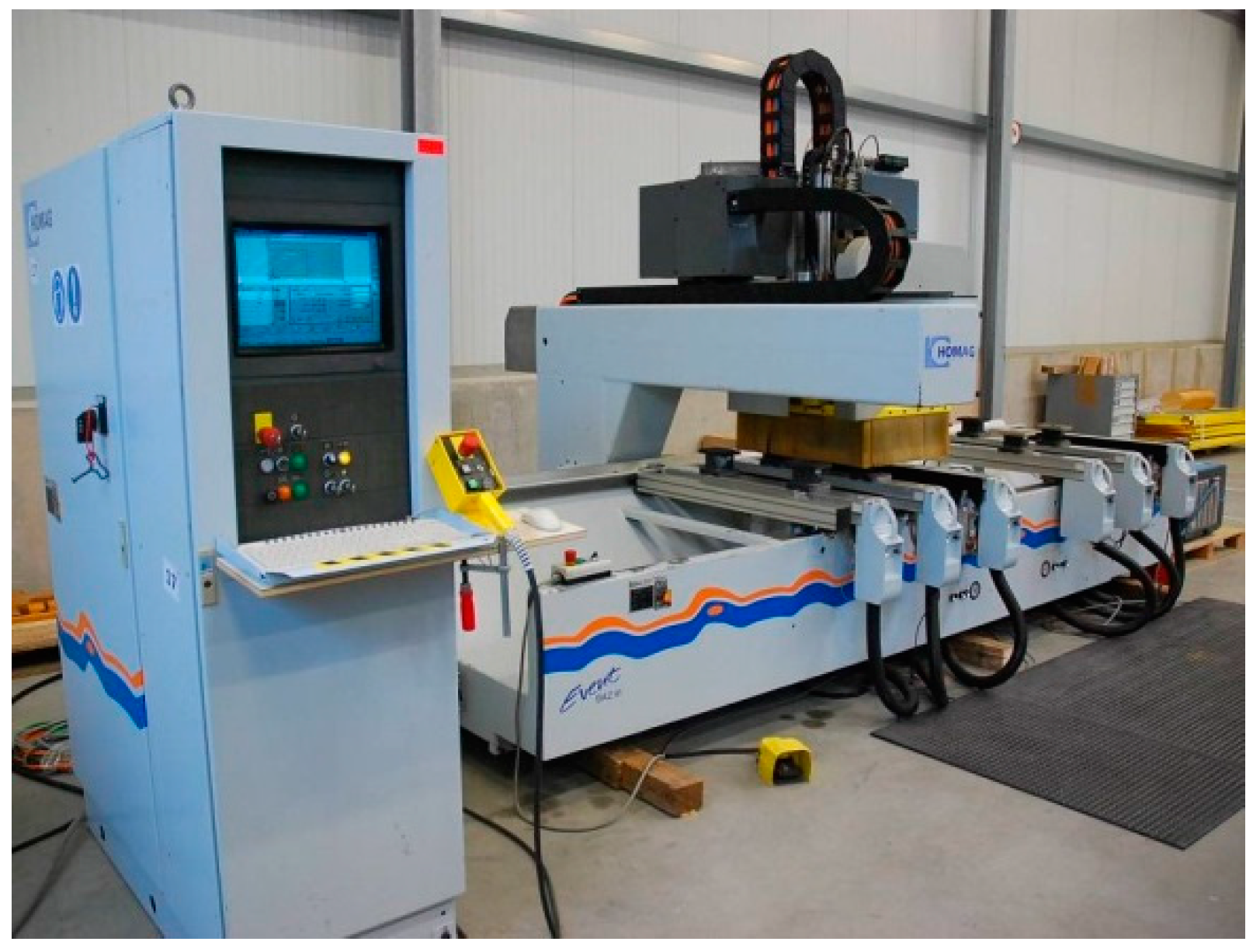
The samples were machined by a CNC wood machine of the HOMAG BOF 41/30/R make (see Figure 2). The overall performance of the machine is 21 kW and engine performance of the arbor is 7.5 kW, while the revolutions can be set in the range of 0 to 18,000 revolutions per minute. The operation span of the X axis is 3000 mm and the Y axis is 1150 mm. The dimensions of the operation table are 3400 mm × 1450 mm.
During the experiment, the arbor (Ø 100 mm) with three reversible milling blades made of hard alloy (T03SMG) was used.
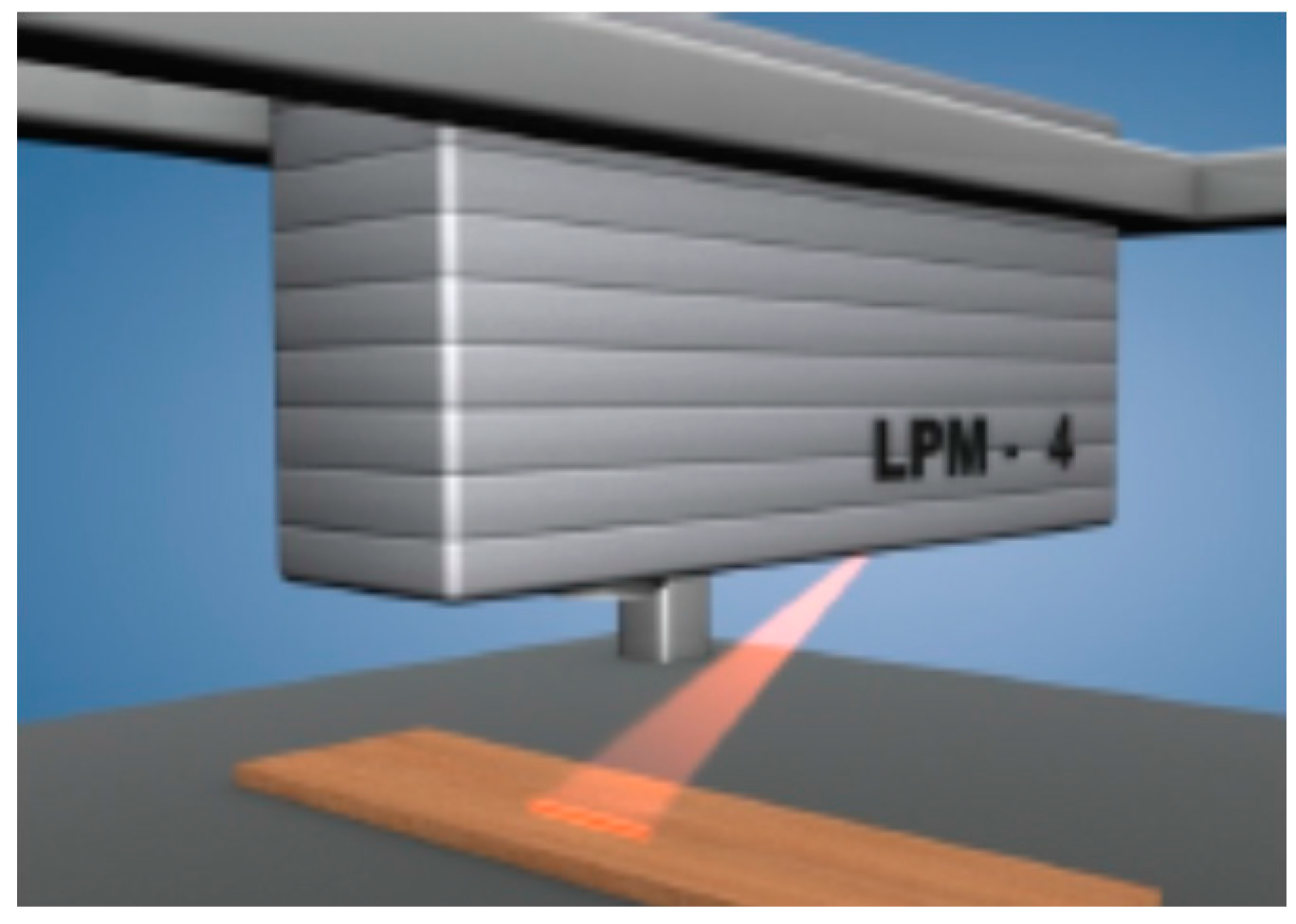
The first output parameter includes the quality indicator, surface roughness. The roughness parameter Ra was measured experimentally at the laser profile meter LPM 4 (see Figure 3), which was constructed at the Department of woodworking at the Technical University in Zvolen in cooperation with Kvant, s.r.o. (Kvant spol. s.r.o. Ltd, Bratislava, Slovakia). Siklienka et al. [23] characterized the machine as a compact laser profile meter serving to optically measure 2D profiles along a defined cut, in a contact-free manner on a triangulate basis. Then, the size of the Ra parameter was measured by a contact roughness tester MITUTOYO SJ-210 with a diamond stylus equipped with a support outrigger to be used in a manufacturing environment. The used detection methods were inductive and the range of the measurement was 350 µm (−200 µm to +150 µm). The length being measured was 12.5 mm. A testing sample was comprised of five measurements.
Consequently, the calculations of the output parameters of the critical sub-process were stated, comprising the process duration Ts and process costs NO.
The process duration was calculated according to the following Equation:
where Ts is the machine time, Tf is the milling time, and TFN is the idle time.
The total process costs (NO) were calculated as follows:
where NE represents the energy costs, NoP represents the labor costs (influenced by CNC setting), NUH is the cost of the arbor, and NFN represents the costs of the cutting blades.
The individual elements of the total costs were calculated by the Equations:
where V is the machine performance per hour in kW; TZ is the guarantee time of the arbor in min; TPaP is the time of failures and idle time for the machine in min; η is the efficiency; CE is the energy cost per kW hour; PPN is the percentage of the tool usage (25%); MH is the gross wage of a CNC operator—median; CUH is the price of the arbor; OZľ is the fund and tax payments 35.2%; TC is the total duration time of the sub-process; and NN is the cost non-affectable by the CNC setting.
In [24], the tool life cycle was calculated TL (10), and further, the percentage of removed life cycle was calculated considering the milling time. Additionally, the costs of the cutting blades made of hard alloy were calculated (11). The author [24] describes the calculation of constants CT (8) and m (9) in her experiment. The medium density fiberboard and solid carbide tool were used in the work, as well as in our experiment.
where CT is the constant, T is the tool duration, TL is the tool life, m is the exponent, vc is the cutting speed, Tf is the milling time, and CFN is the tool price.
The measured and calculated values were analyzed in the Statistica 12 program by a multiple regression tool. The following parameters were determined as independent variables: cutting speed vc, feed rate vf, and the total removed material volume V. The dependent variables were stated, respectively, as the surface roughness indicator Ra, machine time Ts, and the total influenceable costs of the process NO. Consequently, we used the numeric method of optimization of the machining processes, the method of the artificial neural network, which has rocketed in the last decades with the use of computer supported solutions. The main building unit of ANN is a perceptron, or the neuron model which receives the input signals through synaptic weights creating the weight vector . The output of the perceptron is given by the following relation [25]:
where f is the activation function of perceptron; net is the scalar product (dot product) of the scalar and input vectors; and θ is the the threshold of the neuron.
Data by the creation of an artificial neural network are divided into two samples: trained and tested. Through the data of the trained sample, a formula is created which describes the output parameters on the basis of the best input parameters. In the tested sample, the data are verified and the verification process is stopped when the deviation is at a minimal level.
The solution of the optimization problems by this method focused on the optimization of adjustment of the cutting velocity and speed rate of a CNC machine. The last step was to create relations of input parameters of the mathematical model and the overall effectiveness of the critical manufacturing sub-process through the abstraction method (selection of essential characteristics and so constructing a simplified model of only those characteristics or signs whose investigation can answer research questions of the scientific objectives of the paper) and defining the weights of the individual output parameters, taking into account the critical success factors of the referenced enterprise.
Considering the aim of the work, in particular creating a mathematical model of sub-process effectiveness optimization, the following hypothesis was stated and tested: There is a significant dependency between the identified input parameters and manufacturing process effectiveness represented by the cost level per sub-process, the quality of the workpiece being machined, and the total duration of the sub-process. The hypothesis verification was carried out via the multiple regression method and artificial neural network.
3. Results
In the furniture enterprise, the critical activity or sub-process of furniture manufacturing is the milling process because it has the most significant impact on the consequent activities. The cost value of sanding is directly proportional to the workpiece surface roughness degree after milling as the smooth surface with a minimum roughness is an important prerequisite to manage the surface finish. Aiming at the determination of the quality degree of the due sub-process, we measured the workpiece roughness by two methods described in the previous sections.
3.1. Measurement, Calculation of Parameters and Dependence Verification
The determined input and output parameters influencing the effectiveness of the milling process were measured and calculated within the experiment. Consequently, a dependence of the parameters was verified by the statistical multiply regression method.
In Table 2, the data relating to the measured values of the operation duration (Tf), the size of material removal per minute (MRR), the used energy amount for the particular operation (E) needed for the calculation of energy costs and calculated values of total material removal (V), the durability of the milling blade (TL), the median of the measured roughness Ra, and the overall costs of individual operations (NO) are illustrated. The presented values were measured and calculated by 18 variations of the cutting speed and feed rate (Nr.) mentioned in the previous section in Table 1.
The measured and calculated values were analyzed by the Statistica 12 program by multiple regression tools. There were stated as independent variables: cutting speed vc, feed rate vf, and total removed material volume V. The following parameters were selected in successive steps: surface roughness parameter Ra, machine time T, and overall controllable costs per operation NO.
The coefficient of correlation for the Ra variable is at the 0.70 level. Having calculated the determination coefficient (R2), which is 0.49, we can state that 49% of changes in the roughness can be explained as changes in the input variables. This coefficient is necessary to adjust and calculate the adjusted determination coefficient which contains correction for the number of explaining variables. In this case, it is (R2adj.) 0.38. As there is no big difference, we can state that the model did not include too many variables. The total value of test significance is lower than 0.02091, while the statistical significance level (α) was set at 0.05 so with 95% confidence, so it can be expressed that the Ra variable is statistically significantly dependent on the variables: cutting speed (vc), feed rate (vf), and total removed material (V). The standard error in the model estimate is 0.00109. All three input parameters (exogenous variables) are statistically significant because the value of significance is lower than 5% in all three cases. Coefficients b * for the individual variables express their relative influence on the dependent variable (see Table 3).
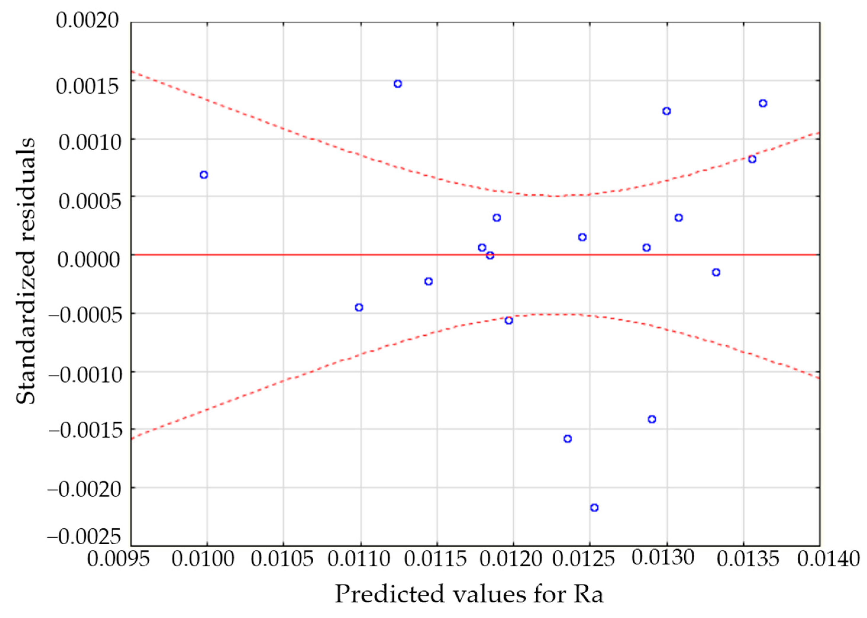
Model verification by model residual analysis was the next important step. The graph in Figure 4 is an illustration of the estimated values and residuals for the dependent variables Ra with a marked 95%-confidence interval.
As reported by the value distribution in the point graph, it can be claimed that model residuals are approximately distributed around the zero mean value, which means that the model is correctly specified. This statement was verified by a Shapiro-Wilkov test, with a significance value of p = 0.0915.
The test is not statistically significant because a zero hypothesis for the normality of residual distribution cannot be rejected. In other words, the residuals have a normal distribution, and therefore, the individual parameters of the regression line are correctly specified. The regression line is of the following form:
where Ra is the surface roughness, vc is the cutting speed, vf is the speed rate, V is the total material removal, and E is the energy consumption.
3.2. Estimation of Input Variables Impact on Output Variables through Artificial Neural Networks
Based on the given Equations for the Ts and NO parameters calculation and the results of multiple regression for Ra, it can be claimed that the given input parameters influence the individual variables. This is the reason for the further use of the numerical method for the estimation of the impact of the input independent variables on the output target dependent variables in their mutual combination. Via the Statistica 12 program, artificial neural networks with three input variables (cutting speed, feed rate, and total material removal) and three output variables (operation costs, surface finish quality, and milling time) were created. To choose the most suitable neural network, an important role was played by the fact that the Ra parameter has a high variability within one sample object, and therefore, we favored the neural network whose correlation coefficients showed high values for the total costs per the operation and milling time at the expense of parameter Ra estimation.
The correlation coefficient of the total trained performance is 0.972719 and the test performance is 0.929163. The correlation coefficient for the Ra parameter, which was calculated as a median out of the measured values of the sample roughness, is 0.920274 for the trained data and 0.812305 for the test data. For the total costs per operation NO, the correlation coefficients are at the 0.999007 level for trained data and 0.978657 for the test data. The Tf parameter (milling time) corresponds to correlation coefficients 0.998877 for the trained data and 0.996526 for the measured data. To choose the most suitable network, we also took into account the distribution of values in the space, which can be compared to 3D graphs, besides correlation coefficients. Another important aspect of the suitable network selection was the minimization of the number of hidden neural layers, which should range within the number of input and output variables. In our case, this condition is met. The resulting network has three hidden neural layers, exponential hidden activation, and the output function and train algorithm is BFGS (Quasi-Newton). Table 4, Table 5 and Table 6 illustrate the measured values of the given parameters in comparison with the output variables of the due neural network (MLP 3-3-3), whereas individual deviations are calculated as their ratio (the differences between the measured value and the network output) at the measured values. Deviations verify whether the neural network is determined correctly and can serve as a mathematical method for milling process optimization.
The lowest costs target does not contradict the requirement for quality or the lowest roughness, because using a combination of the cutting speed (1600 m/min) and feed rate (3.42 to 6.37 m·min−1), the workpieces will show the lowest values of costs per operation and meanwhile a low or medium degree of roughness in the range of 10.575 µm až 11.704 µm (). To achieve the highest operation quality, it is necessary to set the CNC machine so that the cutting speed is in the range of 1600 m·min−1 to 3072.75 m·min−1, and at the same time, the feed rate must be in the range of 3 m·min−1 to 3.84 m·min−1. The anticipated value of the NO parameter shall range within €0.65 to €5.30, whereas the cutting velocity shall have the major impact on the value of costs within this range. This implies that the optimal cutting speed would be 1600 m·min−1 and feed rate would be 3.00 m·min−1 when the estimated workpiece surface roughness was 10.375 µm and the estimated costs were €0.67. However, the operation duration shows very high values and from a high productivity achievement point of view, it is not convenient to machine the workpieces at such a low feed rate. To take Ts parameter into account, it is necessary to set the CNC machine so that the values would occur in the area of the second local minimum of the parameter Ra.
3.3. Identification of Mathematical Model for Optimizing the Milling Process
Based on the results achieved in the created artificial neural network (ANN), the optimal values of the input and output parameters of the milling process were identified and are presented in Table 7.
Based on the results given in Table 7, we could claim that the maximal effectiveness of the sub-process milling shall be achieved if the CNC machine shall be set at the cutting speed (vc) of 4398.23 m·min−1 (14,000 rev·min−1) and feed rate (vf) of 11.00 m·min−1. These optimal values emerge from the results of ANN, without considering the weights of the output parameters according to the critical success factors of the firm.
To incorporate the weights formulated by the critical success factors, we created a neural network whose output parameter was the function value estimated by:
The weights were determined on the basis of the critical success factors for the due enterprise, including the most important quality parameter (surface roughness) and process duration values. The formulation determining the optimal values of the input parameters is:
The maximal values of the created network (z) present the optimal setting of the input parameters. The optimal values of the input and output parameters after considering the critical success factors of the enterprise are shown in Table 8.
4. Discussion
The results of similar works dealing with the same topic are compared with the findings of the paper in this section. Xu and Lee [18] state that with recent advances in five-axis milling technology, feed rate optimization methods have shown significant effects in regard to enhancing milling productivity, especially when machining complex surface parts. Davim, Clemente, and Silva [26] devoted their research to the effect of the arbor revolutions setting and feed rate on the surface roughness when milling the MDF board. In the research, a shank cutter (shank mill) made of hard alloy with a diameter of 8 mm was used. They concluded that high revolutions have an apparent impact on the surface finish parameters, while dependency is indirect, so an increase in revolutions means a decrease in surface roughness. The impact of the feed rate is not so obvious; however, it can be stated that its increase is connected to a decrease in the surface finish quality. These results were confirmed by Sütcü a Karagöz [27] for the use of a shank cutter with a diameter of 6 mm, whereas they also used the variance analysis (ANOVA) to assess the experimental data. The results of our experimental research confirm these findings. Moreover, via the creation of ANN and owing to the prediction of parameter Ra values with the required precision, we could determine the optimal cutting conditions through considering the monitored parameters and their multiple impacts on the quality, productivity, and costs value of the monitored sub-process, even out of the range of the input parameters used in the experiment.
5. Conclusions
An important aspect of manufacturing process optimization is to identify a critical sub-process based on the key indicators of effectiveness, and consequently, to correctly identify the input and output parameters which have the greatest impact on the overall effectiveness of the process. In furniture manufacturing, the critical sub-process is the milling process because it has the most significant impact on the consequent activities. The technical parameters describing the physical nature of the milling process, the cutting speed and feed rate, were identified as input parameters. Output parameters reflecting the overall effectiveness of the milling process were economic, namely the surface roughness, process duration, and total process costs. Correctness of parameters’ determination was verified by a multiple regression tool. The dependence between parameters was proved and the hypothesis stated was confirmed.
Within optimization, it is inevitable to follow the latest trends which have progressed, especially with the development of computer supported solutions, because they offer a possibility to deal with multi criteria and include contradictory objectives. These methods also include artificial neural networks which play an essential role within the created mathematical optimization model. Owing to these models, we can forecast the estimated value of output target parameters and determine optimal conditions which will raise the effectiveness of the particular sub-process. The main objective of this step in milling process optimization was to determine the optimal cutting speed and feed rate, focusing on the optimal output parameters (surface roughness, process duration, and process costs) in the furniture enterprise and respecting their contradictory character. The resulting artificial neural network as a mathematical optimizing model has three input and three output variables, three hidden neural layers, exponential hidden activation, and the output function and train algorithm is BFGS. This designed mathematical model was verified by deviations between the measured and calculated values of the parameters in the experiment and the outputs of the artificial neural network. Little deviations confirm a correctness of the mathematical model. We came to the conclusion that the optimal values of the output parameters in the milling process will be achieved by cutting speed 4, which is 438.23 m·min−1, and a feed rate of 11.0 m·min−1 if the weights of importance of the output parameters according to the key success factors in the reference enterprise are not taken into account. Additionally, to meet the aims of the enterprise, the weights of the individual target output measures were chosen and an Equation for the manufacturer was stated, the maximum of which is considered as the intersection of the optimal input-output values taking the specifics of the furniture manufacturing into account.
The created methodology and the used methods of process optimization enable achieving a sustainable effectiveness of the manufacturing process, as well as its constant improvement. An application of the presented optimization model in practical conditions of enterprises is possible by the creation of a software simulation model which will ease the implementation of optimization in the practice.
Acknowledgments
This paper is the partial result of the project Nr. 1/0286/16 Management of Change Based on Process Principles and the project Nr. 1/0363/14 Innovation Management—Processes, Strategy and Perfomance under support of VEGA agency, Slovakia.
Author Contributions
Andrea Sujova designed the study and conducted the literature review. Katarina Marcinekova processed the research data and performed the experiments and statistical analyses. Stefan Hittmar processed the literature review and methodology. The first author wrote the manuscript and all authors read and approved the final manuscript.
Conflicts of Interest
The authors declare no conflict of interest.
References
- Suwansaranyu, U.; Phusavat, K. Understanding of Performance Measurement from the Organization’s Perspective. In Proceedings of the Symposium in Production and Quality Engineering, Bangkok, Thailand, 4–5 June 2002; pp. 51–57. [Google Scholar]
- Leong, G.K.; Snyder, D.L.; Ward, P.T. Research in the process and content of manufacturing strategy. OMEGA Int. J. Manag. Sci. 1990, 18, 109–122. [Google Scholar] [CrossRef]
- Vickery, K.S.; Dröge, C.; Markland, R.E. Dimension of manufacturing strength in the furniture industry. J. Oper. Manag. 1997, 15, 317–330. [Google Scholar] [CrossRef]
- Hossain, M.M.; Prybutok, V.R. Theoretical Development of a Business Performance Management (BPM). In Proceedings of the Southwest Decision Sciences Institute, Oklahoma City, OK, USA, 24–28 February 2009; pp. 431–440. [Google Scholar]
- Ruiyu, Y. Metallurgical Process Engineering; Metallurgical Industry Press: Beijing, China; Springer: Berlin, Germany, 2011; p. 400. [Google Scholar]
- Niedermann, F.; Radeschütz, S.; Mitschang, B. Business process optimization using formalized optimization patterns. In Proceedings of the 13th International Conference on Business Information Systems, Berlin, Germany, 3–5 May 2010; pp. 123–135. [Google Scholar]
- Potkány, M.; Krajčírová, L. Quantification of the Volume of Products to Achieve the Break-Even Point and Desired Profit in Non-Homogeneous Production. Procedia Econ. Financ. 2015, 26, 194–201. [Google Scholar] [CrossRef]
- Zhou, Y.; Chen, Y. The methodology for business process optimized design. In Proceedings of the 29th Annual Conference of the IEEE Industrial Electronics Society IECON’03, Roanoke, VA, USA, 2–6 November 2003; pp. 1819–1824. [Google Scholar]
- Bencsik, A.L.; Lendvay, M.; Trimmel, A.K.; Némethy, K. Integration of new equipment by advanced process optimization. In Proceedings of the 11th International Symposium on IEEE Applied Computational Intelligence and Informatics (SACI), Timisoara, Romania, 12–14 May 2016; pp. 305–310. [Google Scholar]
- Howell, G. A systems approach to manufacturing process optimization, including design of experiments and Kaizen techniques. In Proceedings of the 18th International Conference on Computer-Aided Production Engineering, The University of Edinburgh, Edinburgh, UK, 18–19 March 2003; pp. 159–168. [Google Scholar]
- Zhenov, D.A. Innovation-driven development of business. Using LEAN and Six sigma approaches to process optimization. Bull. Financ. Univ. 2013, 78, 127–132. [Google Scholar]
- Simanová, Ľ. Specific Proposal of the Application and Implementation Six Sigma in Selected Processes of the Furniture Manufacturing. Procedia Econ. Financ. 2015, 34, 268–275. [Google Scholar] [CrossRef]
- Gejdoš, P. Increasing Performance of the Organization through Effective Implementation of Process Management. In Proceedings of the International Conference on Business and Competitiveness of Companies, Bratislava, Slovakia, 20 May 2010; pp. 50–55. [Google Scholar]
- Stan, L.; Mărăscu-Klein, V. Techniques to reduce costs sustainable quality in the industrial companies. In Proceedings of the 8th International Conference of DAAAM Baltic Industrial Engineering (DAAAM-Baltic), Tallin, Estonia, 19–21 April 2012; pp. 579–584. [Google Scholar]
- Kulcsár, T.; Timár, I. Mathematical Optimization in Design—Overview and Application. Acta Tech. Corviniensis Bull. Eng. 2012, 5, 21–26. [Google Scholar]
- Fusek, M.; Halama, R. MKP a MHP. Matematika pro Inženýry 21. Století. Západočeská Univerzita v Plzni, Vysoká Škola Báňská–Technická Univerzita Ostrava. 2011. Available online: http://mi21.vsb.cz/sites/mi21.vsb.cz/files/unit/metoda_konecnych_prvku_a_hrani%20cnich_prvku.pdf (accessed on 10 January 2017).
- Rubio, E.M.; Villeta, M.; Saá, A.J.; Carou, D. Analysis of main optimization techniques in predicting surface roughness in metal cutting processes. In Applied Mechanics and Materials; Trans Tech Publications: Zurich, Switzerland, 2012; pp. 2171–2182. [Google Scholar]
- Xu, P.; Lee, R.S. Feedrate optimization based on hybrid forward-reverse mappings of artificial neural networks for five-axis milling. Int. J. Adv. Manuf. Technol. 2016, 87, 3033–3049. [Google Scholar] [CrossRef]
- Mendyk, A.; Güres, S.; Jachowicz, R.; Szlęk, J.; Polak, S.; Wiśniowska, B.; Kleinebudde, P. From heuristic to mathematical modeling of drugs dissolution profiles: Application of artificial neural networks and genetic programming. Comput. Math. Methods Med. 2015. [Google Scholar] [CrossRef] [PubMed]
- Rathi, M.G.; Salunke, U.R. Optimization of Hard turning process parameters of AISI D2 under dry cutting conditions. Int. J. Sci. Eng. Res. 2015, 6, 1646–1649. [Google Scholar]
- Kannan, C.; Padmanabhan, P. Analysis of the Tool Condition Monitoring System Using Fuzzy Logic and Signal Processing. Circuits Syst. 2016, 7, 2689–2701. [Google Scholar] [CrossRef]
- Kumar, K.; Senthilkumaar, J.S.; Srinivasan, A. Reducing surface roughness by optimising the turning parameters. S. Afr. J. Ind. Eng. 2013, 24, 78–87. [Google Scholar]
- Siklienka, M.; Šustek, J.; Hájnik, I. Quantification of unevenness surface using laser profilometer at sawned on horizontal band saw. In Proceedings of the International Scientific Conference: Chip and Chipless Woodworking Processes, Zvolen, Slovakia, 11–13 September 2008; pp. 207–212. [Google Scholar]
- Šebelová, E. Optimalizace Parametrů Obrábění Materiálů na Bázi Dřeva. Ph.D. Thesis, Mendel University, Brno, Czech Republic, August 2014. [Google Scholar]
- Návrat, P.; Bieliková, M.; Beňušková, Ľ.; Kapustník, I.; Unger, M. Umelá Inteligencia; Slovak University of Technology in Bratislava: Bratislava, Slovakia, 2002; pp. 1–396. [Google Scholar]
- Davim, J.P.; Clemente, V.C.; Silva, S. Surface roughness aspects in milling MDF (medium density fibreboard). Int. J. Adv. Manuf. Technol. 2009, 40, 49–55. [Google Scholar] [CrossRef]
- Sütcü, A.; Karagöz, Ü. Effect of machining parameters on surface quality after face milling of MDF. Wood Res. 2012, 57, 231–240. [Google Scholar]
Figure 1.
Measurement marks on a tested sample—top view (unit: mm).
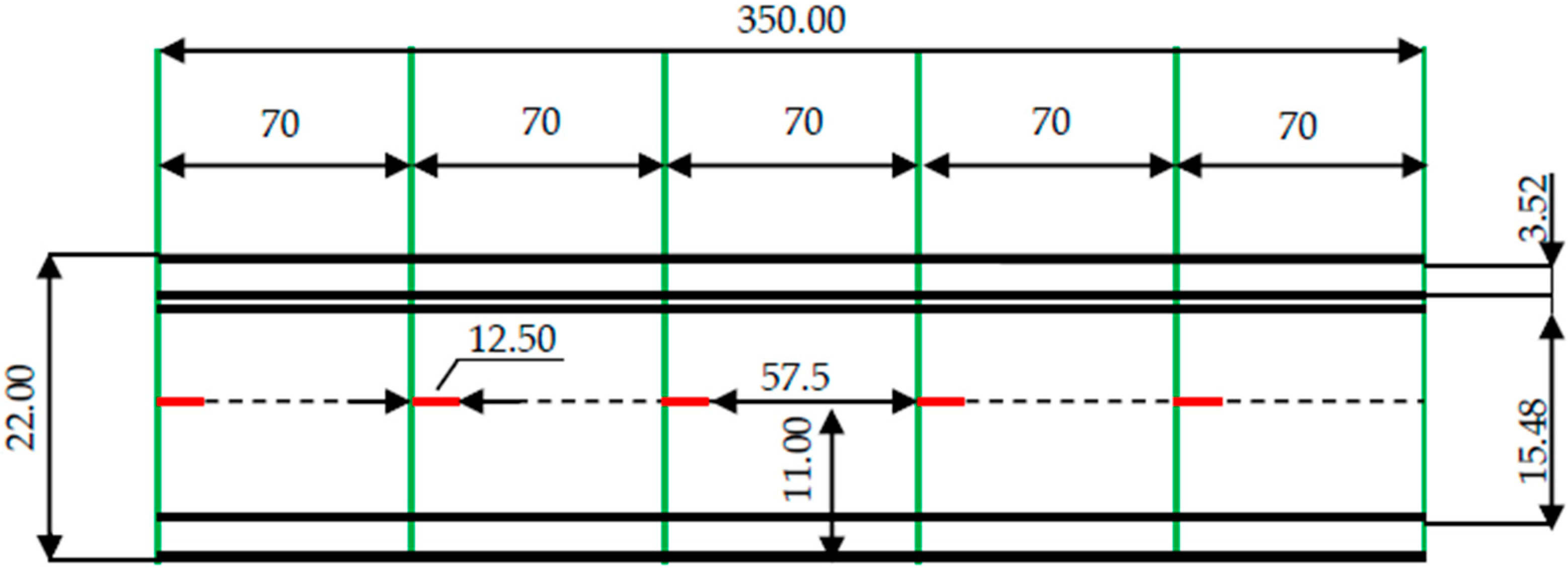
Figure 2.
CNC “Homag BOF 41/30/R”.

Figure 3.
Laser profile meter LPM 4.

Figure 4.
Residual analysis for Ra parameter (milling blade TO3SMG).

Table 1.
Variations of cutting speed and feed rate used in the experiment.
| Variant | vc [m·min−1] | vf [m·min−1] |
|---|---|---|
| 1. | 2513.27 | 4.00 |
| 2. | 3141.59 | 4.00 |
| 3. | 3769.91 | 4.00 |
| 4. | 4398.23 | 4.00 |
| 5. | 2513.27 | 8.00 |
| 6. | 3141.59 | 8.00 |
| 7. | 3769.91 | 8.00 |
| 8. | 4398.23 | 8.00 |
| 9. | 2513.27 | 10.00 |
| 10. | 3141.59 | 10.00 |
| 11. | 3769.91 | 10.00 |
| 12. | 4398.23 | 10.00 |
| 13. | 1884.96 | 4.00 |
| 14. | 1884.96 | 8.00 |
| 15. | 1884.96 | 10.00 |
| 16. | 4084.07 | 4.00 |
| 17. | 4084.07 | 8.00 |
| 18. | 4084.07 | 10.00 |
Table 2.
Measured and Calculated Values.
| Nr. | MRR [cm3·min−1] | V [cm3] | E [W] | Tf [min] | TL [min] | NO [EUR] | Ra [mm] |
|---|---|---|---|---|---|---|---|
| 1. | 407.56 | 101.890 | 101.7442 | 0.250 | 7.40 | 3.08 | 0.0114960 |
| 2. | 407.56 | 203.780 | 101.7442 | 0.250 | 4.61 | 4.79 | 0.0107695 |
| 3. | 407.56 | 305.670 | 101.7442 | 0.250 | 3.14 | 6.92 | 0.0118610 |
| 4. | 407.56 | 407.560 | 101.7442 | 0.250 | 2.26 | 9.48 | 0.0108260 |
| 5. | 815.12 | 509.450 | 50.87209 | 0.125 | 7.40 | 1.61 | 0.0143800 |
| 6. | 815.12 | 611.340 | 50.87209 | 0.125 | 4.61 | 2.46 | 0.0142430 |
| 7. | 815.12 | 713.230 | 50.87209 | 0.125 | 3.14 | 3.53 | 0.0125990 |
| 8. | 815.12 | 815.120 | 50.87209 | 0.125 | 2.26 | 4.81 | 0.0122090 |
| 9. | 1018.90 | 917.010 | 40.69767 | 0.100 | 7.40 | 1.31 | 0.0149325 |
| 10. | 1018.90 | 1018.900 | 40.69767 | 0.100 | 4.61 | 1.99 | 0.0134010 |
| 11. | 1018.90 | 1120.790 | 40.69767 | 0.100 | 3.14 | 2.85 | 0.0103585 |
| 12. | 1018.90 | 1222.680 | 40.69767 | 0.100 | 2.26 | 3.87 | 0.0114045 |
| 13. | 407.56 | 1324.570 | 101.7442 | 0.250 | 13.60 | 1.80 | 0.0118500 |
| 14. | 815.12 | 1426.460 | 50.87209 | 0.125 | 13.60 | 0.96 | 0.0129370 |
| 15. | 1018.90 | 1528.350 | 40.69767 | 0.100 | 13.60 | 0.80 | 0.0119000 |
| 16. | 407.56 | 1630.240 | 101.7442 | 0.250 | 2.65 | 8.14 | 0.0106670 |
| 17. | 815.12 | 1732.130 | 50.87209 | 0.125 | 2.65 | 4.14 | 0.0105500 |
| 18. | 1018.90 | 1834.020 | 40.69767 | 0.100 | 2.65 | 3.34 | 0.0112180 |
Table 3.
Regression analysis for the Ra parameter (milling blade T03SMG).
| N = 18 | b * | Standard Error for b * | b | Standard Error for b | t | Significance Value p |
|---|---|---|---|---|---|---|
| Absolute variables | 0.013598 | 0.001250 | 10.88250 | 3.25 × 10⁻⁸ | ||
| vc [m·min−1] | −0.450007 | 0.190930 | −6.84 × 10⁻⁷ | 2.90 × 10⁻⁷ | −2.35692 | 0.033519 |
| vf [m·min−1] | 0.531468 | 0.215402 | 0.000286 | 0.000116 | 2.46733 | 0.027123 |
| V [cm3] | −0.478004 | 0.215489 | −1.22 × 10⁻⁶ | 5.48 × 10⁻⁷ | −2.21823 | 0.043584 |
Table 4.
Outputs of trained and tested samples for roughness parameter Ra.
| Sample | vc [m·min−1] | vf [m·min−1] | V [cm3] | Ra-Median [mm] | Ra-Network [mm] | Deviation Ra |
|---|---|---|---|---|---|---|
| Test | 2513.27 | 4.00 | 101.890 | 0.011496 | 0.011787 | −2.53% |
| Train | 3141.59 | 4.00 | 203.780 | 0.010770 | 0.011775 | −9.34% |
| Train | 3769.91 | 4.00 | 305.670 | 0.011861 | 0.011740 | 1.02% |
| Train | 4398.23 | 4.00 | 407.560 | 0.012719 | 0.011683 | 8.15% |
| Train | 2513.27 | 8.00 | 509.450 | 0.014380 | 0.014230 | 1.04% |
| Test | 3141.59 | 8.00 | 611.340 | 0.014243 | 0.013610 | 4.45% |
| Train | 3769.91 | 8.00 | 713.230 | 0.012599 | 0.012939 | −2.70% |
| Train | 4398.23 | 8.00 | 815.120 | 0.012209 | 0.012297 | −0.72% |
| Train | 2513.27 | 10.00 | 917.010 | 0.014933 | 0.014984 | −0.35% |
| Train | 3141.59 | 10.00 | 1018.900 | 0.013401 | 0.013263 | 1.03% |
| Test | 3769.91 | 10.00 | 1120.790 | 0.010359 | 0.012040 | −16.23% |
| Train | 4398.23 | 10.00 | 1222.680 | 0.011405 | 0.011311 | 0.82% |
| Test | 1884.96 | 4.00 | 1324.570 | 0.011850 | 0.011574 | 2.33% |
| Train | 1884.96 | 8.00 | 1426.460 | 0.012937 | 0.012865 | 0.55% |
| Train | 1884.96 | 10.00 | 1528.350 | 0.013171 | 0.013231 | −0.45% |
| Test | 4084.07 | 4.00 | 1630.240 | 0.010667 | 0.011402 | −6.89% |
| Test | 4084.07 | 8.00 | 1732.130 | 0.010550 | 0.011319 | −7.29% |
| Test | 4084.07 | 10.00 | 1834.020 | 0.011218 | 0.010917 | 2.68% |
| Average of deviations absolute values | 3.81% | |||||
Table 5.
Outputs of trained and tested samples for operation costs NO.
| Sample | vc [m·min−1] | vf [m·min−1] | V [cm3] | NO-Calculation [€] | NO-Network [€] | Deviation NO |
|---|---|---|---|---|---|---|
| Test | 2513.27 | 4.00 | 101.890 | 3.08 | 2.95 | 4.47% |
| Train | 3141.59 | 4.00 | 203.780 | 4.79 | 4.78 | 0.22% |
| Train | 3769.91 | 4.00 | 305.670 | 6.92 | 7.00 | −1.26% |
| Train | 4398.23 | 4.00 | 407.560 | 9.48 | 9.37 | 1.16% |
| Train | 2513.27 | 8.00 | 509.450 | 1.61 | 1.60 | 0.82% |
| Test | 3141.59 | 8.00 | 611.340 | 2.46 | 2.43 | 1.07% |
| Train | 3769.91 | 8.00 | 713.230 | 3.53 | 3.59 | −1.91% |
| Train | 4398.23 | 8.00 | 815.120 | 4.81 | 5.01 | −4.22% |
| Train | 2513.27 | 10.00 | 917.010 | 1.31 | 1.21 | 8.08% |
| Train | 3141.59 | 10.00 | 1018.900 | 1.99 | 1.75 | 12.52% |
| Test | 3769.91 | 10.00 | 1120.790 | 2.85 | 2.62 | 8.05% |
| Train | 4398.23 | 10.00 | 1222.680 | 3.87 | 3.90 | −0.68% |
| Test | 1884.96 | 4.00 | 1324.570 | 1.80 | 1.27 | 29.36% |
| Train | 1884.96 | 8.00 | 1426.460 | 0.96 | 0.98 | −2.02% |
| Train | 1884.96 | 10.00 | 1528.350 | 0.80 | 0.90 | −12.82% |
| Test | 4084.07 | 4.00 | 1630.240 | 8.14 | 7.23 | 11.25% |
| Test | 4084.07 | 8.00 | 1732.130 | 4.14 | 4.43 | −7.08% |
| Test | 4084.07 | 10.00 | 1834.020 | 3.34 | 3.71 | −11.28% |
| Average of deviations absolute values | 6.57% | |||||
Table 6.
Outputs of trained and tested samples for total milling time Ts.
| Sample | vc [m·min−1] | vf [m·min−1] | V [cm3] | Ts-Calculation [min] | Ts-Network [min] | Deviation Ts |
|---|---|---|---|---|---|---|
| Test | 2513.27 | 4.00 | 101.890 | 0.517 | 0.515 | 0.36% |
| Train | 3141.59 | 4.00 | 203.780 | 0.517 | 0.517 | −0.09% |
| Train | 3769.91 | 4.00 | 305.670 | 0.517 | 0.518 | −0.20% |
| Train | 4398.23 | 4.00 | 407.560 | 0.517 | 0.517 | −0.04% |
| Train | 2513.27 | 8.00 | 509.450 | 0.392 | 0.391 | 0.06% |
| Test | 3141.59 | 8.00 | 611.340 | 0.392 | 0.391 | 0.14% |
| Train | 3769.91 | 8.00 | 713.230 | 0.392 | 0.390 | 0.34% |
| Train | 4398.23 | 8.00 | 815.120 | 0.392 | 0.389 | 0.62% |
| Train | 2513.27 | 10.00 | 917.010 | 0.367 | 0.372 | −1.47% |
| Train | 3141.59 | 10.00 | 1018.900 | 0.367 | 0.372 | −1.39% |
| Test | 3769.91 | 10.00 | 1120.790 | 0.367 | 0.371 | −1.28% |
| Train | 4398.23 | 10.00 | 1222.680 | 0.367 | 0.371 | −1.15% |
| Test | 1884.96 | 4.00 | 1324.570 | 0.517 | 0.497 | 3.73% |
| Train | 1884.96 | 8.00 | 1426.460 | 0.392 | 0.388 | 0.96% |
| Train | 1884.96 | 10.00 | 1528.350 | 0.367 | 0.371 | −1.28% |
| Test | 4084.07 | 4.00 | 1630.240 | 0.517 | 0.505 | 2.26% |
| Test | 4084.07 | 8.00 | 1732.130 | 0.392 | 0.386 | 1.46% |
| Test | 4084.07 | 10.00 | 1834.020 | 0.367 | 0.370 | −0.96% |
| Average of deviations absolute values | 0.99% | |||||
Table 7.
Optimal levels of setting cutting conditions considering the output parameters.
| vc [m·min−1] | N [rev·min−1] | vf [m·min−1] | Ra [µm] | Mark Ra | NO [€] | Mark NO | Ts [min] | Mark Ts |
|---|---|---|---|---|---|---|---|---|
| 1600.00 | 5093 | 3.00 | 10.375 | VL | 0.67 | VL | 0.534 | VH |
| 4398.23 | 14,000 | 11.00 | 10.548 | L | 3.64 | M | 0.373 | VL |
| 1600.00 | 5093 | 3.42 | 10.575 | L | 0.65 | VL | 0.515 | H |
| 4250.95 | 13,531 | 11.00 | 10.577 | L | 3.44 | M | 0.373 | VL |
| 4103.68 | 13,062 | 11.00 | 10.703 | L | 3.22 | M | 0.373 | VL |
| 1747.28 | 5562 | 3.00 | 10.748 | L | 1.04 | L | 0.538 | VH |
| 1600.00 | 5093 | 3.84 | 10.765 | L | 0.65 | VL | 0.497 | H |
| 4398.23 | 14,000 | 10.58 | 10.852 | L | 3.76 | M | 0.371 | VL |
| 4250.95 | 13,531 | 10.58 | 10.855 | L | 3.55 | M | 0.371 | VL |
| 3072.75 | 9781 | 3.00 | 10.928 | L | 5.30 | MH | 0.566 | VH |
| 1600.00 | 5093 | 4.68 | 11.116 | L | 0.64 | VL | 0.465 | MH |
| 1600.00 | 5093 | 5.11 | 11.278 | L | 0.64 | VL | 0.451 | MH |
| 1600.00 | 5093 | 4.26 | 10.945 | L | 0.64 | VL | 0.480 | MH |
| 1600.00 | 5093 | 5.53 | 11.429 | L | 0.65 | VL | 0.438 | M |
| 1600.00 | 5093 | 3.84 | 10.765 | L | 0.65 | VL | 0.497 | H |
| 1600.00 | 5093 | 5.95 | 11.571 | M | 0.65 | VL | 0.426 | L |
| 1600.00 | 5093 | 3.42 | 10.575 | L | 0.65 | VL | 0.515 | H |
| 1600.00 | 5093 | 6.37 | 11.704 | M | 0.66 | VL | 0.415 | L |
| 1600.00 | 5093 | 3.00 | 10.375 | VL | 0.67 | VL | 0.534 | VH |
| 1600.00 | 5093 | 6.79 | 11.826 | M | 0.68 | VL | 0.405 | L |
| 1600.00 | 5093 | 10.16 | 12.461 | M | 0.88 | VL | 0.369 | VL |
| 1600.00 | 5093 | 9.74 | 12.416 | M | 0.85 | VL | 0.369 | VL |
| 1600.00 | 5093 | 10.58 | 12.497 | M | 0.92 | VL | 0.369 | VL |
| 1747.28 | 5562 | 10.16 | 12.897 | MH | 0.89 | VL | 0.370 | VL |
| 4103.68 | 13,062 | 10.16 | 11.200 | L | 3.43 | M | 0.370 | VL |
| 4250.95 | 13,531 | 10.16 | 11.106 | L | 3.68 | M | 0.370 | VL |
| 1747.28 | 5562 | 10.58 | 12.936 | MH | 0.91 | VL | 0.371 | VL |
| 3956.40 | 12,594 | 10.16 | 11.454 | L | 3.13 | M | 0.371 | VL |
| 1747.28 | 5562 | 9.74 | 12.848 | MH | 0.88 | VL | 0.371 | VL |
| 4398.23 | 14,000 | 10.16 | 11.125 | L | 3.91 | M | 0.371 | VL |
N—spindle speed; Mark: VL—very low; L—low; M—middle; MH—medium high; H—high; VH—very high.
Table 8.
Optimal values.
| Inputs | ANN | Outputs | |||||
|---|---|---|---|---|---|---|---|
| vc [m·min−1] | N * [rev·min−1] | vf [m·min−1] | V [cm3] | Z | Ra [µm] | NO [EUR] | Ts [min] |
| 3072.75 | 9780.87 | 3.00 | 189.34 | 41.69 | 10.928 | 5.30 | 0.560 |
| 2925.48 | 9312.08 | 3.00 | 153.44 | 41.57 | 10.983 | 4.78 | 0.565 |
| 2483.65 | 7905.71 | 3.00 | 162.00 | 41.40 | 11.153 | 3.29 | 0.566 |
* N—spindle speed.
© 2017 by the authors. Licensee MDPI, Basel, Switzerland. This article is an open access article distributed under the terms and conditions of the Creative Commons Attribution (CC BY) license (http://creativecommons.org/licenses/by/4.0/).
Share and Cite
MDPI and ACS Style
Sujova, A.; Marcinekova, K.; Hittmar, S. Sustainable Optimization of Manufacturing Process Effectiveness in Furniture Production. Sustainability 2017, 9, 923. https://doi.org/10.3390/su9060923
AMA Style
Sujova A, Marcinekova K, Hittmar S. Sustainable Optimization of Manufacturing Process Effectiveness in Furniture Production. Sustainability. 2017; 9(6):923. https://doi.org/10.3390/su9060923
Chicago/Turabian StyleSujova, Andrea, Katarina Marcinekova, and Stefan Hittmar. 2017. "Sustainable Optimization of Manufacturing Process Effectiveness in Furniture Production" Sustainability 9, no. 6: 923. https://doi.org/10.3390/su9060923
Note that from the first issue of 2016, this journal uses article numbers instead of page numbers. See further details here.