Economic Transformation in the Beijing-Tianjin-Hebei Region: Is It Undergoing the Environmental Kuznets Curve?

Abstract

The Beijing-Tianjin-Hebei Region Integration Plan is one of the most important national strategies in China promoting regional economic development. The environmental problems in this region, however, especially air pollution and contaminated groundwater, have enormous influence on the people’s health while also causing economic loss. Therefore, this study aims to analyze the pattern of its environmental and economic development. Panel data in the period 2004–2014 are used to establish an advanced model of the Environmental Kuznets Curve. The results indicate that the economic growth and environmental pollution of Beijing-Tianjin-Hebei region do not completely meet the Environment Kuznets Curve assumptions. The discharge volume of industrial wastewater and economic growth reflect a wave-type relation. The sulfur dioxide discharge volume and economic growth reflect a U-shaped relation; the generated volume of industrial solid wastes and economic growth reflect a reversed N-shaped relation, which is in accordance with the Environmental Kuznets Curve characteristics at the second inflection point. The variables added value of the secondary industry, population size and raw coal consumption volume have a significant positive influence on the discharge of various environmental pollutants in Beijing-Tianjin-Hebei region. The analysis provides policy recommendations for the government to develop regional economic and environmental protection policies.

1. Introduction

The Beijing-Tianjin-Hebei (BTH) Region is one of the most important urban areas in China. The implementation of the BTH Regional Integration Strategy led the region’s total production output to exceed RMB 6.9 trillion by the end of 2015. It has become the third largest economic growth pole in China after the metropolitan regions of the Yangtze River Delta and Pearl River Delta [1,2]. However, the high-speed economic growth could never have been realized without extensive consumption of energy and resources. As an important high-tech and industrial base, the BTH region’s energy consumption has exceeded its environmental carrying capacity. Thus bringing a series of environmental problems, such as severe atmospheric pollution and underground water pollution. Studies have shown that, prior to the industrial revolution, humans probably had little impact, but human activities have caused some damage to the atmospheric environment after the industrial revolution, especially the use of fossil fuels, an increase in carbon dioxide emissions [3]. In November 2016, China’s State Council passed the “Ecological and Environmental Protection Plan of the Thirteenth Five Year Plan”, which indicated that the government shall comprehensively improve the emission standards and substantially reduce the discharge of pollutants during the “Thirteenth Five Year Plan” period. Following the experience of economically developed parts of the world, one would expect economic growth and environmental pollution reflecting a reversed U-shaped relation. This implies that the environment would gradually deteriorate with economic growth, but after economic development has reached a certain level, the environmental pollution would be reduced, in line with the so called “Pollution First, Treatment Later” creed [4,5,6,7]. However, whether the BTH region also follows that pattern (i.e., pollution first and treatment later) still requires empirical verification. Such an analysis would help in establishing appropriate policies based on an understanding of the relationship between environment and economy. Consequently, this research will first present a statistical description of changes in the economy and pollution levels in the BTH region. Subsequently, an improved model of the Environmental Kuznets Curve (EKC) will be used to implement a regression analysis based on province-level panel data of the region in the period 2004–2014. Based on an analysis of the curve shape, we will explain the underlying causes. At the end, policy recommendations will be provided for the economic transformation and the improvement of energy consumption structure of the BTH region.

There has been plenty of research regarding the relation between economic growth and the environment, of which a well-known example is the Environmental Kuznets Curve (EKC). EKC is based on empirical work conducted by the environmental economists Grossman and Kruger (1991, 1995) in their pioneering research [8,9]. Most of the studies on EKC theory hold that environmental quality will deteriorate at the early stages of economic development, while further down the road environmental quality will improve as the economy keeps growing [10]. Some scholars have used the EKC curve to study how economic growth can benefit environmental quality [11]. Some scholars based on the empirical research of Thailand and Malaysia find that GDP and export growth promote energy consumption and carbon dioxide emissions [12]. Other scholars have examined the impact of oil price changes on carbon dioxide emissions through EKC [13]. In addition, previous studies have suggested that the development of tourism industry is also an important factor of the quality of the environment [14,15,16]. Robalino-López et al. (2015) have argued that the relation between carbon dioxide emission (CO₂) volume and economic growth in 14 Asian countries reflects a reversed U-shaped relation, which is in conformity with the EKC theory [17]. Gupta (2015) used the EKC to establish the relation between income growth and use of fresh water resources [18]. The results indicated that the EKC theory applied to some countries, but not to others. The EKC’s applicability seems to depend on the actual circumstances of different countries and regions. In the case of Venezuela, long-term economic growth and environmental problems did not meet the EKC assumptions, but it showed a reversed U-shaped relation at the middle stage [19]. The government was advised to find the underlying causes of economic growth and environmental change during that reversed U-shaped period, and attach importance to adjust the energy structures during the economic transformation. When studying the relation between Gross Domestic Product (GDP) and CO₂ emission volume, Jebli et al. (2016) found that, apart from economic development, trade and the use of renewable energy also exerted obvious influence on environmental change [20]. Many countries now utilize renewable resources, but the effects of environmental improvement vary significantly. The environment in the US and Europe has improved, but the Middle East and some Asian countries have not made similar progress. Al-Mulali et al. (2016) have argued that the typical EKC assumption was met in the developed countries due to change in the energy structure underlying economic development [21]. It is far from certain whether the EKC assumption also helps to explain the situation in developing countries [22].

In China, the EKC theory assumption has also been widely discussed. Narayan (2010) adopted the quartic term relation of seven pollution indicators and per capita GDP to verify the EKC assumption for the city of Beijing. His results indicate that partial indicators met the assumption [23]. Jayanthakumaran (2012) used China’s province-level data and found that due to the unbalanced development among different regions, some pollution indicators failed to follow a decreasing trend when the economy kept growing [24]. The EKC curves of China’s northeast regions based on the method of the ecological footprint revealed that economic growth there was U-shaped in its resource consumption [25]. The EKC shapes of 47 Chinese prefecture-level resource-based cities were not completely similar to those of the nation as a whole [5]. The turning points for economic and environmental improvement in these resource-based cities appeared earlier than those elsewhere [26]. Feng et al. (2013) used a spatial econometric model with provincial panel data to study the EKC of China’s energy and electricity consumption [27]. Their results indicate that per capita GDP of energy consumption and electricity consumption is reversed N-shaped, in line with the EKC assumption. Many scholars have added control variables to study the relation between economic growth and pollution, for example for industrial structure, foreign trade volume, population size, energy consumption, technology progress and urbanization rate, all leading to more accurate explanations of the major causes behind environmental impact [28,29,30,31]. Existing studies mainly test the EKC of a region, a country or a group of countries in order to verify whether the relation between economic growth and environmental pollution follows a reversed U shape. Less attention is paid to considerations of regional integration. Moreover, most studies use fit tests with traditional quadratic terms and cubic terms of economic variables, which may not reflect the EKC’s distribution characteristics in real terms. Approaching the issue from an EKC perspective, in areas where government administrative intervention power is strong (the BTH region), the test whether EKC theory is effective and what it would be affected would provide corresponding empirical support for EKC theory. Here, based on insights from previous studies and with the perspective of BTH integration in mind, the quartic equation of economic variables will be applied and certain control variables added (including industrial structure, technology progress, population size, urbanization rate and energy consumption) to test whether the BTH region fits the EKC hypothesis.

2. Economic Growth and Environmental Pollution in the BTH Region

2.1. Overview of Economic Growth Rates

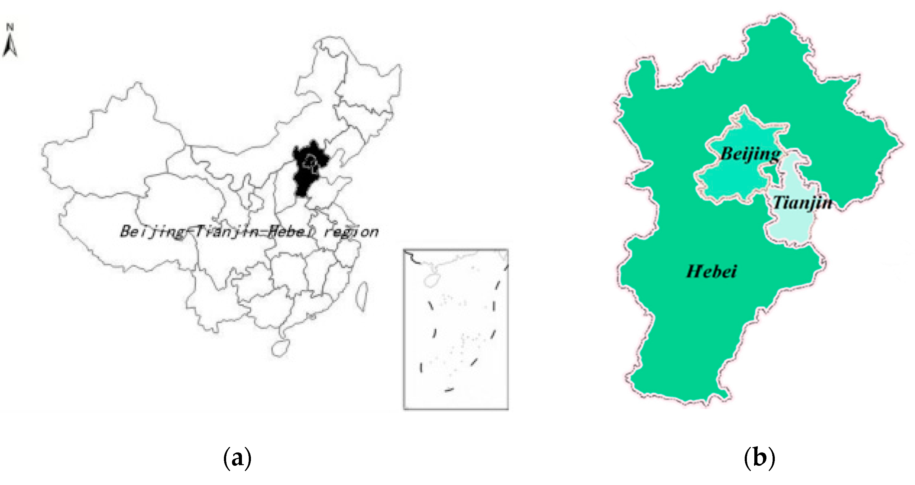
The BTH region is located on China’s northeastern coast and includes Beijing municipality. The population of BTH region is nearly 0.11 billion people in 2016, accounting for 8% of China’s total population. Tianjin municipality and Hebei province are shown in Figure 1.

Table 1. Per capita GDP growth rate (in %) in the BTH region 2004–2014.

-	2014	2013	2012	2011	2010	2009	2008	2007	2006	2005	2004	Average
B	6	8	7	11	10	4	7	16	12	12	17	10
T	5	7	9	17	17	7	22	14	11	24	20	14
H	3	6	8	18	17	7	17	16	14	18	22	13
Average	5	7	8	15	15	6	15	15	12	18	20	12

Note: Data Sources: China’s National Bureau of Statistics. B for Beijing; T for Tianjin; H for Hebei.

shows the growth rates of per capita GDP in the region in the period 2004–2014. The table shows that:

(1)

The overall per capita GDP in the BTH region reflected high growth rates from 2004 to 2011, except in 2009 when the annual average growth rate was lower than 10%. After 2012, growth rates remained all below double digits.

(2)

The annual average growth rate of per capita GDP in the BTH region exceeded 10%. The highest rate was obtained in Tianjin City (14%), followed by Hebei (13%), and the lowest was found for Beijing (10%).

(3)

The per capita growth rate in Beijing was generally stable over the years; the lowest growth rate was found for 2009 at 4% and the highest for 2004 at 17%; the lowest per capita GDP growth rate for Tianjin was found in 2014 at 5% and the highest in 2005 at 24%; and the lowest per capita growth rate in Hebei Province occurred in 2014 at 3% and the highest in 2004 at 22%. Moreover, in terms of GDP per capita in the entire BTH region, the year with the highest growth rate was 2004 (20%), and the lowest was 2014 (5%).

2.2. Overview of Environmental Emission Levels

Table 2. Growth Rates (in %) of discharge volumes of the “Three Wastes” in the BTH Region 2004–2014 (due to the loss of some data for the three types of environmental pollution indicators in 2003, the growth rate for 2004 remains empty).

-	-	2014	2013	2012	2011	2010	2009	2008	2007	2006	2005	Average
B	Water	4	3	−4	7	−3	24	5	3	4	3	4.6
	SO2	−9	−7	−4	−15	−3	−3	−19	−14	−7	−1	−8.2
	Solid	−2	−5	−2	−1	2	7	−9	−6	10	−5	−1.1
T	Water	6	2	23	−2	14	−3	8	−3	−3	24	6.6
	SO2	−4	−3	−3	−2	−1	−1	−2	−4	−4	17	−0.7
	Solid	9	−13	4	−6	23	2	6	8	15	49	9.7
H	Water	−1	2	10	6	7	4	5	4	2	1	4.0
	SO2	−7	−4	−5	14	−2	−7	−10	−3	3	5	−1.6
	Solid	−3	−5	1	42	44	11	6	31	−13	−3	11.1
Mean		−0.8	−3.3	2.2	4.8	9.0	3.8	−1.1	1.8	0.8	10.0	2.7

Note: B for Beijing; T for Tianjin; H for Hebei.

shows the growth rates in the discharge volume of industrial wastewater, SO₂ and industrial solid wastes in the BTH region in the years 2004–2014. As Table 2 shows:

(1)

From the perspective of overall growth, the discharge volume of the “Three Wastes” (wastewater, SO₂ and industrial solid wastes) in the BTH region generally reflects a decreasing trend. Some indicators (such as SO₂) already show negative growth, but a rebound in growth levels for some other indicators (such as wastewater) can be observed.

(2)

The growth rate in the “Three Wastes” volume by region shows that on average Beijing realized the lowest growth rate at 4.6%, −8.2% and −1.1%, respectively, while the average growth in Tianjin was the highest. Tianjin’s general growth rate in the “Three Wastes” discharge volume was 5.2%. The average growth in Hebei Province was higher than in Beijing, but lower than in Tianjin at 4.0%, −1.6% and 11.1%, respectively.

(3)

Considering the annual growth, the year with the highest average growth rate in the entire region was in 2005 at 10%, while the year with the lowest average growth was 2013 at −3.3%.

(4)

Regarding the structure of the growth rate, the discharge volumes of industrial wastewater and industrial solid waste were both relatively high: average growth in the discharge volume of industrial wastewater was 5.0%, and for generated volume of industrial solid waste, the growth rate was 6.6%. Negative growth was recorded for the discharge volume of industrial SO₂ with an average growth rate of −3.5%.

3. Method and Data

The previous section has briefly introduced the status quo of the BTH region’s economy and environment. It appears that a number of pollution indicators co-vary with economic growth and follow certain patterns. That is, pollution decreased as the economy kept growing. However, more detailed features still require rigorous testing to check whether they follow the assumptions underlying EKC theory. In this section, econometric methods will be adopted to unveil relations between environmental pollution and economic growth in the BTH region.

3.1. Moran Index

Based on the spatial effect theory in spatial econometrics, clarification of the correlation between inter-provincial economic development and pollutant discharge is required. Therefore, the study follows the method generally proclaimed in the literature by introducing the data of the spatial weight matrix to verify the spatial autocorrelation of the panel data. Spatial autocorrelation can be measured through the spatial autocorrelation index Moran’s I [32,33,34]; this study adopts “Local Moran’ s I”. The calculation formula reads as follows:

$$I_i=\frac{\left(x_i-\overline{x}\right)}{S^2}{\displaystyle {\sum }_{j=1}^n{w}_{ij}\left(x_j-\overline{x}\right)}$$

(1)

where S² is sample variance, W_ij is the (i, j) factor of the spatial weight matrix, and the value of Moran’s I is generally between −1 and 1. Positive I_i means that the high (low) value is encircled by the surrounding high (low) value; negative I_i means that the high (low) value of i in the area is encircled by the surrounding low (high) value [35,36,37].

Table 3. Spatial Autocorrelation Test (Moran’s I).

Variable	Province	Year	I	E (I)	SD (I)	Z	P
Discharge volume of industrial wastewater	Beijing	2004	−0.045	−0.500	0.354	1.288	0.198
		2014	−0.062	−0.500	0.354	1.240	0.215
	Tianjin	2004	−0.548	−0.500	0.354	−0.137	0.891
		2014	−0.511	−0.500	0.354	−0.032	0.975
	Hebei	2004	−0.907	−0.500	0.354	−1.150	0.250
		2014	−0.927	−0.500	0.354	−1.209	0.227
Emission volume of SO2	Beijing	2004	−0.272	−0.500	0.354	0.644	0.520
		2014	−0.348	−0.500	0.354	0.430	0.667
	Tianjin	2004	−0.228	−0.500	0.354	0.769	0.442
		2014	−0.163	−0.500	0.354	0.952	0.341
	Hebei	2004	−0.999	−0.500	0.354	−1.412	0.158
		2014	−0.988	−0.500	0.354	−1.382	0.167
Generated volume of industrial solid wastes	Beijing	2004	−0.449	−1.000	0.707	0.780	0.436
		2014	−0.527	−1.000	0.707	0.669	0.503
	Tianjin	2004	−0.553	−1.000	0.707	0.632	0.527
		2014	−0.474	−1.000	0.707	0.744	0.457
	Hebei	2004	−1.998	−1.000	0.707	−1.412	0.158
		2014	−2.000	−1.000	0.707	−1.414	0.157

reflects the tested value of local Moran’s I of the “Three Industrial Wastes” of BTH region. Due to considerations of article length, the table only includes the tested data in the first and last year. The test results show that there is no significant spatial autocorrelation between economic development and environmental pollution in the BTH region, perhaps due to the difference within the BTH region in terms of its industrial structure and production categories. Therefore, based on the test result, this study will continue to adopt the EKC model for empirical analysis.

3.2. Theoretical Model

As we know from existing research methods, with logarithmically processed data, severe fluctuation can be avoided without affecting the features of original data, while eliminating possible heteroscedasticity [38,39]. Therefore, this study employs the logarithmic model, assuming that there is quadruplicate relation between environmental pollution and economic growth in the BTH region. Four regression equations are established, respectively, by targeting the three pollution indicators. In the end, an optimal regression equation is adopted and the specific model is set as follows:

$$\ln Y_{it}={\alpha }_0+{\beta }_1\ln Pgd{p}_{it}+{\beta }_2\ln C_{it}+{\epsilon }_{it}$$

(2)

$$\ln Y_{it}={\alpha }_0+{\beta }_1\ln Pgd{p}_{it}+{\beta }_2\ln {(Pgd{p}_{it})}^2+{\beta }_3\ln C_{it}+{\epsilon }_{it}$$

(3)

$$\ln Y_{it}={\alpha }_0+{\beta }_1\ln Pgd{p}_{it}+{\beta }_2\ln {(Pgd{p}_{it})}^2+{\beta }_3\ln {(Pgd{p}_{it})}^3+{\beta }_4\ln C_{it}+{\epsilon }_{it}$$

(4)

$$\ln Y_{it}={\alpha }_0+{\beta }_1\ln Pgd{p}_{it}+{\beta }_2\ln {(Pgd{p}_{it})}^2+{\beta }_3\ln {(Pgd{p}_{it})}^3+{\beta }_4\ln {(Pgd{p}_{it})}^4+{\beta }_5\ln C_{it}+{\epsilon }_{it}$$

(5)

In Equations (1)–(4), α₀ means constant term; β means parameters to be estimated; ε means random disturbance term; and i, t, and Y represents province, year and pollution indicators, respectively, which include discharge volume of industrial wastewater, discharge volume of SO₂ and generated volume of industrial solid waste. The bigger the Y is, the more severe the pollution is. Pgdp means per capita GDP, which is the key explanatory variable. C stands for control variables made up by added value of secondary industry, population size, total import/export trade amount, urbanization rate, patent authorization, coal consumption volume, electricity consumption volume, and crude oil consumption volume.

Table 4. Explanation of the Variables.

Variables Type	Full Name	Standard Deviation	Abbreviation	Logarithmic
Dependent variables	discharge volume of industrial wastewater (Million tons)	83,880.29	Water	ln Water
	emission volume of SO2 (tons)	572,523.60	SO2	ln SO2
	generated volume of industrial solid wastes (Million tons)	14,958.69	Solid	ln Solid
Independent variables	per capita Gross Domestic Product (RMB)	27,792.23	Pgdp	ln Pgdp
Control variables	added value of secondary industry (Billion, RMB)	3913.95	Sgdp	ln Sgdp
	population size (Million)	2672.78	People	ln People
	total import/export trade amount (Billion, RMB)	1261.31	Trade	ln Trade
	urbanization rate (%)	19.14	City	ln City
	patent authorization	32,334.92	Tech	ln Tech
	coal consumption volume (Million tons)	11,115.39	Coal	ln Coal
	electricity consumption volume (Billion kwh)	930.16	Electricity	ln Electricity
	crude oil consumption volume (Million tons)	308.07	Crude	$\ln Crude$

shows the selection of the main indicators and introduces them briefly, mainly including the discharge volume of industrial wastewater, discharge volume of SO₂, generated volume of industrial solid waste, per capita GDP and related control variables. The selection of control variables refers to the previous literature and related theories. The added value of the secondary industry represents the degree and scale of industrial development. The higher its production output, the higher the corresponding discharge volume of “Three Industrial Wastes”; increasing population size leads to more pressure on the carrying capacity of the environment; the total amount of import/export trade correlates positively with external economic relation and the level of economic development; the urbanization rate has both negative and positive effects on environmental pollution indicators; regional scientific innovation capability is measured by the number of authorized patents which reflects the level of regional industrialization; and consumption indicators for coal, electricity and crude oil reflect regional energy consumption levels, positively related to discharge quantities of environmental pollutants.

Table 5. Evaluation Criteria for Economic Development and Environmental Pollution.

Number	β1	β2	β3	β4	Shape
1	β1 = 0	β2 = 0	β3 = 0	β4 = 0	Horizontal line
2	β1 < 0	β2 = 0	β3 = 0	β4 = 0	Monotonically decreasing
3	β1 > 0	β2 = 0	β3 = 0	β4 = 0	Monotonically increasing
4	β1 < 0	β2 > 0	β3 = 0	β4 = 0	“U” type
5	β1 > 0	β2 < 0	β3 = 0	β4 = 0	Inverted “U” type
6	β1 < 0	β2 > 0	β3 < 0	β4 = 0	Inverted “N” or “∽” type
7	β1 > 0	β2 < 0	β3 > 0	β4 = 0	“N” or “_” type
8	β4 ≠ 0				Wave type

Note: Based on the existing research.

shows the evaluation criteria for correlation (curve-shaped), mainly derived from existing EKC theory. More details are shown in Table 5.

Due to limited data availability, this study adopts panel data for the BTH region in the years 2004–2014. Data sources are mainly websites of China’s National Bureau of Statistics, China’s Environmental Statistical Yearbook, the Statistical Yearbook of Beijing City, the Statistical Yearbook of Tianjin City and the Statistical Yearbook of Hebei Province. The indicator for per capita GDP was adopted to reflect economic growth. Pollution in the BTH region is mainly caused by industrial production. Pollution indicators therefore include discharge volume of industrial wastewater, SO₂ emission volume, and generated volume of industrial solid waste. Based on the indicators issued by the Ministry of Environmental Protection and the experience in the literature [19,28,40,41,42,43], this study also adopts the related control variables such as the added value of the secondary industry, population size, total import/export trade amount, urbanization rate, patent authorization, coal consumption volume, electricity consumption volume and crude oil consumption volume. With these variables, we can increase the reliability and stability of the outcomes of the regression.

4. Results

4.1. Hausman Test

This study uses panel data for the BTH region in the years 2004–2014, and STATA13.0 for the regression analysis. The F test (p = 0.000 0) indicates that the fixed effect estimation is better than the combined OLS estimation. The Hausman test result (p = 0.290) is lower than the 0.05 default value of the STATA software, so the original assumption is rejected, and otherwise confirms the selection of the fixed effect model for the estimation. Through comparing the panel OLS, the fixed effect and the random effect regression, it was found that the coefficients obtained by panel OLS and stochastic effects underestimated the impact of per capita GDP and control variables on environmental pollution. The results of the specific panel OLS and random effects are shown in the Appendix A.

Table 6. Fixed effects regression results.

Variable Name	Discharge Volume of Industrial Wastewater	Emission Volume of SO2	Generated Volume of Industrial Solid Wastes
	Coefficient Standard Deviation	Coefficient Standard Deviation	Coefficient Standard Deviation
$\ln Pgdp$	−1469.2 **	−4.507 *	−4,697,267.3 ***
	(−2.37)	(−2.03)	(−2.90)
${(\ln Pgdp)}^2$	210.9 **	0.194 *	442,272.9 ***
	(2.37)	(1.84)	(2.93)
${(\ln Pgdp)}^3$	−13.40 **	-	−13,947.6 ***
	(−2.37)	-	(−2.93)
${(\ln Pgdp)}^4$	0.318 **	-	-
	(2.36)	-	-
$\ln Sgdp$	−0.225	0.616 **	13,637.4
	(−0.60)	(2.12)	(0.53)
$\ln People$	2.263 **	−1.938 ***	−81,260.5 *
	(2.70)	(−3.31)	(−1.79)
$\ln Trade$	−0.00246	−0.0625	5522.6
	(−0.03)	(−0.86)	(0.95)
$\ln City$	−0.828	−1.107	49,988.0
	(−1.12)	(−1.80)	(0.99)
$\ln Tech$	0.189 **	−0.0497	10,053.7 *
	(2.14)	(−0.72)	(1.87)
$\ln Coal$	0.288	0.701 ***	−3119.8
	(1.73)	(4.94)	(−0.27)
ln Electricity	−0.351	0.123	28,449.5
	(−0.80)	(0.33)	(0.96)
$\ln Crude$	−0.000805	−0.111	49.35
	(−0.01)	(−1.34)	(0.01)
_cons	3822.8 **	48.04 ***	16,728,648.5 ***
	(2.37)	(3.42)	(2.94)
Curve shape	Wave type	U type	inverted N type
R2	0.9515	0.9657	0.8689
LLC test	Adjusted t * (−0.44)	Adjusted t * (−2.08)	Adjusted t * (−3.41)
	p-value (0.0087)	p-value (0.0186)	p-value (0.0003)

Note: t statistics in parentheses * p < 0.1; ** p < 0.05; *** p < 0.01.

indicates the specific regression result, based on Equations of (2)–(5). The discharge volume of industrial wastewater, the SO₂ emission volume, the generated volume of industrial solid waste and per capita GDP were chosen to generate the optimal polynomial regression result, and the conclusions follow below.

4.2. EKC Test of the Discharge Volume of Industrial Wastewater and per Capita GDP

Based on the regression result, the equation expression of discharge volume of industrial wastewater and per capita GDP is:

$$\begin{array}{l}\ln Y_{it}={\alpha }_0-1469.2\ln Pgd{p}_{it}+210.9\ln {(Pgd{p}_{it})}^2-13.4\ln {(Pgd{p}_{it})}^3+\\ 0.318\ln {(Pgd{p}_{it})}^4+{\beta }_5\ln C_{it}+{\epsilon }_{it}\end{array}$$

(6)

Both the quadratic term and the cubic term for the discharge volume of industrial wastewater and per capita GDP of the BTH region failed to pass the test. The quartic term of per capita GDP is significant under the level of 5%, and it represents a positive correlation. R² is 0.9515 and the fit is relatively good. It is preliminary evidence that there may be quartic polynomial relation between economic growth and environmental pollution in the BTH region. We can conclude from the regression coefficient that the discharge volume of industrial wastewater and per capita GDP reflect a wave-shaped curve [44]. In addition, the discharge volume of industrial wastewater and per capita GDP are significantly below the 5% level representing a positive correlation; the discharge volume of industrial wastewater and the quantity of patent authorization are significant when they are below the 5% level, representing a positive correlation.

4.3. EKC Test of the Discharge Volume of SO₂ and per Capita GDP

Based on the regression result, we can conclude that the equation expression for the discharge volume of SO₂ and per capita GDP is:

$$\ln Y_{it}={\alpha }_0-4.507\ln Pgd{p}_{it}+0.194\ln {(Pgd{p}_{it})}^2+{\beta }_3\ln C_{it}+{\epsilon }_{it}$$

(7)

The discharge volume of SO₂ and per capita GDP reflect quadratic polynomial relation, which is relatively significant. R² is 0.9657, showing a relatively good fit. The quadratic term of per capita GDP is significant when it is below the 10% level, representing a positive correlation; we can conclude from the regression coefficient that the discharge volume of SO₂ and per capita GDP reflect a U-shaped curve. It indicates that with the increase in per capita GDP, the discharge volume of SO₂ first decreased before it increased, and the inflection point appeared around 2014. Before per capita GDP reached RMB 82,000, the pollution gradually improved, but afterwards the environmental pollution deteriorated again. In addition, the discharge volume of SO₂ and the added value of the secondary industry are significant when they are under the 5% level, representing a positive correlation; the discharge volume of SO₂ and population are significant under the 1% level, representing a negative correlation; the discharge volume and consumption volume of raw coal are significant under the 1% level, representing a positive correlation.

4.4. EKC Test of the Generated Volume of Industrial Solid Wastes and per Capita GDP

Based on the regression result, we can conclude that the equation expression between generated volume of industrial solid wastes and per capita GDP is:

$$\begin{array}{l}\ln Y_{it}={\alpha }_0-4,697,267.3\ln Pgd{p}_{it}+442,272.9\ln {(Pgd{p}_{it})}^2-\\ 13,947.6\ln {(Pgd{p}_{it})}^3+{\beta }_4\ln C_{it}+{\epsilon }_{it}\end{array}$$

(8)

The generated volume of industrial solid wastes and per capita GDP reflect a cubic polynomial relation, which is relatively significant at the level of 1%. R² is 0.8689, and the fit is relatively good; the generated volume of industrial solid wastes and per capita GDP reflect a reversed N-shaped curve, which is in accordance with the EKC assumption. It indicates that with the growth of the economy, the generated volume of industrial solid wastes in the BTH region increased before it decreased. The calculated two turning points are when the total amount reaches RMB 36,919 in 2006 and RMB 72,411 in 2012, respectively. In addition, the generated volume of industrial solid wastes and population size are significant when they are below the 10% level, representing a negative correlation; the generated volume of industrial solid wastes and number of authorized patents are significant when they are under the 10% level, representing a positive correlation.

Since the data are long panel data, the unit root test can be done by LLC test. The statistics are shown in table. The adjusted t* is significantly negative and p-value is smaller than 0.05, which means that the original assumptions of unit roots of panel data are rejected, therefore, panel data is stable.

5. Discussion

The current levels of industrial wastewater discharge and economic growth in the BTH region do not yet meet the EKC assumption, as appears from the results of EKC model test. The discharge volume of industrial wastewater continues to grow rapidly most of the time. Besides, from the regression results: the discharge of industrial wastewater is influenced by population size and the application newly patently technologies. The higher the population, the more industrial activity is needed, and the more the environmental carrying capacity is negatively affected.

The consumption volume of raw coal has major effect on the discharge volume of SO₂, indicating that raw coal is also an important source of SO₂ pollution [45]; the added value of the secondary industry also has a certain influence on SO₂ discharge, which suggests that industrial production is the direct cause of increases in SO₂; and the increase in the population size also has significant influence on SO₂ emissions. Usually, cities and regions with medium-sized populations have bigger size of industrial development, because the medium-sized cities in China are still in the industrial expansion stage, and have not yet reached the post-industrialization. As a result, those cities or regions discharge relatively more SO₂.

As for the generated volume of industrial solid waste, we can see that in the EKC test result that when per capita GDP is lower than RMB 36,919, the generated volume of industrial solid waste and per capita GDP show a monotone decrease; when per capita GDP is higher than RMB 36,919 and lower than RMB 72,411. Behind the economic growth we apparently find a trend of year-after-year increases in the generated volume of industrial solid waste [46]. Besides, the population growth seems to lead to lower volumes of industrial solid wastes, perhaps to be explained by the relatively limited expansion of new industrial construction in the metropolis in recent years. The volume in new patent application also has a certain influence on the generated volume of industrial solid wastes, which is contradictory to what is found in some earlier literature [47,48]. This is evidence that technological progress has two different possible consequences for environmental pollution: it either relieves environmental pressure or intensifies it. We must therefore conclude that the effects of new technologies require more in-depth study.

6. Conclusions

In April 2015, the “Planning Guideline of the Coordinated Development of BTH Region” was passed. The Chinese Government has clearly confirmed that the economic development of BTH Region is a key national strategy. However, environmental problems have also become increasingly severe as a direct consequence of this same rapid economic growth. This study gives evidence that the physical environment in the BTH Region is clearly deteriorating. The “Three Industrial Wastes” appear from it as the main sources of the pollution, in line with what can be observed in daily life.

Our main findings can be summarized as follows:

(1)

The discharge volume of industrial wastewater and economic growth reflect a wave-shaped relation, indicating that wastewater discharge fluctuates along with economic growth. Discharge volumes continue to rise and do not decrease as the economy grows.

(2)

The emission volume of SO₂ and economic growth show a U-shaped relation, indicating that the emission volume of SO₂ decrease first before it increase again as the economy grows.

(3)

The relation between generated volume of industrial solid wastes and economic growth is reversed N-shaped; this conforms with the EKC features below the second inflection point. Here, discharge volume gradually decreases as the economy grows.

(4)

The added value of the secondary industry, population size and the consumption volume of raw coal have clear influence on the environmental pollution in the BTH region, and lead to increases in the discharge of the “Three Industrial Wastes”. It needs to be added here that gross industrial and economic growth is not the single determinant of environmental pollution, because various external factors come into play, such as geographic location, climate, and agricultural production.

We must conclude that economic growth and environmental pollution in the BTH region do not completely follow the patterns predicted by the Environmental Kuznets Curve. Consequently, the comfortable idea that “Pollution before Treatment” can work for the economic transformation in the BTH region is illusory. Urbanization in the BTH region can be most effectively improved by targeting population size and raw coal consumption. Moreover, local governments can focus on promoting the economic integration of the three areas and enhancing resource distribution efficiency. Finally, the energy consumption structure can be adjusted, with the aim to gradually reduce the consumption of traditional energy such as coal and oil, and actively popularize clean energy and develop transport modes relying on renewables.

Hebei is obviously not at the same stage as Beijing and Tianjin in terms of its economic development. The share of the secondary industry to Hebei’s GDP is much higher, causing high discharge volumes for the three types of waste. Geographically, Beijing and Tianjin are mostly surrounded by Hebei; therefore, its pollution significantly affects Beijing and Tianjin, especially atmospheric pollution. Finding an ecological compensation model among the three areas may be due to healthy coordinated development.

Due to the limitations of the data, this paper only examines the relationship between the three types of environmental pollutants and economic growth. With the further disclosure of data and updating of the method, more environmental pollution indicators will be added to further test the EKC theory in Beijing-Tianjin-Hebei.

References

- Wang, S.J.; Ma, H.; Zhao, Y.B. Exploring the relationship between urbanization and the eco-environment—A case study of Beijing-Tianjin-Hebei region. Ecol. Indic. 2014, 45, 171–183. [Google Scholar] [CrossRef]
- Wu, D.; Xu, Y.; Zhang, S. Will joint regional air pollution control be more cost-effective? An empirical study of China’s Beijing–Tianjin–Hebei region. J. Environ. Manag. 2015, 149, 27–36. [Google Scholar] [CrossRef] [PubMed]
- Dergiades, T.; Kaufmann, R.K.; Panagiotidis, T. Long-Run Changes in Radiative Forcing and Surface Temperature: The Effect of Human Activity over the Last Five Centuries. J. Environ. Manag. 2016, 76, 67–85. [Google Scholar] [CrossRef]
- Dijkgraaf, E.; Vollebergh, H.R.J. A Test for Parameter Homogeneity in CO2 Panel EKC Estimations. Environ. Res. Econ. 2005, 32, 229–239. [Google Scholar] [CrossRef]
- Jalil, A.; Mahmud, S.F. Environment Kuznets curve for CO2 emissions: A cointegration analysis for China. Energ. Policy 2009, 37, 5167–5172. [Google Scholar] [CrossRef]
- Al-Rawashdeh, R.; Jaradat, A.Q.; Al-Shboul, M. Air Pollution and Economic Growth in MENA Countries: Testing EKC Hypothesis. Environ. Res. Eng. Manag. 2015, 70. [Google Scholar] [CrossRef]
- Bimonte, S.; Stabile, A. Land consumption and income in Italy: A case of inverted EKC. Ecol. Econ. 2017, 131, 36–43. [Google Scholar] [CrossRef]
- Fan, J.; Hu, H. Studies and Applications of Environmental Kuznets Curve (EKC). Math. Pract. Theory 2002, 6, 944–951. [Google Scholar]
- Esteve, V.; Tamarit, C. Is there an environmental Kuznets curve for Spain? Fresh evidence from old data. Econ. Model. 2012, 29, 2696–2703. [Google Scholar] [CrossRef]
- Dinda, S. Environmental Kuznets Curve Hypothesis: A Survey. Ecol. Econ. 2004, 49, 431–455. [Google Scholar] [CrossRef]
- Farhani, S.; Mrizak, S.; Chaibi, A.; Rault, C. The environmental Kuznets curve and sustainability: A panel data analysis. Energy Policy 2014, 71, 189–198. [Google Scholar] [CrossRef]
- Anatasia, V. The causal relationship between GDP, exports, energy consumption, and CO2 in Thailand and Malaysia. Int. J. Econ. Perspect. 2015, 9, 37–48. [Google Scholar]
- Katircioglu, S. Investigating the Role of Oil Prices in the Conventional EKC Model: Evidence from Turkey. Asian Econ. Financ. Rev. 2017, 7, 498–508. [Google Scholar]
- Katircioglu, S.T. Testing the Tourism-Induced EKC Hypothesis: The Case of Singapore. Econ. Model. 2014, 41, 383–391. [Google Scholar] [CrossRef]
- Katircioglu, S.T. International Tourism, Energy Consumption, and Environmental Pollution: The Case of Turkey. Renew. Sustain. Energy Rev. 2014, 36, 180–187. [Google Scholar] [CrossRef]
- Katircioglu, S.T.; Feridun, M.; Kilinc, C. Estimating Tourism-Induced Energy Consumption and CO2 Emissions: The Case of Cyprus. Renew. Sustain. Energy Rev. 2014, 29, 634–640. [Google Scholar] [CrossRef]
- Robalino-López, A.; Mena-Nieto, Á.; García-Ramos, J.E.; Golpe, A.A. Studying the relationship between economic growth, CO2 emissions, and the environmental Kuznets curve in Venezuela (1980–2025). Renew. Sustain. Energy Rev. 2015, 41, 602–614. [Google Scholar] [CrossRef]
- Gupta, J. Normative Issues in Global Environmental Governance: Connecting Climate Change, Water and Forests. J. Agric. Environ. Ethics 2015, 28, 413–433. [Google Scholar] [CrossRef]
- Apergis, N.; Ozturk, I. Testing Environmental Kuznets Curve hypothesis in Asian countries. Ecol. Indic. 2015, 52, 16–22. [Google Scholar] [CrossRef]
- Jebli, M.B.; Youssef, S.B.; Ozturk, I. Testing environmental Kuznets curve hypothesis: The role of renewable and non-renewable energy consumption and trade in OECD countries. Ecol. Indic. 2016, 60, 824–831. [Google Scholar] [CrossRef]
- Al-Mulali, U.; Ozturk, I.; Solarin, S.A. Investigating the environmental Kuznets curve hypothesis in seven regions: The role of renewable energy. Ecol. Indic. 2016, 67, 267–282. [Google Scholar] [CrossRef]
- Hamit-Haggar, M. Greenhouse gas emissions, energy consumption and economic growth: A panel cointegration analysis from Canadian industrial sector perspective. Energy Econ. 2012, 34, 358–364. [Google Scholar] [CrossRef]
- Narayan, P.K.; Narayan, S. Carbon dioxide emissions and economic growth: Panel data evidence from developing countries. Energy Policy 2010, 38, 661–666. [Google Scholar] [CrossRef]
- Jayanthakumaran, K.; Liu, Y. Openness and the Environmental Kuznets Curve: Evidence from China. Econ. Model. 2012, 29, 566–576. [Google Scholar] [CrossRef]
- Fu, W.; Zhao, J.Q.; Du, G.Z. Ecological Safety Analysis of the Northwest Region of China Based on the Ecological Footprint and Environmental Kuznets Curve. China Popul. Resour. Environ. 2013, 23, 107–110. [Google Scholar]
- Pasten, R.; Figueroa, E. The Environmental Kuznets Curve: A Survey of the Theoretical Literature. Int. Rev. Environ. Resour. Econ. 2012, 6, 195–224. [Google Scholar] [CrossRef]
- Feng, Y.Y.; Chen, S.Q.; Zhang, L.X. System dynamics modeling for urban energy consumption and CO2 emissions: A case study of Beijing, China. Ecol. Model. 2013, 252, 44–52. [Google Scholar] [CrossRef]
- Pedroni, P. Panel Cointegration: Asymptotic and Finite Sample Properties of Pooled Time Series Tests With an Application to the PPP Hypothesis. Econom. Theor. 2004, 20, 597–625. [Google Scholar] [CrossRef]
- Jaunky, V.C. The CO2 emissions-income nexus: Evidence from rich countries. Energy Policy 2011, 39, 1228–1240. [Google Scholar] [CrossRef]
- Arouri, M.E.H.; Youssef, A.B.; M’Henni, H.; Rault, C. Energy consumption, economic growth and CO2 emissions in Middle East and North African countries. Energy Policy 2012, 45, 342–349. [Google Scholar] [CrossRef]
- Pietrosemoli, L.; Monroy, C.R. The impact of sustainable construction and knowledge management on sustainability goals. A review of the Venezuelan renewable energy sector. Renew. Sustain. Energy Rev. 2013, 27, 683–691. [Google Scholar] [CrossRef]
- Nelson, G.C.; Hellerstein, D. Do Roads Cause Deforestation? Using Satellite Images in Econometric Analysis of Land Use. Am. J. Agric. Econ. 1997, 79, 80–88. [Google Scholar] [CrossRef]
- Anselin, L.; Bongiovanni, R.; Lowenbergdeboer, J. A Spatial Econometric Approach to the Economics of Site-Specific Nitrogen Management in Corn Production. Am. J. Agric. Econ. 2004, 86, 675–687. [Google Scholar] [CrossRef]
- Autant-Bernard, C.; Lesage, J.P. Quantifying Knowledge Spillovers Using Spatial Econometric Models. J. Reg. Sci. 2011, 51, 471–496. [Google Scholar] [CrossRef]
- Henry, M.S.; Schmitt, B.; Piguet, V. Spatial Econometric Models for Simultaneous Systems: Application to Rural Community Growth in France. Int. Reg. Sci. Rev. 2001, 24, 171–193. [Google Scholar] [CrossRef]
- Dall’Erba, S.; Gallo, J.L. Regional convergence and the impact of European structural funds over 1989–1999: A spatial econometric analysis. Pap. Reg. Sci. 2008, 87, 219–244. [Google Scholar] [CrossRef]
- Breustedt, G.; Habermann, H. The Incidence of EU Per-Hectare Payments on Farmland Rental Rates: A Spatial Econometric Analysis of German Farm-Level Data. J. Agric. Econ. 2011, 62, 225–243. [Google Scholar] [CrossRef]
- Och, F.J.; Ney, H. A systematic comparison of various statistical alignment models. Comput. Linguist. 2003, 29, 19–51. [Google Scholar] [CrossRef]
- Wooldridge, J.M. Cluster-Sample Methods in Applied Econometrics. Am. Econ. Rev. 2003, 93, 133–138. [Google Scholar] [CrossRef]
- Westerlund, J. Testing for Error Correction in Panel Data. Oxf. Bull. Econ. Stat. 2007, 69, 709–748. [Google Scholar] [CrossRef]
- Atici, C. Carbon emissions in Central and Eastern Europe: Environmental Kuznets curve and implications for sustainable development. Sustain. Dev. 2009, 17, 155–160. [Google Scholar] [CrossRef]
- Kleemann, L.; Abdulai, A. The Impact of Trade and Economic Growth on the Environment: Revisiting the Cross-Country Evidence. J. Int. Dev. 2013, 25, 180–205. [Google Scholar] [CrossRef]
- Shafiei, S.; Salim, R.A. Non-renewable and renewable energy consumption and CO2 emissions in OECD countries: A comparative analysis. Energy Policy 2014, 66, 547–556. [Google Scholar] [CrossRef]
- Yang, H.; He, J.; Chen, S. The fragility of the Environmental Kuznets Curve: Revisiting the hypothesis with Chinese data via an “Extreme Bound Analysis”. Ecol. Econ. 2015, 109, 41–58. [Google Scholar] [CrossRef]
- Shi, Q.; Deng, X.; Shi, C.; Chen, S. Exploration of the Intersectoral Relations Based on Input-Output Tables in the Inland River Basin of China. Sustainability 2015, 7, 4323–4340. [Google Scholar] [CrossRef]
- Wu, R.; Zhang, J.; Bao, Y.; Zhang, F. Geographical Detector Model for Influencing Factors of Industrial Sector Carbon Dioxide Emissions in Inner Mongolia, China. Sustainability 2016, 8, 149. [Google Scholar] [CrossRef]
- Stanton, E.A. The Tragedy of Maldistribution: Climate, Sustainability, and Equity. Sustainability 2012, 4, 394–411. [Google Scholar] [CrossRef]
- Wübbeke, J.; Heroth, T. Challenges and political solutions for steel recycling in China. Resour. Conserv. Recycl. 2014, 87, 1–7. [Google Scholar] [CrossRef]
Figure 1.
The BTH region: (a) The BTH region is located on China’s northeastern coast. (b) The BTH region includes Beijing municipality, Tianjin municipality and Hebei province.