
Eco-Efficiency Evaluation Considering Environmental Stringency


1
Korea E-Trade Research Institute, Chung-Ang University, Seoul 06974, Korea
2
School of Business Administration, College of Business and Economics, Chung-Ang University, Seoul 06974, Korea
*
Author to whom correspondence should be addressed.
Sustainability 2017, 9(4), 661; https://doi.org/10.3390/su9040661
Submission received: 22 February 2017
/
Revised: 3 April 2017
/
Accepted: 13 April 2017
/
Published: 21 April 2017
(This article belongs to the Special Issue Advances in Multiple Criteria Decision Making for Sustainability: Modeling and Applications)
Abstract
:This paper proposes an extended data envelopment analysis (DEA) model for deriving eco-efficiency. In order to derive eco-efficiency, the proposed model utilizes the concepts of operational efficiency and environmental efficiency. Since DEA can separately measure operational efficiency and environmental efficiency, the treatment for constructing the unified indicator is required to ultimately evaluate eco-efficiency through balancing operational and environmental concerns. To achieve this goal, we define the environmental stringency as the business condition reflecting the degree of enforcing environmental regulations across the firms or particular industries in different countries. The proposed model provides flexibility, as required by the pollution-intensity of industry, in that it allows the decision maker to evaluate DMU’s (decision-making unit) eco-efficiency appropriately depending on the business environment. We present a case of agricultural production systems to help readers understand what eco-efficiency becomes when we vary the stringency conditions. Through the illustrative example, this paper presents the potential application by which different environmental stringencies can successively be incorporated in DEA.
1. Introduction
Recently, sustainability has become an undoubtedly critical issue, and many researchers involved in environment studies have been paying serious attention to the challenging topic in order to achieve both economic and environmental goals. Since the concept of eco-efficiency was first proposed by Schaltegger and Sturm [1], a number of researchers as well as organizations suggested their own definitions and also tried to link business with environmental issues, ultimately for sustainability. For example, according to the World Business Council for Sustainable Development, eco-efficiency is achieved by “the delivery of competitively priced goods and services that satisfy human needs and bring quality of life, while progressively reducing ecological impacts and resource intensity throughout the life cycle, to a level at least in line with the earth’s carrying capacity” [2]. Although the definitions are slightly different, in essence they have the common core that eco-efficiency means to “efficiently produce with less pollutants and energy”. Obviously, it is worth noting that the major concern of measuring eco-efficiency is on how to improve economic performance while diminishing environmental damages. So, currently, eco-efficiency is of high concern in many business areas.
Data envelopment analysis (DEA), first proposed by [3], is an effective tool in evaluating the efficiencies of a set of decision-making units (DMUs), which use multiple inputs to produce multiple outputs. DEA does not require the parametric specifications of a particular function and it also does not require the predetermined weights to be attached to each input and output. Since the original model was carried out, many researchers have contributed to the refinement and extension of DEA for the various fields of their interests. Traditional DEA models allow the users to evaluate the economic performance of individual DMUs, depending on a profitability perspective. However, because addressing the environmental performance of organizations has become one of the important issues, it is necessary to extend the present DEA techniques or develop new DEA techniques that take into account environmental impacts on the performance evaluation.
Over the past two decades, the efforts for environmental application using DEA have increased considerably (e.g., [4,5,6,7,8,9,10,11,12,13,14,15,16,17,18,19,20,21,22]). In general, the efficiency is derived from a fractional formulation that either minimizes inputs while holding outputs constant or maximizes outputs while holding inputs constant. Also, there are other approaches for maximizing outputs and minimizing inputs simultaneously. Under these optimization schemes, the result of DEA is directly affected by clearly defined input and output variables. Therefore, the inputs and outputs should be selected for a particular problem context. However, in the production process, traditional DEA models cannot provide accurate results if there are important variables that have a negative effect on the environment. Such environmentally detrimental factors can be considered undesirable outputs, which are often produced along with desirable outputs and are expected to be minimized. As Färe et al. [23] pointed out, the performances of DMUs turn out to be very sensitive to whether or not undesirable outputs are included. There are DEA studies that tried to incorporate undesirable outputs. For example, Färe and Grosskopf [24], Seiford and Zhu [25], and Liu et al. [26] clarified the issue of efficiency evaluation of undesirable outputs and provided the mathematical models to solve it.
Usually, the performance measure incorporating both desirable and undesirable outputs is used as a form of environmental efficiency in environment studies. Since DEA can separately measure the operational (technical) and environmental efficiency, the treatment for constructing the unified measure is required to ultimately evaluate eco-efficiency through balancing operational and environmental concerns. Among the aforementioned environmental studies, Korhonen and Luptacik [6], Zhang et al. [20], and Mahdiloo et al. [8] provided the DEA-based eco-efficiency models considering environmental variables by setting them to undesirable outputs. To derive eco-efficiency, they used an environmental efficiency (ecological efficiency) measure as the ratio of undesirable outputs to desirable outputs and combined it with traditional operational efficiency, defined as the ratio of desirable outputs to inputs. That is, the undesirable outputs behave like inputs for environmental efficiency calculation. Mahdiloo et al. [8] criticized the so-called three-step methods, suggested by [6,20], in that the combination of operational and environmental efficiency does not provide a valid eco-efficiency score. Furthermore, Mahdiloo et al. [8] suggested multiple objective linear programming (MOLP) to incorporate technical and environmental efficiency so as to reduce the computational burden resulting from the three-step methods. The MOLP model recognizes DMUs as being eco-efficient if and only if they are both operationally and environmentally efficient, while the former models identify them if a DMU is either operationally or environmentally efficient.
In this research, a modified DEA model is suggested for taking into account the environment-related factors. Along this line of research, this study attempts to determine eco-efficiency on the basis of the operational and environmental aspects without directly unifying both operational and environmental efficiency. In order to reflect environmental concern across business situations, we propose a new model with parametric constraints that represent the situational context of environmental concern. As pointed out by [6], studies on the impact of environmental policy on the efficiency measure across the firms or particular industries in different countries are required. Our research aimed at addressing this challenge.
To show applicability, agricultural production systems are illustrated by a new model suggested in this research. That is, we apply the modified DEA model to soybean data gathered from 94 farms in Iran. Recently, many agricultural applications have been examined to derive eco-efficiency using DEA methodology, focusing on regional specific evaluation (China [27], Canada [28], Iran [29], Japan [30], Spain [31]). In addition, other applications for eco-efficiency are employed for the evaluation of factories [4,9,15,19], power plants [6,10,14,18,32], supplier selection [8], regions and cities [7,12,13,16,17,21], and transportation [33]. Particularly, unlike previous studies, we present a generalized way to evaluate any condition with regard to the different levels of environmental pressures or environmental concerns.
The remainder of this paper is organized as follows. In Section 2, DEA formulations of operational and environmental efficiency are introduced with input decomposition. Also, the proposed model for eco-efficiency is presented. In Section 3, we illustrate the proposed method using soybean data collected from 94 farms in Iran. Finally, conclusions are given in Section 4.
2. Proposed Method
The conceptual DEA framework of eco-efficiency evaluation for sustainability is depicted in Figure 1.
Consistent with previous studies [6,20], the underlying eco-efficiency of the proposed model is based on the idea that undesirable outputs can be treated as inputs in a fractional form for efficiency calculation.
2.1. Input Decomposition
As a preliminary work, we decompose inputs in the proposed DEA model into two types, which are operational inputs and environmental inputs. Operational inputs consist of labor, machinery, resources, energy, etc. In some DEA studies, energy has evolved as an important measurement, and it has been widely investigated not only as an energy efficiency measurement [34,35,36] but also as an input variable [8,20]. Since our study is not limited to the efficient use of energy, the proposed model considers it as an input variable along with traditional inputs such as labor, machinery, and resources. It is reasonable to consider the energy (e.g., electricity, gasoline, diesel, natural gas, and so on) as an input because it is a key and basic resource in most production processes. Environmental inputs are defined as undesirable outputs, e.g., emission of CO2, SO2, or NO, which are generated from the entire production process. In this study, the life cycle inventory (LCI) information, which describes all the resources used and all the emissions released into the environment connected with the production process, is employed to determine environmental inputs more specifically.
2.2. Operational Efficiency
In general, the operational efficiency accounts for the capability of an organization that produces products or services in a cost-effective manner while ensuring the quality. Typically, it is defined as the ratio of the outputs to the inputs in a system. Thus, we define operational efficiency as the ratio of desirable outputs to operational inputs.
The traditional DEA model is the basis for developing a new model for eco-efficiency. This model implicitly assumes that all DMUs operate a constant returns to scale (CRS) transformation of the inputs into outputs. We adopt a CRS assumption in this study. When there are m operational inputs (i = 1, 2, …, m) and s outputs (r = 1, 2, …, s) for each DMU j (j = 1, 2, …, n), the operational efficiency of a particular DMU o can be formulated as the following fractional programming model:
where vi and ur are unknown non-negative weights for operational inputs and outputs, respectively. Also, Model (1) can be transformed into a linear model through the Charnes-Cooper transformation [37]:
If the optimal value of the objective function in Model (2) equals to one, then it can be said of the specific DMU o that it is on the efficient frontier.
2.3. Environmental Efficiency
Compared to operational efficiency, environmental efficiency explains how efficiently produced the outputs are relative to the environmental inputs, as defined above. Thus, environmental efficiency is calculated as the ratio of outputs to environmental inputs. Assume there are p environmental inputs (k = 1, 2, …, p) for each DMU j (j = 1, 2, …, n), the environmental efficiency of a particular DMU o can be formulated as follows:
Model (3) also can be transformed to a linear model using the Charnes-Cooper transformation as follows:
2.4. A Model for Eco-Efficiency
At this stage, we proposed a more concrete DEA method for eco-efficiency using both operational and environmental efficiency simultaneously. If there are m operational inputs and p environmental inputs, the total weighted sum of the inputs to a DMU j can be calculated as . Thus, eco-efficiency incorporating operational and environmental impacts on the process performance could be expressed as the ratio of the weighted sum of outputs to the weighted sum of total inputs. Accordingly, the eco-efficiency of a particular DMU o is formulated as follows:
In Model (5), the parameter δ reflects environmental regulation in a particular production problem. That is, in order for the decision maker to respond appropriately to a given situation, the parameter plays an adjusting role toward operational or environmental orientation. Specifically, the smaller δ explains the situation that focuses more on the operational excellence, while the larger δ implies the higher environment pressure that exists in the industry. Thus, we call this parameter δ the degree of environmental stringency that explains environmental sensitivity.
Also, this model is a generalized version of [6,20] because the two models lead to identical outcomes to the proposed model if δ = 1. This parameter illustrates the relative importance between operational and environmental inputs and is specified by the decision maker. By assigning the approporiate value to δ, the evaluation method for eco-efficiency can be flexibly applied to a variety of business situations with regard to the different levels of environmental pressures or environmental concerns. Using the Charnes-Cooper transformation with an additional constraint, this fractional programming Model (5) can be represented by the following linear programming model:
We refer to this linear Model (6) as the base model in this study. To reflect the relative importance between a set of operational inputs and a set of environmental inputs, the base model can be modified by using adjustment parameter δ. If δ is larger than 1, the following constraint should be added to the base Model (6):
Constraint (7) implies the business condition that a set of environmental inputs is δ times more important than a set of operational inputs for any DMU. For example, if δ = 2, the constraint ensures that all DMUs will be assessed by satisfying , meaning that a set of environmental inputs is at least two times more important than a set of operational inputs. In a similar manner, if δ is less than 1, the following constraint should be added to Model (6):
The balanced condition can be formulated by assigning δ equal to 1. In addition, as described above, if δ equals 1, the following equality condition should be included:
By adding Constraint (7) or (8) or (9) to base Model (6), the pollution-intensity of an industry can successively be taken into account. Therefore, we call these constraints environmental stringency constraints.
Even though Model (5), when the value of δ equals to 1, is identical to the models of [6,20], the enhanced Model (6) with Constraint (9) is distinguished. Constraint (9) restricts the weights by satisfying the weighted sum of the operational inputs as equal to the weighted sum of the environmental inputs for all DMUs, while the earlier two models permit the most favorable weights to be chosen freely in the usual DEA manner. Namely, Constraint (9) explains a business environment that takes into account the equal importance of operational and environmental concerns for eco-efficiency evaluation. However, by adding Constraint (9), the programs may often become infeasible because it strictly restricts the decision space. Furthermore, it is difficult and unrealistic to extract an explicit recognition of a business environment that represents the exactly equal importance between operational and environmental concerns. To avoid infeasibility and unreality, the use of Constraints (7) and (8) is recommended. Through the non-strict inequality in Constraints (7) and (8), the results from the two independent models can be compared and analyzed in the situation in which the equal importance between operational and environmental aspects is elicited by the decision maker.
This restriction looks similar to a traditional restriction called Type II Assurance Region (ARII), which represents the relationships between input weights and output weights. However, the restriction suggested in this research is different in that it is imposed on a group of input variables while ARII imposes it on each single input. In other words, this restriction does not control the weights on all input variables directly but allows the most favorable weights to be chosen within a narrower condition. In addition, the use of such constraints can increase the discriminatory power of DEA because discriminatory power may be decreased if large numbers of inputs and outputs are involved relative to the number of DMUs [38]. As noted in [39], weight restrictions may be useful if one wishes to reduce the number of efficient DMUs. It may be especially helpful in environment studies where a large number of variables are extracted from the LCI data.
3. Illustrated Example
In this section, the proposed method is applied to agricultural production systems. The agricultural production system is suitable for applying the proposed approach since it consumes traditionally used inputs in typical production processes such as labor and machinery, as well as environment-related inputs such as chemicals and fertilizers. In addition, undesirable outputs are produced with desirable outputs. We adopted the LCI data presented by [29] for soybean farming evaluation. The inputs and outputs are selected from life cycle impact assessment, but the efficiency measure does not clearly identify the operational efficiency and environmental efficiency since they do not differentiate environmental inputs from operational inputs. The former study considered environment-related variables as aggregated measures such as chemicals and fertilizers. These variables were incorporated as inputs in the DEA model with other input measures of labor, machinery, diesel, water, electricity, farmyard manure (FYM), seeds, and the output of soybeans. However, the LCI data provides the original sources of chemicals and fertilizers. Specifically, the components of the chemicals are herbicides, insecticides, and K2O, and the components of the fertilizers are urea and P2O5. Emissions of CH4 and N2O are also selected in the LCI data, but these are not directly considered variables in DEA. In this problem, a redefined input-output setting is summarized in the following Table 1.
To illustrate an application of the proposed eco-efficiency DEA model, the modified dataset of soybean farming is presented in Table 2. The data presented herein is collected for a combinational use of LCI and DEA data analyzed in [29]. The reader is referred to Mohammadi et al. [29] for the complete data. It is also noted that a rule of thumb by [38] is satisfied because the number of DMUs is over three times greater than the total number of input and output variables, although a large number of variables are utilized through the use of LCI data.
3.1. Subsection Model (6) with δ = 1
First of all, base Model (6) is applied to this case study by assigning 1 to δ. As presented in Section 2.4, this setting makes Model (6) identical to the common model of [6,20]. The efficiency scores by Model (6) with δ = 1 are presented in the second column of Table 3. As shown in Table 3, 57 out of 94 DMUs are reported as eco-efficient in this setting (δ = 1). From the decision maker’s view, this figure may be regarded as unsatisfactory with respect to discriminatory power. As noted by [40], the single input and output, possibly minor, can be overweighed as a whole for a certain DMU; accordingly it may not really reflect the model’s performance. In this manner, DEA is more likely to produce such results since the unrestricted Model (6) identifies the efficient DMUs through the extremely optimistic schemes, even though the rule of thumb for the number of DMUs and variables is satisfied.
Also, this model may look like it considers the relative importance of operational and environmental impacts due to δ in the normalization constraint. However, it does not appropriately consider the environmental impacts because no environmental stringency constraint is imposed, not only for a DMU o but also for other DMUs. Assume that the decision maker takes into account the business conditions such that both operational and environmental concerns are equally important. The stringency parameter may play a role in reflecting this condition to the DEA model by setting δ = 1. The model constrains the total weighted sum of operational and environmental inputs to be unity. Therefore, the weights vi and wk behave like homogeneous ones that constitute a single virtual input, without discriminating between operational and environmental inputs.
3.2. Operational Efficiency and Environmental Efficience
Operational efficiency and environmental efficiency are measured by Models (2) and (4), and these are presented in the third and the last column, respectively, in Table 3. As shown in Table 3, we see that 16 DMUs are operationally efficient and 34 DMUs are environmentally efficient. In the three-step methods, if a DMU is either operationally or environmentally efficient, it is identified as being eco-efficient. This characteristic is also criticized by [8]. However, eco-efficiency does not always pick the maximum value between the operational and environmental efficiency scores. Among efficient DMUs by Model (6), this feature is not applied to 12 DMUs (specifically DMU 6, 9, 10, 36, 44, 50, 67, 87, 88, 91, 93, and 94). For example, DMU 6’s eco-efficiency derived by Model (6) is neither operationally nor environmentally efficient (operational efficiency = 0.901, environmental efficiency = 0.772). We believe that this model is limited in measuring eco-efficiency appropriately because it provides misunderstandings, which stem from not being able to discriminate between operations- and environment-oriented processes and the eco-efficiency of DMUs. Specifically, for example, both DMU 20 and 21 are eco-efficient by the former model, but DMU 20 is more environment-oriented, while DMU 21 is more operations-oriented.
3.3. Eco-Efficiency
DEA is performed by adding Constraints (7) and (8) to Model (6). The fourth to the tenth columns of Table 4 present the eco-efficiency as parameter δ changes. It also noted that the settings δ = 1/10 and δ = 10 describe the extremely operations-oriented and environmental-oriented business envirionment, thus these could hardly be regarded as eco-efficiency. However, in this case study, we utilize these settings for the purpose of comparison to operational and environmental efficiency.
As expected, eco-efficiency converges to the operational efficiency as δ decreases. On the contrary it converges to the environmental efficiency as δ increases. Accordingly, the results of these two extreme conditions are very similar to the operational or environmental efficiency. First, we set the parameter δ to be 1 for both conditions by adding Constraints (7) and (8). Since both constraints share the equality condition although the directions are different, the two results provide the basis for deriving eco-efficiency from the conditions that reflects exactly same importance for operational and environmental concerns. As pointed out in Section 2.4, this condition is not realistic, but it is meaningful in that it provides the criterion for considering the different business environments. In this example, to incorporate the environmental stringency that reflects the equal importance of operational and environmental concerns, we use the average score of the models under Constraints (7) and (8) rather than using of Constraint (9).
The figures in Table 3 show the changes of efficiency as the environmental stringency. Among 94 DMUs, the eco-efficiency scores of DMU 7, 28, 31, 32, and 34 are 1 regardless of the value of the stringency parameter. In other words, one can interpret that these five DMUs are efficiently operating under any business conditions. Furthermore, these DMUs are not only operationally efficient but also environmentally efficient. In addition, comparing the number of efficient DMUs by Model (6), the proposed method overcomes the poor discriminatory power, a commonly reported problem in DEA. The numbers of efficient DMUs for the various settings of δ are presented in the Table 4.
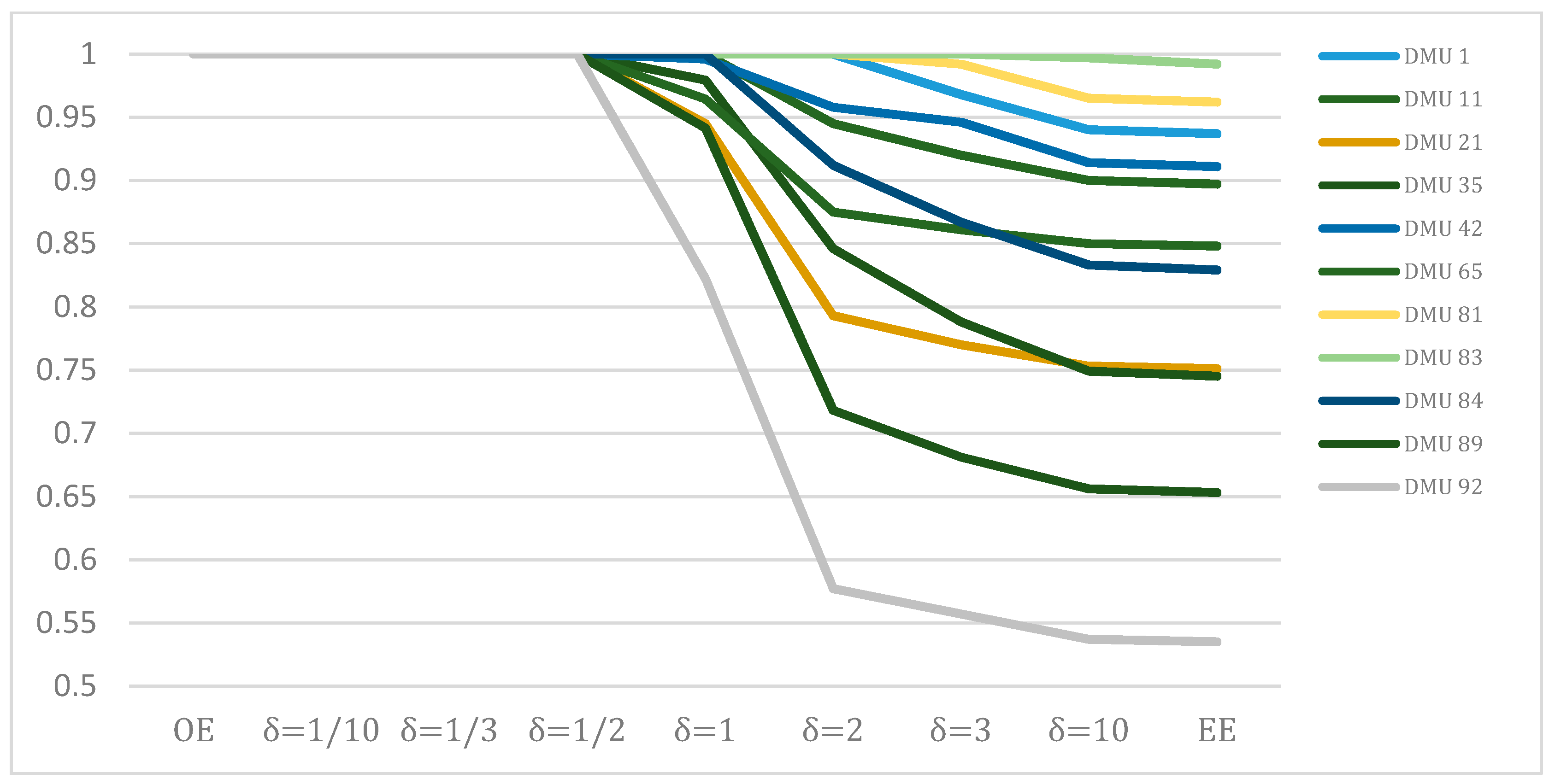
As shown in Figure 2, 11 DMUs (DMU 1, 11, 21, 35, 42, 65, 81, 83, 84, 89, 92) are operationally efficient but environmentally inefficient. Under Model (6) with δ = 1, all these DMUs are eco-efficient. However, the proposed method cannot carry out such a result because the environmental stringency is not identified. Therefore, in order to simluate the proposed method, we tried to derive the eco-effiency by changing the degree of environmental stringency. Figure 2 presents the changes of efficiency scores of 11 operationally efficient DMUs by changing δ from 1/10 to 10. From the results, we conclude that these 11 DMUs are eco-efficient when the operational concern is at least two times more important than the environmental concern. However, eco-efficiency scores are decreased as δ increases. In other words, eco-efficient DMUs in certain environments may not be eco-inefficient in other environments.
Figure 3 illustrates the efficiency changes of 29 DMUs, which are environmentally efficient but operationally inefficient. These 29 DMUs are regarded as being eco-efficient under Model (6) with δ = 1. However, the proposed model recognizes eco-efficient DMUs according to the environmental stringencty parameter. The simulation results show that all 29 DMUs are eco-efficient only when δ ≥ 2. The changes of the eco-efficiency of 29 DMUs are presented in Figure 3.
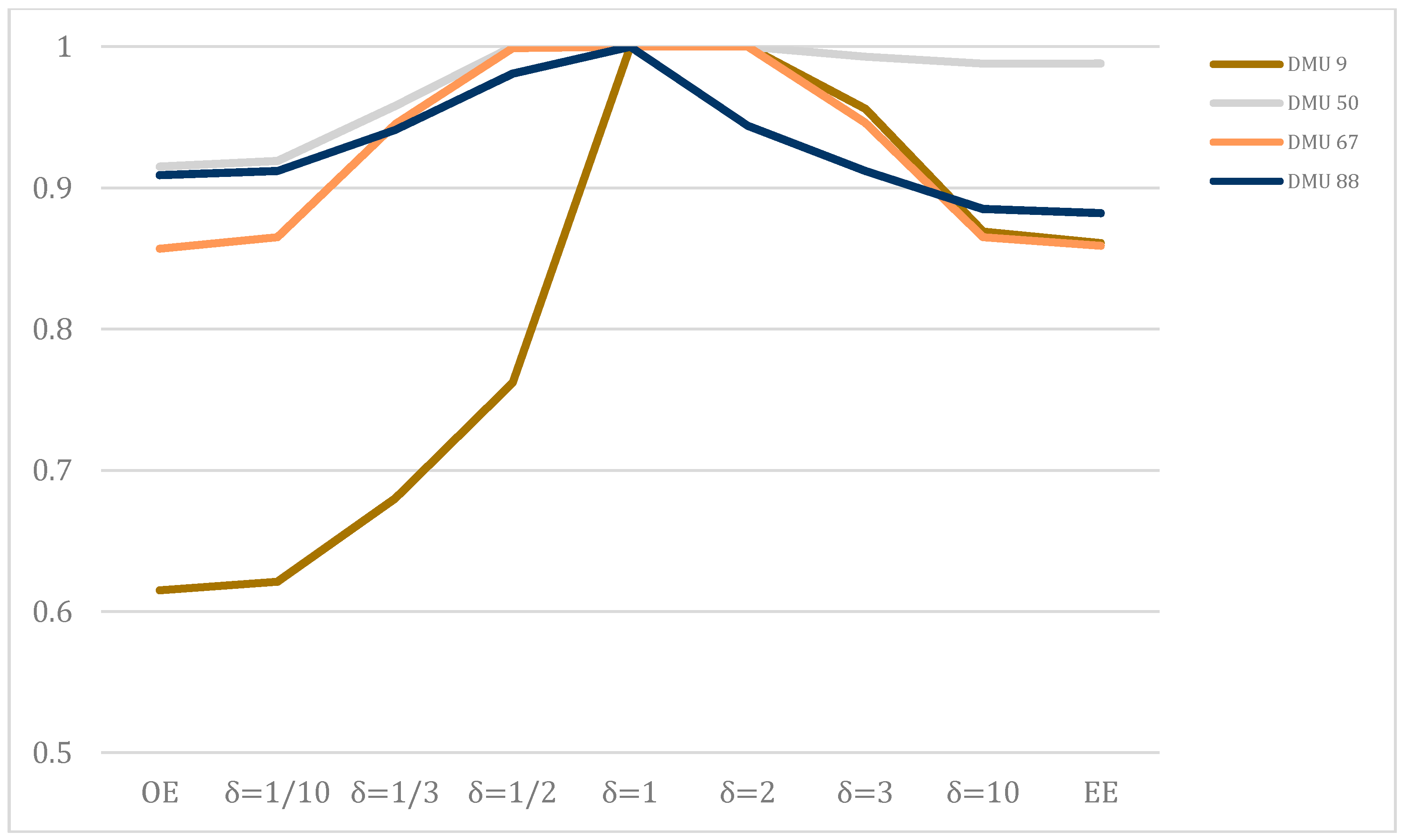
Again, we highlight that five DMUs are eco-efficient regardless of the environmental stringency. Now, in order to evaluate DMUs under the specified business conditions, we assume that the decision maker specifies the value of the stringency parameter. Assume δ equals one. Then 35 DMUs are eco-efficient. Among them, 26 DMUs are either operationally efficient or environmentally efficient. However, there are four DMUs (DMU 9, 50, 67, 88), as shown in Figure 4, which are neither operationally efficient nor environmental efficiency but are eco-efficient.
Additionally, the eco-efficiency scores of some DMUs are not skewed towards either operations-oriented situations or environment-oriented situations. For example, DMU 9, 50, 67, and 88 are eco-efficient on the condition that equal importance is given to operational and environmental concerns. However, we should note that the scores of operational efficiency and/or environmental efficiency are not equal to 1. This result explains that some DMUs can be evaluated as being eco-efficient under a certain condition, even if they are not operationally efficient or environmentally efficient.
4. Conclusions
In this paper, we proposed a more concrete and flexible DEA method for evaluating eco-efficiency. By using the environmental stringency constraints, the proposed model allows users to evaluate DMUs’ performance in accordance with their business conditions. We analyzed a case example to present the results by varying the value of the stringency parameter. Also, the results were compared with the results from Model B in [6,20].
The main contributions of this study are three-fold. Firstly, the proposed model provides the flexibility, as required by the pollution-intensity of industry, in that it allows the decision maker to appropriately evaluate a DMU’s eco-efficiency depending on the business environment. This approach overcomes the disadvantage in the earlier studies, which provide eco-efficiency evaluation models without considering environmental stringency. Different environmental stringencies can successively be incorporated in DEA. Through the use of selective parametric restrictions, DEA can flexibly be applied to the eco-efficiency evaluation problem. Secondly, the proposed model provides clarification or a link between operational and environmental efficiency in a different way from previous eco-efficiency research. In the previous studies, a particular DMU is treated as being eco-efficient if it is either operationally or environmentally efficient. In other words, eco-efficiency is derived by picking a more favorable score between operational efficiency and environmental efficiency. However, the proposed method shows that this property cannot be applied when the environmental stringency is considered. Thirdly, the proposed method enhances the discriminant power. This contribution may seem relatively minor, but it is worth noticing that it can generate a reasonable number of efficient DMUs and produce more realistic results in real-world applications because unconstrained weights on its inputs and outputs are usually unacceptable [41].
Some of the further research opportunities are as follows. First, this study examines eco-efficiency by decomposing inputs into operational and environmental inputs. However, both undesirable outputs and undesirable inputs are considered as environmental inputs in the illustrative example, although environmental inputs are defined as undesirable outputs in the proposed model. Therefore, a technique for treating these two factors separately will be helpful for the input-output context. Second, the role of the stringency parameter described in the Section 2.4 provides some other ideas for future studies, particularly including possible extensions of our method to situations where equal importance between operational and environmental aspects exists. Finally, we can expect that much further improvement by a more detailed case study will enhance the practical use of DEA for eco-efficiency evaluation.
However, there are some limitations to the proposed model. First, the major limitation is the process of eco-efficiency approximation by taking an average of two scores when both operational and environmental concerns are equally important. Since incorporating equal importance between operational and environmental concerns is unrealistic when it applied to the evaluation model, it requires convincing ways of systematical improvement on a theoretical basis. Second, the proposed method only considers the evaluation problem, where all DMUs follow the same environmental stringency. Therefore, one should adopt a different approach if several DMUs belong to different business environments. This limitation also provides opportunities for further studies. The last limitation is the non-statistical property of DEA. Since efficiency scores are obtained by deterministic computation based on the data without statistical assumptions, the results are very sensitive to the data. This inherent weakness of DEA made it difficult to interpret the statistical reliability of the results. However, it is expected that statistical techniques such as bootstrapping can be better incorporated into a DEA-based eco-efficiency study.
Acknowledgments
This work was supported by the Ministry of Education of the Republic of Korea and the National Research Foundation of Korea (NRF-2015S1A5B8046893).
Author Contributions
Pyoungsoo Lee conceived, designed, and performed the numerical analysis and wrote and revised the paper. You-Jin Park supervised the whole process and revised the paper.
Conflicts of Interest
The authors declare no conflict of interest.
Abbreviations
The following abbreviations are used in this manuscript:
| DEA | Data Envelopment Analysis | xij | amount of operational input i for DMU j |
| DMU | Decision Making Unit | zkj | amount of environmental input k for DMU j |
| LCI | Life Cycle Inventory | yrj | amount of output r for DMU j |
| MOLP | Multiple Objective Linear Programming | vi | non-negative weight for operational inputs i |
| CRS | Constant Return to Scale | wk | non-negative weight for environmental input k |
| ARII | Type II Assurance Region | ur | non-negative weight for output r |
| FYM | Farmyard Manure | δ | degree of environmental stringency |
| OE | Operational Efficiency | ||
| EE | Environmental Efficiency |
References
- Schaltegger, S.; Sturm, A. Ökologische Rationalität: Ansatzpunkte Zur ausgestaltung von ökologieorientierten Managementinstrumenten. Die Unternehm. 1990, 44, 273–290. [Google Scholar]
- DeSimone, L.D.; Popoff, F. Eco-efficiency: The Business Link to Sustainable Development; MIT Press: Cambridge, MA, USA, 2000. [Google Scholar]
- Charnes, A.; Cooper, W.W.; Rhodes, E. Measuring the efficiency of decision making units. Eur. J. Oper. Res. 1978, 2, 429–444. [Google Scholar] [CrossRef]
- Bevilacqua, M.; Braglia, M. Environmental efficiency analysis for ENI oil refineries. J. Clean. Prod. 2002, 10, 85–92. [Google Scholar] [CrossRef]
- Dyckhoff, H.; Allen, K. Measuring ecological efficiency with data envelopment analysis (DEA). Eur. J. Oper. Res. 2001, 132, 312–325. [Google Scholar] [CrossRef]
- Korhonen, P.J.; Luptacik, M. Eco-efficiency analysis of power plants: An extension of data envelopment analysis. Eur. J. Oper. Res. 2004, 154, 437–446. [Google Scholar] [CrossRef]
- Liang, L.; Wu, D.; Hua, Z. MES-DEA modelling for analysing anti-industrial pollution efficiency and its application in Anhui province of China. Int. J. Glob. Energy Issues 2004, 22, 88–98. [Google Scholar] [CrossRef]
- Mahdiloo, M.; Saen, R.F.; Lee, K.H. Technical, environmental and eco-efficiency measurement for supplier selection: An extension and application of data envelopment analysis. Int. J. Prod. Econ. 2015, 168, 279–289. [Google Scholar] [CrossRef]
- Murty, M.; Kumar, S.; Paul, M. Environmental regulation, productive efficiency and cost of pollution abatement: A case study of the sugar industry in India. J. Environ. Manag. 2006, 79, 1–9. [Google Scholar] [CrossRef] [PubMed]
- Pasurka, C.A. Decomposing electric power plant emissions within a joint production framework. Energy Econ. 2006, 28, 26–43. [Google Scholar] [CrossRef]
- Picazo-Tadeo, A.J.; Reig-Martinez, E.; Hernandez-Sancho, F. Directional distance functions and environmental regulation. Resour. Energy Econ. 2005, 27, 131–142. [Google Scholar] [CrossRef]
- Ramanathan, R. Combining indicators of energy consumption and CO2 emissions: A cross-country comparison. Int. J. Glob. Energy Issues 2002, 17, 214–227. [Google Scholar] [CrossRef]
- Song, M.; Zhang, L.; An, Q.; Wang, Z.; Li, Z. Statistical analysis and combination forecasting of environmental efficiency and its influential factors since China entered the WTO: 2002–2010–2012. J. Clean. Prod. 2013, 42, 42–51. [Google Scholar] [CrossRef]
- Sueyoshi, T.; Goto, M.; Ueno, T. Performance analysis of US coal-fired power plants by measuring three DEA efficiencies. Energy Policy 2010, 38, 1675–1688. [Google Scholar] [CrossRef]
- Triantis, K.; Otis, P. Dominance-based measurement of productive and environmental performance for manufacturing. Eur. J. Oper. Res. 2004, 154, 447–464. [Google Scholar] [CrossRef]
- Watanabe, M.; Tanaka, K. Efficiency analysis of Chinese industry: A directional distance function approach. Energy Policy 2007, 35, 6323–6331. [Google Scholar] [CrossRef]
- Wu, J.; An, Q.; Yao, X.; Wang, B. Environmental efficiency evaluation of industry in China based on a new fixed sum undesirable output data envelopment analysis. J. Clean. Prod. 2014, 74, 96–104. [Google Scholar] [CrossRef]
- Yang, H.; Pollitt, M. Incorporating both undesirable outputs and uncontrollable variables into DEA: The performance of Chinese coal-fired power plants. Eur. J. Oper. Res. 2009, 197, 1095–1105. [Google Scholar] [CrossRef]
- Zaim, O. Measuring environmental performance of state manufacturing through changes in pollution intensities: A DEA framework. Ecol. Econom. 2004, 48, 37–47. [Google Scholar] [CrossRef]
- Zhang, B.; Bi, J.; Fan, Z.; Yuan, Z.; Ge, J. Eco-efficiency analysis of industrial system in China: A data envelopment analysis approach. Ecol. Econom. 2008, 68, 306–316. [Google Scholar] [CrossRef]
- Zhou, P.; Ang, B.W. Linear programming models for measuring economy-wide energy efficiency performance. Energy Policy 2008, 36, 2911–2916. [Google Scholar] [CrossRef]
- Zhou, P.; Ang, B.W.; Poh, K.L. Measuring environmental performance under different environmental DEA technologies. Energy Econom. 2008, 30, 1–14. [Google Scholar] [CrossRef]
- Färe, R.; Grosskopf, S.; Lovell, C.K.; Pasurka, C. Multilateral productivity comparisons when some outputs are undesirable: A nonparametric approach. Rev. Econ. Stat. 1989, 71, 90–98. [Google Scholar] [CrossRef]
- Färe, R.; Grosskopf, S. Modeling undesirable factors in efficiency evaluation: Comment. Eur. J. Oper. Res. 2004, 157, 242–245. [Google Scholar] [CrossRef]
- Seiford, L.M.; Zhu, J. Modeling undesirable factors in efficiency evaluation. Eur. J. Oper. Res. 2002, 142, 16–20. [Google Scholar] [CrossRef]
- Liu, W.; Meng, W.; Li, X.; Zhang, D. DEA models with undesirable inputs and outputs. Ann. Oper. Res. 2010, 173, 177–194. [Google Scholar] [CrossRef]
- Pang, J.; Chen, X.; Zhang, Z.; Li, H. Measuring Eco-Efficiency of Agriculture in China. Sustainability 2016, 8, 398. [Google Scholar] [CrossRef]
- Pelletier, N.; Arsenault, N.; Tyedmers, P. Scenario modeling potential eco-efficiency gains from a transition to organic agriculture: Life cycle perspectives on Canadian canola, corn, soy, and wheat production. Environ. Manag. 2008, 42, 989–1001. [Google Scholar] [CrossRef] [PubMed]
- Mohammadi, A.; Rafiee, S.; Jafari, A.; Dalgaard, T.; Knudsen, M.T.; Keyhani, A.; Mousavi-Avval, S.H.; Hermansen, J.E. Potential greenhouse gas emission reductions in soybean farming: A combined use of life cycle assessment and data envelopment analysis. J. Clean. Prod. 2013, 54, 89–100. [Google Scholar] [CrossRef]
- Masuda, K. Measuring eco-efficiency of wheat production in Japan: A combined application of life cycle assessment and data envelopment analysis. J. Clean. Prod. 2016, 126, 373–381. [Google Scholar] [CrossRef]
- Picazo-Tadeo, A.J.; Gomez-Limon, J.A.; Reig-Martinez, E. Assessing farming eco-efficiency: A data envelopment analysis approach. J. Environ. Manag. 2011, 92, 1154–1164. [Google Scholar] [CrossRef] [PubMed]
- Li, J.C.; Li, J.Y.; Zheng, F.T. Unified efficiency measurement of electric power supply companies in China. Sustainability 2014, 6, 779–793. [Google Scholar] [CrossRef]
- Song, X.; Hao, Y.; Zhu, X. Analysis of the environmental efficiency of the Chinese transportation sector using an undesirable output slacks-based measure data envelopment analysis model. Sustainability 2015, 7, 9187–9206. [Google Scholar] [CrossRef]
- Hu, J.-L.; Kao, C.-H. Efficient energy-saving targets for APEC economies. Energy Policy 2007, 35, 373–382. [Google Scholar] [CrossRef]
- Hu, J.-L.; Wang, S.-C. Total-factor energy efficiency of regions in China. Energy Policy 2006, 34, 3206–3217. [Google Scholar] [CrossRef]
- Ramanathan, R. A holistic approach to compare energy efficiencies of different transport modes. Energy Policy 2000, 28, 743–747. [Google Scholar] [CrossRef]
- Charnes, A.; Cooper, W.W. Programming with linear fractional functionals. Naval Res. Logist. Q. 1962, 9, 181–186. [Google Scholar] [CrossRef]
- Golany, B.; Roll, Y. An application procedure for DEA. Omega 1989, 17, 237–250. [Google Scholar] [CrossRef]
- Cook, W.D.; Tone, K.; Zhu, J. Data envelopment analysis: Prior to choosing a model. Omega 2014, 44, 1–4. [Google Scholar] [CrossRef]
- Dyson, R.G.; Thanassoulis, E. Reducing weight flexibility in data envelopment analysis. J. Oper. Res. Soc. 1988, 39, 563–576. [Google Scholar] [CrossRef]
- Roll, Y.; Golany, B. Alternate methods of treating factor weights in DEA. Omega 1993, 21, 99–109. [Google Scholar] [CrossRef]
Figure 1.
The conceptual framework.
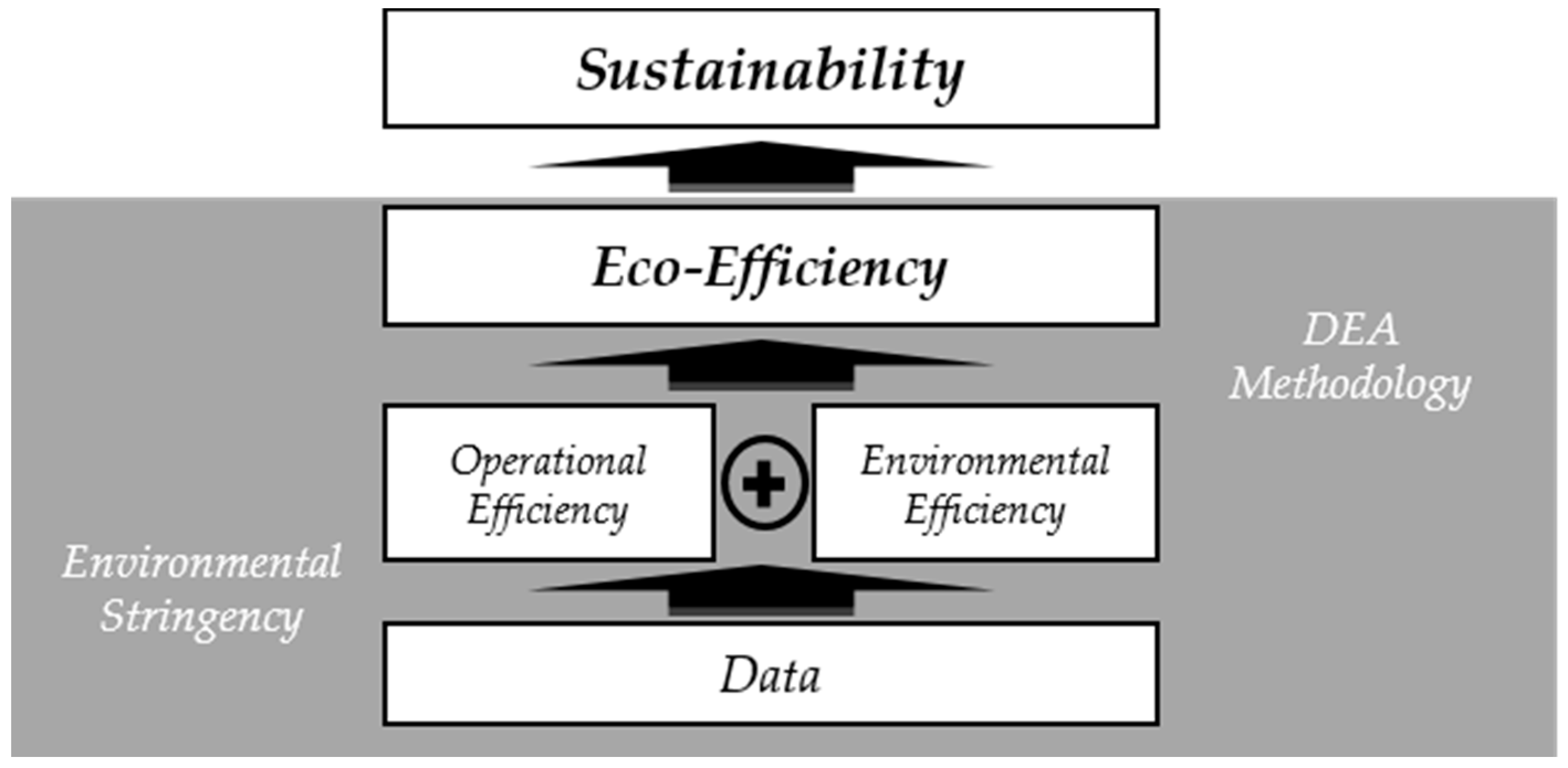
Figure 2.
Changes of operationally efficient DMUs.

Figure 3.
Changes of environmentally efficient DMUs.
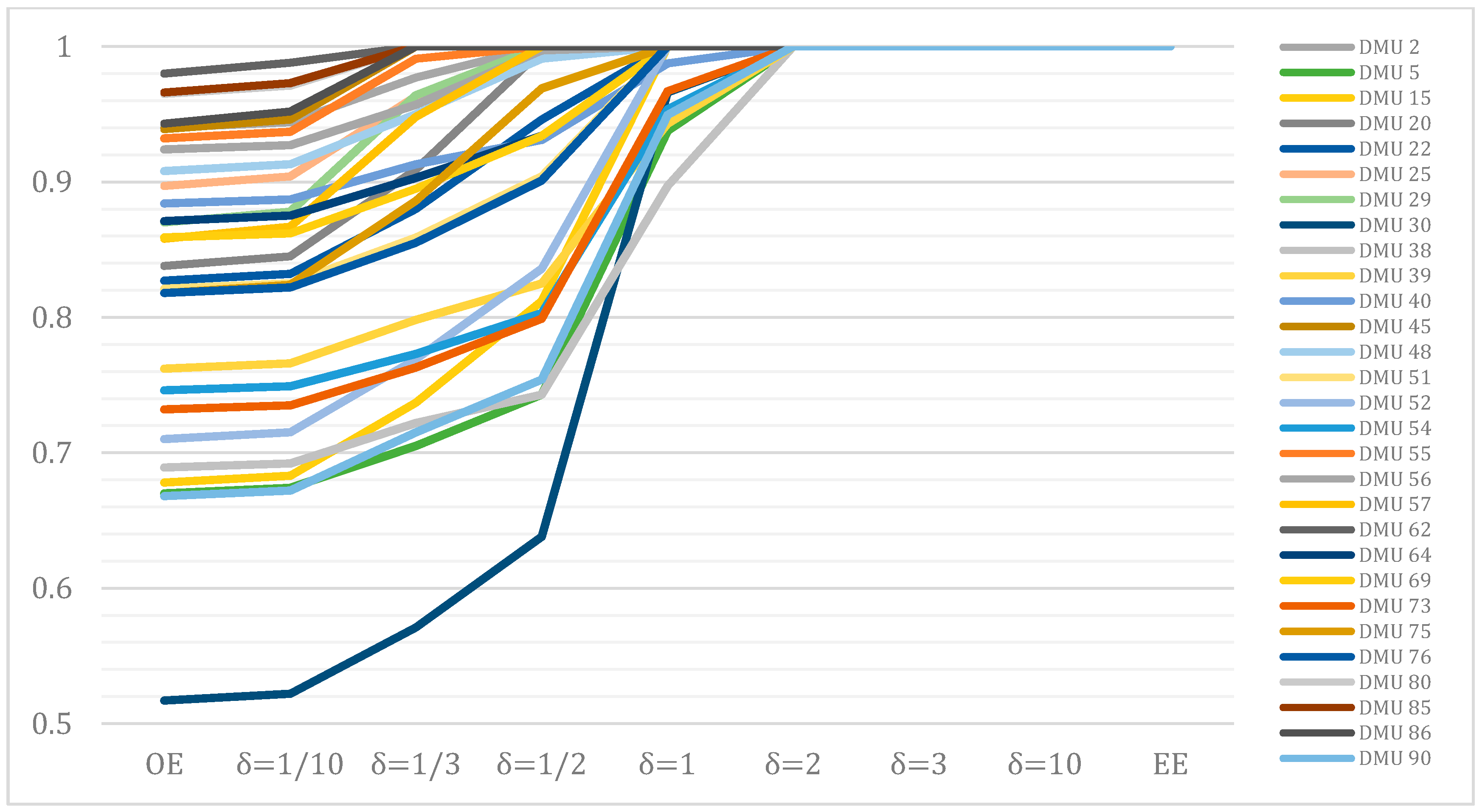
Figure 4.
Efficiency changes of DMU 9, 50, 67, and 88.


Table 1.
Input decomposition.
| Operational Inputs | Traditional Inputs | Labor (h) |
| Machinery (h) | ||
| Water (m3) | ||
| Seed (kg) | ||
| Energy | Diesel (L) | |
| Electricity (kWh) | ||
| Environmental Inputs | Chemicals | Herbicides (kg) |
| Insecticides (kg) | ||
| K2O (kg) | ||
| Fertilizers | Urea (kg) | |
| P2O5 (kg) | ||
| FYM (kg) | ||
| Undesirable Outputs | CH4 (kg) | |
| (direct gas emission) | N2O (kg) |
Table 2.
Data set for the analysis.
| DMU | Labor (h) | Machinery (h) | Water (m3) | Diesel (L) | Electricity (kWh) | Seed (kg) | Herbicides (kg) | Insecticides (kg) | Urea (kg) | P2O5 (kg) | K2O (kg) | FYM (kg) | CH4 (kg) | N2O (kg) | Soybean (kg) | Straw (kg) |
|---|---|---|---|---|---|---|---|---|---|---|---|---|---|---|---|---|
| 1 | 169 | 16 | 2016 | 70 | 0 | 60 | 4 | 1.5 | 110 | 46 | 0 | 0 | 9.3 | 3.2 | 3500 | 4312 |
| 2 | 142 | 15 | 2150 | 65 | 0 | 60 | 3 | 0.5 | 55 | 23 | 0 | 2500 | 8.4 | 3.1 | 3000 | 3889 |
| 3 | 197 | 22 | 3360 | 88 | 1953 | 70 | 2 | 1 | 96 | 69 | 0 | 2500 | 8.4 | 3.2 | 3000 | 3889 |
| 4 | 254 | 35 | 2722 | 122 | 1286 | 70 | 3 | 2 | 110 | 46 | 0 | 7500 | 9.5 | 3.4 | 3600 | 4397 |
| 5 | 138 | 32 | 2464 | 111 | 1432 | 100 | 2 | 2.5 | 78 | 23 | 0 | 2222 | 0 | 3.2 | 3000 | 3889 |
| 6 | 152 | 28 | 2419 | 98 | 0 | 60 | 3 | 2 | 110 | 46 | 0 | 2000 | 0 | 3.7 | 3150 | 4016 |
| 7 | 148 | 28 | 2419 | 109 | 703 | 60 | 3 | 3 | 110 | 46 | 0 | 563 | 0 | 3.2 | 4150 | 4862 |
| 8 | 213 | 27 | 4838 | 109 | 1406 | 100 | 1 | 2 | 137 | 115 | 0 | 1250 | 9.3 | 3.3 | 3500 | 4312 |
| 9 | 159 | 18 | 2822 | 76 | 0 | 80 | 0 | 2 | 76 | 46 | 0 | 0 | 7.1 | 3.1 | 2300 | 3296 |
| 10 | 137 | 28 | 2822 | 96 | 0 | 70 | 3 | 3.5 | 76 | 46 | 0 | 0 | 0 | 3.4 | 2300 | 3296 |
| 11 | 272 | 26 | 2016 | 105 | 0 | 63 | 3 | 2 | 103 | 115 | 0 | 750 | 9.3 | 3.2 | 3500 | 4312 |
| 12 | 185 | 31 | 2419 | 126 | 1406 | 60 | 3 | 4.5 | 82 | 92 | 0 | 1500 | 0 | 3.6 | 3400 | 4227 |
| 13 | 228 | 35 | 1344 | 119 | 781 | 80 | 3 | 5 | 82 | 92 | 0 | 7500 | 8.4 | 3.4 | 3000 | 3889 |
| 14 | 264 | 22 | 1890 | 91 | 0 | 100 | 3 | 2 | 100 | 72 | 0 | 0 | 7.1 | 3.2 | 2315 | 3309 |
| 15 | 200 | 45 | 4032 | 150 | 1758 | 80 | 0 | 1.5 | 92 | 0 | 0 | 16,667 | 9.8 | 3.6 | 3750 | 4524 |
| 16 | 289 | 32 | 3528 | 115 | 2179 | 75 | 3 | 1.5 | 114 | 115 | 0 | 7500 | 0 | 3.4 | 3250 | 4100 |
| 17 | 282 | 35 | 3024 | 130 | 1758 | 60 | 3 | 2.5 | 105 | 92 | 0 | 4500 | 0 | 3.3 | 3500 | 4312 |
| 18 | 209 | 24 | 2621 | 83 | 1524 | 80 | 3 | 1 | 92 | 0 | 0 | 6000 | 7.7 | 3.3 | 2600 | 3550 |
| 19 | 268 | 33 | 7258 | 119 | 2901 | 80 | 3 | 8 | 92 | 0 | 0 | 12,500 | 8.4 | 3.5 | 3000 | 3889 |
| 20 | 210 | 55 | 3024 | 168 | 1538 | 60 | 0 | 1 | 64 | 46 | 0 | 10,000 | 9.3 | 3.4 | 35,007 | 4312 |
| 21 | 139 | 27 | 1260 | 108 | 732 | 60 | 3 | 4.5 | 114 | 115 | 0 | 9375 | 0 | 3.9 | 3500 | 4312 |
| 22 | 179 | 23 | 4536 | 109 | 1154 | 80 | 5 | 0.5 | 69 | 0 | 0 | 4000 | 0 | 3.8 | 4000 | 4735 |
| 23 | 200 | 40 | 2822 | 131 | 820 | 70 | 3 | 3.5 | 114 | 115 | 0 | 1111 | 8.6 | 3.2 | 3115 | 3986 |
| 24 | 245 | 29 | 2016 | 106 | 1172 | 80 | 3 | 1.5 | 87 | 46 | 0 | 3750 | 9.3 | 3.3 | 3500 | 4312 |
| 25 | 222 | 31 | 3226 | 93 | 1289 | 80 | 3 | 8 | 0 | 0 | 0 | 11,000 | 10.6 | 3.3 | 4200 | 4904 |
| 26 | 263 | 54 | 5443 | 175 | 2175 | 70 | 3 | 3.5 | 92 | 0 | 0 | 12,500 | 8.6 | 3.5 | 3100 | 3974 |
| 27 | 285 | 64 | 5443 | 203 | 2175 | 70 | 3 | 2.5 | 92 | 0 | 0 | 25,000 | 8.4 | 3.9 | 3000 | 3889 |
| 28 | 124 | 17 | 2419 | 69 | 0 | 55 | 3 | 0.5 | 78 | 23 | 25 | 0 | 0 | 3.5 | 3200 | 4058 |
| 29 | 215 | 15 | 5645 | 88 | 3282 | 70 | 0 | 1 | 87 | 46 | 0 | 0 | 9.3 | 3.1 | 3500 | 4312 |
| 30 | 134 | 14 | 4838 | 76 | 1406 | 70 | 0 | 1.5 | 69 | 0 | 0 | 0 | 6.6 | 3.1 | 2000 | 3043 |
| 31 | 137 | 17 | 2016 | 64 | 1318 | 60 | 3 | 3 | 78 | 23 | 0 | 833 | 0 | 3.1 | 3300 | 4143 |
| 32 | 201 | 17 | 3024 | 68 | 879 | 60 | 3 | 0.5 | 110 | 46 | 0 | 0 | 0 | 3.2 | 3600 | 4397 |
| 33 | 159 | 38 | 3528 | 128 | 2051 | 70 | 3 | 2.5 | 110 | 46 | 0 | 7500 | 9.3 | 3.4 | 3500 | 4312 |
| 34 | 269 | 50 | 2016 | 160 | 732 | 60 | 3 | 5.5 | 64 | 46 | 0 | 0 | 10.6 | 3.1 | 4200 | 4904 |
| 35 | 223 | 10 | 4838 | 65 | 2813 | 60 | 3 | 4.5 | 64 | 46 | 0 | 1500 | 8.4 | 3.1 | 3000 | 3889 |
| 36 | 145 | 24 | 3360 | 101 | 2075 | 60 | 0 | 3 | 64 | 46 | 0 | 0 | 7.5 | 3.1 | 2500 | 3466 |
| 37 | 176 | 29 | 4032 | 108 | 1172 | 70 | 3 | 2 | 64 | 46 | 0 | 2083 | 0 | 3.6 | 3500 | 4312 |
| 38 | 183 | 29 | 3629 | 100 | 1450 | 60 | 3 | 10.6 | 48 | 35 | 0 | 208 | 0 | 3.1 | 2800 | 3720 |
| 39 | 167 | 23 | 6048 | 93 | 3076 | 60 | 3 | 2.5 | 50 | 69 | 0 | 0 | 0 | 3.5 | 3000 | 3889 |
| 40 | 238 | 26 | 4032 | 95 | 879 | 55 | 3 | 2.5 | 64 | 46 | 0 | 0 | 9 | 3.1 | 3330 | 4168 |
| 41 | 290 | 34 | 6048 | 117 | 3516 | 90 | 3 | 6 | 197 | 92 | 0 | 0 | 9.3 | 3.4 | 3500 | 4312 |
| 42 | 206 | 24 | 3528 | 93 | 2051 | 60 | 3 | 5 | 128 | 92 | 0 | 3000 | 10.2 | 3.3 | 4000 | 4735 |
| 43 | 350 | 21 | 4032 | 120 | 1538 | 60 | 4 | 5 | 159 | 92 | 0 | 3000 | 9.1 | 3.4 | 3400 | 4227 |
| 44 | 133 | 31 | 3024 | 100 | 1154 | 75 | 3 | 6.5 | 96 | 69 | 0 | 0 | 9.3 | 3.2 | 3500 | 4312 |
| 45 | 169 | 25 | 3528 | 92 | 1025 | 70 | 3 | 3.5 | 0 | 0 | 0 | 6250 | 0 | 3.7 | 4000 | 4735 |
| 46 | 157 | 34 | 2822 | 108 | 820 | 70 | 3 | 3 | 110 | 46 | 0 | 3750 | 8 | 3.3 | 2800 | 3720 |
| 47 | 239 | 35 | 2822 | 120 | 1641 | 70 | 3 | 3.6 | 156 | 46 | 0 | 15,000 | 0 | 4.3 | 4000 | 4735 |
| 48 | 170 | 21 | 3360 | 89 | 855 | 60 | 3 | 1.5 | 115 | 0 | 150 | 0 | 9.3 | 3.2 | 3500 | 4312 |
| 49 | 220 | 50 | 3110 | 146 | 1582 | 80 | 3 | 4 | 135 | 81 | 13 | 10,000 | 9.3 | 3.5 | 3500 | 4312 |
| 50 | 277 | 29 | 4838 | 117 | 2813 | 60 | 1.25 | 4.5 | 110 | 46 | 0 | 0 | 9.9 | 3.2 | 3800 | 4566 |
| 51 | 186 | 48 | 2952 | 165 | 1791 | 65 | 1.5 | 3 | 92 | 0 | 0 | 21,429 | 0 | 4.3 | 3700 | 4481 |
| 52 | 189 | 20 | 2688 | 81 | 781 | 60 | 0 | 1.5 | 64 | 46 | 0 | 0 | 7.8 | 3.1 | 2666 | 3606 |
| 53 | 104 | 35 | 4838 | 124 | 2110 | 60 | 3 | 3 | 83 | 23 | 0 | 12,000 | 7.7 | 3.5 | 2600 | 3550 |
| 54 | 170 | 19 | 2520 | 75 | 1465 | 60 | 3 | 2 | 92 | 0 | 0 | 0 | 7.9 | 3.2 | 2700 | 3635 |
| 55 | 112 | 20 | 3226 | 101 | 2110 | 70 | 2 | 3 | 92 | 0 | 125 | 0 | 9.1 | 3.2 | 3400 | 4227 |
| 56 | 144 | 25 | 2112 | 106 | 1074 | 60 | 3.5 | 0.3 | 110 | 46 | 0 | 1500 | 0 | 3.7 | 3570 | 4371 |
| 57 | 179 | 15 | 3024 | 86 | 1978 | 60 | 0 | 1.5 | 92 | 0 | 100 | 0 | 8.4 | 3.2 | 3000 | 3889 |
| 58 | 215 | 30 | 3024 | 109 | 769 | 55 | 3 | 3 | 123 | 138 | 0 | 22,500 | 0 | 3.9 | 3500 | 4312 |
| 59 | 146 | 34 | 3629 | 134 | 1846 | 70 | 3 | 2.5 | 87 | 46 | 0 | 15,000 | 0 | 4.1 | 3800 | 4566 |
| 60 | 162 | 40 | 4657 | 147 | 2369 | 70 | 3 | 2.5 | 87 | 46 | 0 | 15,000 | 9.3 | 3.6 | 3500 | 4312 |
| 61 | 245 | 34 | 3528 | 119 | 1410 | 70 | 3 | 3 | 92 | 0 | 100 | 10,000 | 8.4 | 3.4 | 3000 | 3889 |
| 62 | 196 | 9 | 2016 | 61 | 513 | 100 | 3 | 2.5 | 32 | 23 | 0 | 417 | 0 | 3.4 | 2500 | 3466 |
| 63 | 187 | 19 | 2957 | 79 | 1934 | 70 | 2 | 2.5 | 137 | 115 | 0 | 0 | 8 | 3.3 | 2800 | 3720 |
| 64 | 163 | 21 | 2880 | 88 | 1465 | 70 | 3 | 3 | 115 | 0 | 50 | 2500 | 9.4 | 3.3 | 3570 | 4371 |
| 65 | 243 | 21 | 3024 | 86 | 824 | 55 | 3 | 3 | 123 | 138 | 0 | 5000 | 9.7 | 3.4 | 3700 | 4481 |
| 66 | 196 | 22 | 3326 | 103 | 2175 | 70 | 3 | 2.5 | 137 | 115 | 0 | 0 | 8 | 3.3 | 2800 | 3720 |
| 67 | 178 | 26 | 2150 | 100 | 0 | 60 | 3.5 | 0.3 | 110 | 46 | 0 | 1500 | 0 | 3.6 | 3000 | 3889 |
| 68 | 214 | 33 | 2688 | 132 | 1367 | 70 | 3.5 | 3 | 110 | 46 | 0 | 7500 | 0 | 3.9 | 3500 | 4312 |
| 69 | 169 | 27 | 2520 | 92 | 1282 | 70 | 3.5 | 0.5 | 92 | 0 | 50 | 7500 | 0 | 3.9 | 3600 | 4397 |
| 70 | 208 | 28 | 2464 | 104 | 1432 | 70 | 3 | 3 | 123 | 138 | 0 | 20,000 | 8 | 3.8 | 2800 | 3720 |
| 71 | 165 | 37 | 4032 | 124 | 1758 | 70 | 3 | 2 | 77 | 0 | 0 | 15,000 | 0 | 4 | 3500 | 4312 |
| 72 | 261 | 32 | 3528 | 124 | 2179 | 70 | 3 | 1.5 | 114 | 115 | 0 | 7500 | 0 | 3.8 | 2900 | 3804 |
| 73 | 283 | 38 | 3024 | 138 | 1758 | 70 | 3 | 1.5 | 69 | 0 | 100 | 5000 | 9.4 | 3.2 | 3550 | 4354 |
| 74 | 167 | 37 | 3276 | 136 | 1904 | 70 | 3 | 1 | 92 | 0 | 0 | 7500 | 7.7 | 3.4 | 2600 | 3550 |
| 75 | 211 | 31 | 2903 | 122 | 1477 | 60 | 0 | 1 | 46 | 0 | 50 | 10,000 | 9.1 | 3.3 | 3400 | 4227 |
| 76 | 155 | 36 | 3780 | 129 | 1030 | 70 | 3 | 2.5 | 69 | 0 | 0 | 10,000 | 0 | 3.4 | 3800 | 4566 |
| 77 | 154 | 30 | 2520 | 96 | 1007 | 70 | 3 | 2 | 110 | 46 | 0 | 7500 | 0 | 3.4 | 3300 | 4143 |
| 78 | 176 | 28 | 6451 | 119 | 2344 | 80 | 3 | 2.5 | 92 | 0 | 50 | 0 | 7.7 | 3.2 | 2600 | 3550 |
| 79 | 195 | 18 | 3629 | 89 | 1846 | 80 | 3 | 6 | 119 | 69 | 0 | 10,000 | 8.9 | 3.5 | 3300 | 4143 |
| 80 | 144 | 21 | 3226 | 93 | 1641 | 70 | 2 | 3 | 137 | 115 | 0 | 0 | 0 | 3.8 | 3900 | 4651 |
| 81 | 108 | 29 | 1613 | 98 | 820 | 60 | 3.5 | 1.5 | 64 | 46 | 0 | 7500 | 0 | 3.8 | 3700 | 4481 |
| 82 | 279 | 27 | 3360 | 116 | 916 | 90 | 4 | 4.5 | 160 | 115 | 0 | 15,000 | 8.9 | 3.7 | 3300 | 4143 |
| 83 | 309 | 12 | 2822 | 55 | 820 | 80 | 1 | 1 | 128 | 92 | 0 | 0 | 9.5 | 3.2 | 3600 | 4397 |
| 84 | 95 | 12 | 4704 | 66 | 0 | 60 | 3.5 | 2.5 | 87 | 46 | 50 | 10,000 | 0 | 3.4 | 3400 | 4227 |
| 85 | 141 | 25 | 2268 | 105 | 0 | 60 | 2 | 1.5 | 174 | 92 | 0 | 0 | 0 | 3.3 | 3200 | 4058 |
| 86 | 152 | 27 | 2100 | 103 | 0 | 60 | 0 | 2.5 | 91 | 115 | 0 | 12,500 | 0 | 3.9 | 3150 | 4016 |
| 87 | 127 | 19 | 2520 | 82 | 0 | 65 | 3 | 4.5 | 114 | 115 | 0 | 9375 | 8.5 | 3.5 | 3050 | 3931 |
| 88 | 121 | 21 | 2016 | 84 | 1172 | 60 | 3 | 2 | 46 | 0 | 0 | 10,000 | 0 | 3.8 | 3100 | 3974 |
| 89 | 213 | 6 | 2688 | 47 | 1074 | 70 | 2 | 1.5 | 105 | 92 | 0 | 0 | 0 | 3.2 | 2000 | 3043 |
| 90 | 171 | 17 | 4032 | 69 | 2344 | 70 | 3 | 1 | 92 | 0 | 0 | 0 | 0 | 3.5 | 2500 | 3466 |
| 91 | 192 | 18 | 6451 | 87 | 328 | 75 | 3 | 1 | 64 | 46 | 0 | 18,667 | 0 | 4 | 3000 | 3889 |
| 92 | 217 | 6 | 2688 | 48 | 1074 | 70 | 3 | 1.5 | 105 | 92 | 0 | 0 | 6.6 | 3.2 | 2000 | 3043 |
| 93 | 199 | 19 | 3629 | 72 | 2110 | 60 | 3 | 2 | 64 | 46 | 0 | 0 | 8.4 | 3.1 | 3000 | 3889 |
| 94 | 211 | 16 | 2520 | 58 | 1007 | 60 | 3 | 1.5 | 110 | 46 | 0 | 0 | 0 | 3.2 | 3200 | 4058 |
DMU: decision-making unit; FYM: farmyard manure.
Table 3.
Data envelopment analysis (DEA) results.
| DMU | Model (6) (δ = 1) | OE | δ = 1/10 | δ = 1/3 | δ = 1/2 | δ = 1 | δ = 2 | δ = 3 | δ = 10 | EE |
|---|---|---|---|---|---|---|---|---|---|---|
| 1 | 1 | 1 | 1 | 1 | 1 | 1 | 1 | 0.968 | 0.94 | 0.937 |
| 2 | 1 | 0.94 | 0.944 | 0.977 | 1 | 1 | 1 | 1 | 1 | 1 |
| 3 | 0.836 | 0.706 | 0.709 | 0.732 | 0.759 | 0.823 | 0.834 | 0.832 | 0.824 | 0.823 |
| 4 | 0.888 | 0.76 | 0.761 | 0.773 | 0.786 | 0.86 | 0.882 | 0.88 | 0.875 | 0.874 |
| 5 | 1 | 0.67 | 0.674 | 0.705 | 0.743 | 0.938 | 1 | 1 | 1 | 1 |
| 6 | 1 | 0.901 | 0.908 | 0.976 | 1 | 0.981 | 0.827 | 0.8 | 0.774 | 0.772 |
| 7 | 1 | 1 | 1 | 1 | 1 | 1 | 1 | 1 | 1 | 1 |
| 8 | 0.97 | 0.625 | 0.63 | 0.673 | 0.731 | 0.914 | 0.939 | 0.921 | 0.895 | 0.892 |
| 9 | 1 | 0.615 | 0.621 | 0.68 | 0.762 | 1 | 1 | 0.956 | 0.869 | 0.861 |
| 10 | 1 | 0.642 | 0.645 | 0.68 | 0.719 | 0.918 | 0.879 | 0.82 | 0.765 | 0.76 |
| 11 | 1 | 1 | 1 | 1 | 1 | 1 | 0.945 | 0.92 | 0.9 | 0.897 |
| 12 | 0.895 | 0.818 | 0.819 | 0.83 | 0.845 | 0.88 | 0.871 | 0.866 | 0.854 | 0.852 |
| 13 | 0.903 | 0.804 | 0.806 | 0.831 | 0.86 | 0.832 | 0.702 | 0.684 | 0.67 | 0.669 |
| 14 | 0.783 | 0.706 | 0.707 | 0.719 | 0.733 | 0.727 | 0.644 | 0.624 | 0.609 | 0.607 |
| 15 | 1 | 0.678 | 0.683 | 0.737 | 0.812 | 1 | 1 | 1 | 1 | 1 |
| 16 | 0.823 | 0.659 | 0.661 | 0.673 | 0.686 | 0.774 | 0.823 | 0.823 | 0.823 | 0.823 |
| 17 | 0.872 | 0.84 | 0.843 | 0.848 | 0.854 | 0.869 | 0.862 | 0.861 | 0.86 | 0.86 |
| 18 | 0.923 | 0.605 | 0.607 | 0.632 | 0.665 | 0.832 | 0.788 | 0.776 | 0.765 | 0.764 |
| 19 | 0.704 | 0.572 | 0.575 | 0.599 | 0.624 | 0.688 | 0.703 | 0.702 | 0.701 | 0.701 |
| 20 | 1 | 0.838 | 0.845 | 0.909 | 0.997 | 1 | 1 | 1 | 1 | 1 |
| 21 | 1 | 1 | 1 | 1 | 1 | 0.945 | 0.793 | 0.77 | 0.753 | 0.751 |
| 22 | 1 | 0.827 | 0.832 | 0.88 | 0.946 | 1 | 1 | 1 | 1 | 1 |
| 23 | 0.745 | 0.643 | 0.644 | 0.651 | 0.659 | 0.716 | 0.745 | 0.745 | 0.745 | 0.745 |
| 24 | 0.983 | 0.821 | 0.823 | 0.847 | 0.871 | 0.956 | 0.963 | 0.942 | 0.92 | 0.917 |
| 25 | 1 | 0.897 | 0.904 | 0.963 | 1 | 1 | 1 | 1 | 1 | 1 |
| 26 | 0.797 | 0.635 | 0.638 | 0.659 | 0.685 | 0.789 | 0.785 | 0.781 | 0.777 | 0.777 |
| 27 | 0.78 | 0.614 | 0.616 | 0.64 | 0.666 | 0.762 | 0.716 | 0.707 | 0.7 | 0.699 |
| 28 | 1 | 1 | 1 | 1 | 1 | 1 | 1 | 1 | 1 | 1 |
| 29 | 1 | 0.87 | 0.878 | 0.964 | 1 | 1 | 1 | 1 | 1 | 1 |
| 30 | 1 | 0.517 | 0.522 | 0.571 | 0.638 | 0.966 | 1 | 1 | 1 | 1 |
| 31 | 1 | 1 | 1 | 1 | 1 | 1 | 1 | 1 | 1 | 1 |
| 32 | 1 | 1 | 1 | 1 | 1 | 1 | 1 | 1 | 1 | 1 |
| 33 | 0.841 | 0.747 | 0.748 | 0.758 | 0.769 | 0.824 | 0.834 | 0.831 | 0.828 | 0.828 |
| 34 | 1 | 1 | 1 | 1 | 1 | 1 | 1 | 1 | 1 | 1 |
| 35 | 1 | 1 | 1 | 1 | 1 | 0.98 | 0.846 | 0.788 | 0.749 | 0.745 |
| 36 | 1 | 0.629 | 0.634 | 0.68 | 0.739 | 0.976 | 0.984 | 0.966 | 0.95 | 0.948 |
| 37 | 0.964 | 0.769 | 0.772 | 0.797 | 0.814 | 0.915 | 0.959 | 0.956 | 0.953 | 0.953 |
| 38 | 1 | 0.689 | 0.692 | 0.722 | 0.743 | 0.897 | 1 | 1 | 1 | 1 |
| 39 | 1 | 0.762 | 0.766 | 0.798 | 0.825 | 0.943 | 1 | 1 | 1 | 1 |
| 40 | 1 | 0.884 | 0.887 | 0.913 | 0.931 | 0.988 | 1 | 1 | 1 | 1 |
| 41 | 0.834 | 0.623 | 0.625 | 0.64 | 0.658 | 0.778 | 0.83 | 0.813 | 0.798 | 0.796 |
| 42 | 1 | 1 | 1 | 1 | 1 | 0.996 | 0.958 | 0.946 | 0.914 | 0.911 |
| 43 | 0.881 | 0.866 | 0.869 | 0.881 | 0.881 | 0.864 | 0.799 | 0.784 | 0.753 | 0.75 |
| 44 | 1 | 0.819 | 0.823 | 0.868 | 0.926 | 0.985 | 0.913 | 0.87 | 0.835 | 0.832 |
| 45 | 1 | 0.939 | 0.946 | 1 | 1 | 1 | 1 | 1 | 1 | 1 |
| 46 | 0.666 | 0.63 | 0.631 | 0.64 | 0.65 | 0.666 | 0.663 | 0.662 | 0.661 | 0.661 |
| 47 | 0.901 | 0.845 | 0.846 | 0.855 | 0.864 | 0.882 | 0.847 | 0.835 | 0.825 | 0.824 |
| 48 | 1 | 0.908 | 0.913 | 0.95 | 0.991 | 1 | 1 | 1 | 1 | 1 |
| 49 | 0.77 | 0.639 | 0.64 | 0.651 | 0.663 | 0.737 | 0.77 | 0.77 | 0.77 | 0.77 |
| 50 | 1 | 0.915 | 0.919 | 0.958 | 1 | 1 | 1 | 0.993 | 0.988 | 0.988 |
| 51 | 1 | 0.821 | 0.825 | 0.859 | 0.904 | 1 | 1 | 1 | 1 | 1 |
| 52 | 1 | 0.71 | 0.715 | 0.769 | 0.836 | 1 | 1 | 1 | 1 | 1 |
| 53 | 0.83 | 0.721 | 0.723 | 0.748 | 0.769 | 0.773 | 0.651 | 0.636 | 0.625 | 0.623 |
| 54 | 1 | 0.746 | 0.749 | 0.773 | 0.803 | 0.954 | 1 | 1 | 1 | 1 |
| 55 | 1 | 0.932 | 0.937 | 0.991 | 1 | 1 | 1 | 1 | 1 | 1 |
| 56 | 1 | 0.924 | 0.927 | 0.957 | 0.997 | 1 | 1 | 1 | 1 | 1 |
| 57 | 1 | 0.858 | 0.867 | 0.948 | 1 | 1 | 1 | 1 | 1 | 1 |
| 58 | 0.92 | 0.918 | 0.92 | 0.92 | 0.92 | 0.872 | 0.781 | 0.77 | 0.762 | 0.761 |
| 59 | 0.932 | 0.837 | 0.838 | 0.853 | 0.869 | 0.923 | 0.901 | 0.881 | 0.864 | 0.862 |
| 60 | 0.837 | 0.741 | 0.743 | 0.756 | 0.771 | 0.822 | 0.829 | 0.824 | 0.82 | 0.819 |
| 61 | 0.78 | 0.628 | 0.631 | 0.655 | 0.681 | 0.766 | 0.78 | 0.779 | 0.776 | 0.775 |
| 62 | 1 | 0.98 | 0.988 | 1 | 1 | 1 | 1 | 1 | 1 | 1 |
| 63 | 0.781 | 0.693 | 0.696 | 0.725 | 0.747 | 0.771 | 0.741 | 0.723 | 0.707 | 0.705 |
| 64 | 1 | 0.871 | 0.875 | 0.903 | 0.934 | 1 | 1 | 1 | 1 | 1 |
| 65 | 1 | 1 | 1 | 1 | 1 | 0.965 | 0.875 | 0.861 | 0.85 | 0.848 |
| 66 | 0.75 | 0.647 | 0.649 | 0.663 | 0.673 | 0.721 | 0.727 | 0.714 | 0.703 | 0.701 |
| 67 | 1 | 0.857 | 0.865 | 0.945 | 0.999 | 1 | 1 | 0.946 | 0.865 | 0.859 |
| 68 | 0.766 | 0.733 | 0.734 | 0.739 | 0.744 | 0.764 | 0.752 | 0.746 | 0.741 | 0.74 |
| 69 | 1 | 0.859 | 0.862 | 0.895 | 0.934 | 1 | 1 | 1 | 1 | 1 |
| 70 | 0.656 | 0.635 | 0.636 | 0.65 | 0.656 | 0.64 | 0.605 | 0.597 | 0.588 | 0.587 |
| 71 | 0.958 | 0.737 | 0.74 | 0.769 | 0.808 | 0.946 | 0.933 | 0.926 | 0.92 | 0.919 |
| 72 | 0.695 | 0.602 | 0.603 | 0.615 | 0.627 | 0.685 | 0.695 | 0.695 | 0.695 | 0.695 |
| 73 | 1 | 0.732 | 0.735 | 0.763 | 0.799 | 0.967 | 1 | 1 | 1 | 1 |
| 74 | 0.798 | 0.544 | 0.546 | 0.569 | 0.599 | 0.757 | 0.742 | 0.733 | 0.726 | 0.726 |
| 75 | 1 | 0.818 | 0.824 | 0.886 | 0.969 | 1 | 1 | 1 | 1 | 1 |
| 76 | 1 | 0.818 | 0.822 | 0.855 | 0.901 | 1 | 1 | 1 | 1 | 1 |
| 77 | 0.855 | 0.787 | 0.788 | 0.801 | 0.815 | 0.852 | 0.837 | 0.828 | 0.821 | 0.82 |
| 78 | 0.883 | 0.511 | 0.512 | 0.53 | 0.555 | 0.76 | 0.883 | 0.883 | 0.883 | 0.883 |
| 79 | 0.853 | 0.762 | 0.765 | 0.789 | 0.812 | 0.839 | 0.767 | 0.75 | 0.719 | 0.716 |
| 80 | 1 | 0.965 | 0.971 | 1 | 1 | 1 | 1 | 1 | 1 | 1 |
| 81 | 1 | 1 | 1 | 1 | 1 | 1 | 1 | 0.992 | 0.965 | 0.962 |
| 82 | 0.715 | 0.606 | 0.607 | 0.623 | 0.639 | 0.696 | 0.701 | 0.694 | 0.679 | 0.678 |
| 83 | 1 | 1 | 1 | 1 | 1 | 1 | 1 | 1 | 0.997 | 0.992 |
| 84 | 1 | 1 | 1 | 1 | 1 | 1 | 0.912 | 0.867 | 0.833 | 0.829 |
| 85 | 1 | 0.966 | 0.973 | 1 | 1 | 1 | 1 | 1 | 1 | 1 |
| 86 | 1 | 0.943 | 0.952 | 1 | 1 | 1 | 1 | 1 | 1 | 1 |
| 87 | 1 | 0.927 | 0.932 | 0.986 | 1 | 0.914 | 0.723 | 0.696 | 0.669 | 0.666 |
| 88 | 1 | 0.909 | 0.912 | 0.941 | 0.981 | 1 | 0.944 | 0.912 | 0.885 | 0.882 |
| 89 | 1 | 1 | 1 | 1 | 1 | 0.942 | 0.718 | 0.681 | 0.656 | 0.653 |
| 90 | 1 | 0.668 | 0.672 | 0.715 | 0.754 | 0.95 | 1 | 1 | 1 | 1 |
| 91 | 1 | 0.683 | 0.686 | 0.715 | 0.749 | 0.954 | 0.961 | 0.942 | 0.928 | 0.926 |
| 92 | 1 | 1 | 1 | 1 | 1 | 0.823 | 0.577 | 0.557 | 0.537 | 0.535 |
| 93 | 1 | 0.82 | 0.822 | 0.847 | 0.864 | 0.958 | 0.987 | 0.972 | 0.958 | 0.957 |
| 94 | 1 | 0.988 | 0.993 | 1 | 1 | 0.976 | 0.912 | 0.9 | 0.89 | 0.889 |
OE: Operational efficiency; EE: Environmental efficiency.
Table 4.
The number of efficient decision-making units (DMUs).
| Model (6) with δ = 1 | OE | δ = 1/10 | δ = 1/3 | δ = 1/2 | δ = 1 | δ = 2 | δ = 3 | δ = 10 | EE | |
|---|---|---|---|---|---|---|---|---|---|---|
| No. of DMUs | 57 | 16 | 16 | 22 | 30 | 35 | 40 | 35 | 34 | 34 |
© 2017 by the authors. Licensee MDPI, Basel, Switzerland. This article is an open access article distributed under the terms and conditions of the Creative Commons Attribution (CC BY) license (http://creativecommons.org/licenses/by/4.0/).
Share and Cite
MDPI and ACS Style
Lee, P.; Park, Y.-J. Eco-Efficiency Evaluation Considering Environmental Stringency. Sustainability 2017, 9, 661. https://doi.org/10.3390/su9040661
AMA Style
Lee P, Park Y-J. Eco-Efficiency Evaluation Considering Environmental Stringency. Sustainability. 2017; 9(4):661. https://doi.org/10.3390/su9040661
Chicago/Turabian StyleLee, Pyoungsoo, and You-Jin Park. 2017. "Eco-Efficiency Evaluation Considering Environmental Stringency" Sustainability 9, no. 4: 661. https://doi.org/10.3390/su9040661
Note that from the first issue of 2016, this journal uses article numbers instead of page numbers. See further details here.