Determination of Key Risk Supervision Areas around River-Type Water Sources Affected by Multiple Risk Sources: A Case Study of Water Sources along the Yangtze’s Nanjing Section

Abstract

To provide a reference for risk management of water sources, this study screens the key risk supervision areas around river-type water sources (hereinafter referred to as the water sources) threatened by multiple fixed risk sources (the risk sources), and establishes a comprehensive methodological system. Specifically, it comprises: (1) method of partitioning risk source concentrated sub-regions for screening water source perimeter key risk supervision areas; (2) approach of determining sub-regional risk indexes (SrRI, which characterizes the scale of sub-regional risks) considering factors like risk distribution intensity within sub-regions, risk indexes of risk sources (RIRS, characterizing the risk scale of risk sources) and the number of risk sources; and (3) method of calculating sub-region’s risk threats to the water sources (SrTWS) which considers the positional relationship between water sources and sub-regions as well as SrRI, and the criteria for determining key supervision sub-regions. Favorable effects are achieved by applying this methodological system in determining water source perimeter sub-regions distributed along the Yangtze’s Nanjing section. Results revealed that for water sources, the key sub-regions needing supervision were SD16, SD06, SD21, SD26, SD15, SD03, SD02, SD32, SD10, SD11, SD14, SD05, SD27, etc., in the order of criticality. The sub-region with the greatest risk threats on the water sources was SD16, which was located in the middle reaches of Yangtze River. In general, sub-regions along the upper Yangtze reaches had greater threats to water sources than the lower reach sub-regions other than SD26 and SD21. Upstream water sources were less subject to the threats of sub-regions than the downstream sources other than NJ09B and NJ03.

1. Introduction

With the progression of urbanization and industrialization, 78% of China’s drinking water sources, as a highly sensitive water environment risk receptor, have been distributed with high water pollution risk enterprises in upstream [1]. Meanwhile, due to the frequent occurrence of environmental pollution accidents attributed to the level of enterprise management and other factors, a sharp increase in the probability of water source contamination emerges. Many cases have caused varying degrees of harms to the downstream water sources including Petro China Jilin’s benzene leakage accident occurred in the Songhua River in November 2005, Sinopec’s phosphoric acid leakage incident at the Changshan oil terminal wharf of Yangtze’s Jiangyin section in September 2008, and LCR petrochemical corporation’s phenol leakage accident at the wharf of Yangtze’s Zhenjiang–Yangzhou section in February 2012. Nevertheless, current China’s water resource regulatory authorities generally face problems such as lack of management techniques and poor operability [2]. Meanwhile, in the industrially-developed eastern areas, such as the areas along the Yangtze River in Jiangsu Province, water and risk sources are distributed alternately along the river. Moreover, there are numerous risk sources, which present a dense regional distribution. The above water source management problems and risk source distribution will lead to issues such as the difficulty in determining key risk supervision areas by water resource regulatory authorities; improper risk supervision for water sources; and inefficient risk management for water sources [3,4]. Therefore, it is necessary to assess the risk sources around the water sources, and screen key risk sources need supervision as well as key risk regulation areas. This will provide a reference for relevant environmental regulatory authorities to improve the management efficiency of drinking water sources.

Screening of water source perimeter key risk supervision areas requires assessment of risk scale at the regions where the risk sources lie. Currently, regional risk assessment includes the ecological risk assessment for river basins; regional risk assessment for non-point source distribution [5,6,7,8,9,10,11]; and regional risk assessment for point source distribution. The pollution of non-point sources to water is realized by forming surface runoff and farmland irrigation water through precipitation. Point sources mainly include the industrial sources like industrial enterprises and sewage treatment plants as well as the ports sources distributed along the navigable waterways. Moreover, the industrial sources mainly produce pollution to water by secretly discharging the unprocessed industrial wastewater, while the water pollution accidents like chemical and oil leakage in ports are mainly caused by production accidents. In industrially developed areas, due to low agricultural land use, there is little discharge of farmland irrigation water, and the high urban piped sewage rate also effectively lowers the pollution of early urban rainfall to water. Hence, the point source is the main factor causing environmental risks of water sources in industrially developed areas, and the regional risk assessment in these areas should be carried out targeting at the point source. At present, risk assessment of point source distribution areas is conducted mainly by assessing areas where single point source are located, or by evaluating risk scale of the same industry type industrial zones. For instance, Sadiq and Husain [12] developed a fuzzy-based methodology to assess the environmental risk of drilling waste. Jiang et al. [13] established an environmental risk evaluation index system based on fuzzy membership degree to assess the environmental risk of a given chemical enterprise in Shanghai, China. Liu et al. [14] evaluated the environmental risk of chromium plating enterprise based on the EU (European Union) technical guidance document and EUSES model. Meng et al. [15] applied the information-diffusion theory to carry out a regional environmental risk assessment for the Nanjing Chemical Industry Park, China. Shao et al. [16] developed a simple physical model using existing dispersal patterns and migration models to identify the environmental risks of Chemical Industry Parks in Tianjin Binhai New Area, China. Zhang et al. [17] measured the environmental risk of PBDEs around Industry Park in Huizhou, China. Nadal et al. [18] described the environmental risk of a chemical/petrochemical area in Tarragona, Spain based on GIS technology. Albanese et al. [19] applied GIS technology to conduct a risk assessment of heavy metal pollution in The Zambian Copper belt Province. However, these evaluation approaches either do not consider the distribution of multiple risk sources within a region, or set the multiple risk sources within a region as the same industry type. However, in reality, enterprises around the surface water sources in industrially developed areas, especially those around river-type water sources, are varied in industry type and large in quantity. Moreover, the density of risk distribution within a region will also impact the probability of risk accident occurrence. Therefore, assessment of regional risk sources should specifically consider the risk scale of risk sources within a region; the number of risk sources; and the density of risk distribution in the region. In addition, as the risk sources are non-uniformly distributed in the periphery of water sources, determination of the threats of risk source concentrated local regions (hereinafter referred to as the sub-region) to the water sources will be difficult if the perimeter zone is assessed as a whole. This will lead to difficulty of determining the key supervision sub-regions for water source risk control, thereby reducing the regulatory authorities’ efficiency of water source risk supervision.

Based on the above analysis, this paper constructs a methodological system for determination of key risk supervision sub-regions around water sources. The system takes into account the effects of multiple risk sources. Its main contents include: (1) method of partitioning risk source concentrated sub-regions; (2) method of identifying SrRI; and (3) method of calculating SrTWS, and the criteria for determining key supervision sub-regions. Meanwhile, the method is applied to eight water sources along the Yangtze River in Nanjing.

2. Study Area

Nanjing (31°14’N–32°36’N, 118°22’E–119°14’E) lies in the Yangtze River Delta, one of China’s three major economic core areas, which is an important central city in the lower reach of the Yangtze River. Nanjing section of the Yangtze River is about 95 km long. As a lower tidal reach of the Yangtze, it is impacted by medium-intensity tides. Every day, there are two tidal peaks and two tidal troughs. Flood tides last about three hours, whereas ebb tides last about nine hours. Reverse flow exists during flood tides. There are a total of 10 county-level or above centralized drinking water sources under the jurisdiction of Nanjing, of which eight (two standby water sources) are distributed along the banks of Yangtze River, namely Jiajiang Water Source (NJ01), Yanziji Water Source (NJ02), Bagua Island Water Source (NJ03), Pukou Water Source (NJ04), Jiangning Zihui Island Water Source (NJ07), Longtan Water Source (NJ08), Bagua Island Standby Water Source (NJ09B) and Qiaolin Standby Water Source (NJ10B). Total designed withdrawal of these water sources is 1.1925 billion t/year, which supply 93.77% of the municipal water in Nanjing.

According to the Pollution Source Census Data 2013–2015 from the Environmental Protection Department of Jiangsu Province, the port wharf data for Yangtze’s Jiangsu section from the Jiangsu Maritime Safety Administration, as well as field survey: there are a total of 170 risk sources distributed along the banks of Yangtze’s Nanjing section, of which 35 are industrial enterprises’ sewage outlets; 120 are wharfs; and 15 are wastewater treatment plants’ outlets. Thirteen of 35 industrial enterprises (total wastewater discharge of 3,153,000 t/day) were high-risk industrial enterprises (total wastewater discharge of 220,100 t/day, with six enterprises having a wastewater discharge of over 2000 t/d), which were primarily petrochemical, chemical and pharmaceutical enterprises with certain automatic water quality monitoring abilities. Thirty-one of 120 wharfs (total berthing capacity of 3,395,000 t) were petrochemical and chemical wharfs (total berthing capacity of 619,000 t, with seven wharfs having a berthing capacity of above 40,000 t). Among them, only 18 wharfs were equipped with anti-pollution facilities. All 15 wastewater treatment plants had a wastewater discharge of greater than 2000 t/day (total discharge of 1,338,000 t/day), with complete automatic water quality monitoring abilities. Moreover, as the water treated was domestic sewage, the discharged pollutants were mainly COD, NH₃-N, TN and TP.

Specific locations of the water sources and risk sources are shown in Figure 1.

3. Methodology

Risk source concentrated sub-regions were partitioned according to the distribution of risk sources around the water sources. Then, SrRI were calculated. SrTWS were calculated based on the SrRI and the positional relationship between the risk sources within sub-regions and the water sources. Key risk supervision sub-regions around water sources were screened. The specific procedure is shown in Figure 2.

In addition, according to the relevant provisions of the Law of the People’s Republic of China on Prevention and Control of Water Pollution [20], risk sources uncorrelated with water supply and water source protection, such as sewage outlets, direct discharge enterprises and loading and unloading wharfs, are prohibited within primary and secondary water source protection areas. Therefore, if the above-mentioned risk sources appear in the primary and secondary protection areas of water sources, the risk source distribution zones within the areas will be partitioned as separate sub-regions. Moreover, all of these sub-regions are the key risk supervision sub-regions irrespective of their risk indexes.

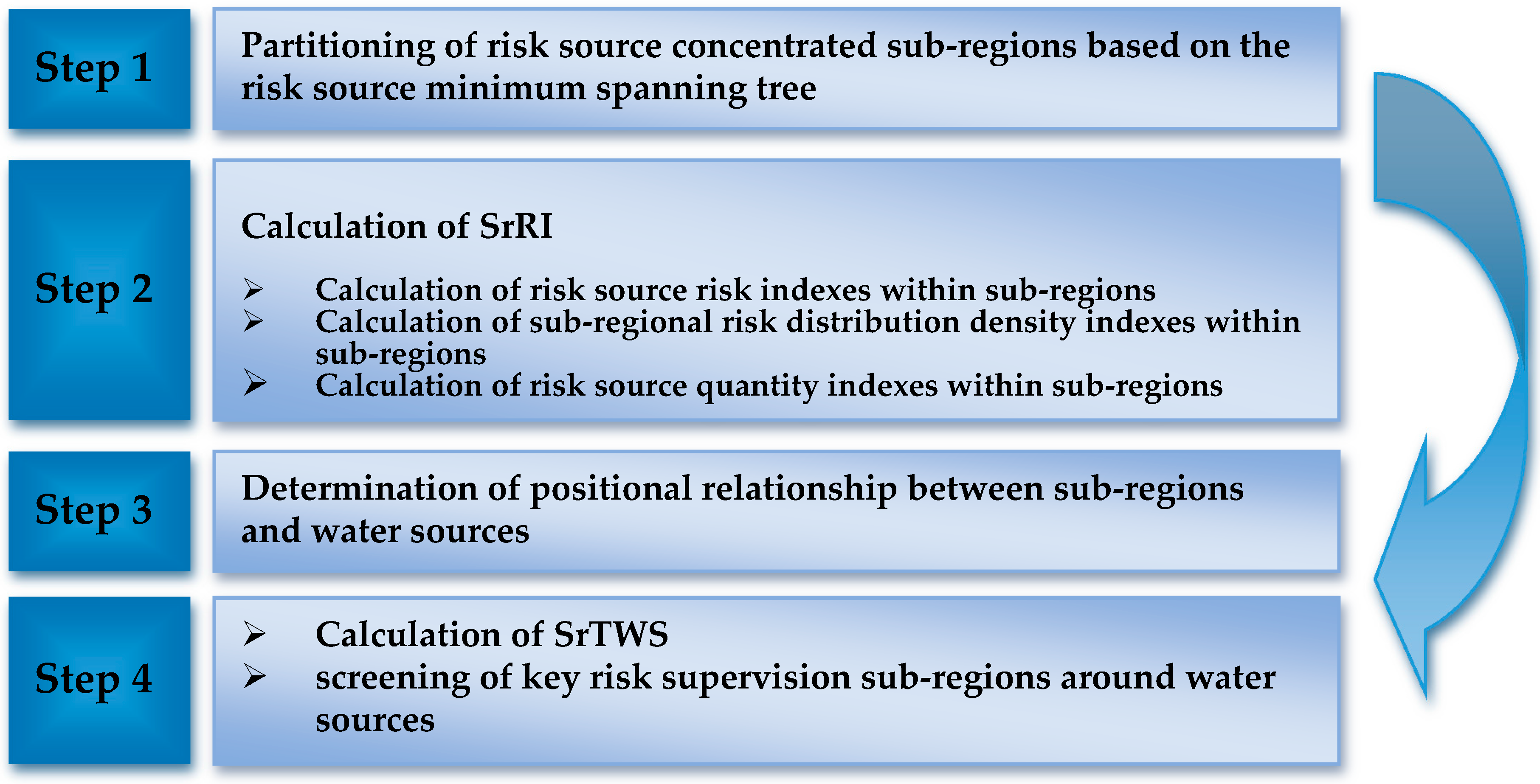
3.1. Minimum Spanning Tree (MST)-Based Method for Partitioning Risk Source Concentrated Sub-Regions

When the risk sources are regarded as the nodes and the lengths of lines linking them are regarded as the weighs, all of the lines linking risk sources constitute a weight map. If we want to connect all the nodes in the weight map with the least number of links, the links selected will have to form a tree [21]. By comparing a certain distance threshold to the distance between two adjacent risk sources on the spanning tree (i.e., weight of the two risk sources), we can determine whether these two risk sources are within the same sub-region. Among all spanning trees, the one with the minimum weighted sum is the minimum spanning tree [21]. Therefore, it is most accurate to determine whether the adjacent risk sources are within the same sub-region based on the distance between adjacent risk sources on the minimum spanning tree.

If a risk source and its adjacent risk sources are within the same sub-region, the distance between it and its adjacent risk sources should be within a certain threshold; and the minimum distances between risk sources within this sub-region and risk sources within other sub-regions should all be greater than this threshold. A typical example is the risk source f₄ as shown in Figure 3a. Its distances from the risk sources f₅ and f₆ are 1.14 km and 1.62 km, respectively (

Table 1. Construction results of risk source minimum spanning tree.

Steps	Node Path	Risk Sources Linked by Paths		Nodal Distance/km	Set of Risk Sources Linked by Minimum Spanning Tree
		Upper End	Lower End
Step 1	L1	f1	f2	1.89	1, 2
Step 2	L2	f2	f3	2.16	1, 2, 3
Step 3	L3	f2	f4	2.74	1, 2, 3, 4
Step 4	L4	f4	f5	1.14	1, 2, 3, 4, 5
Step 5	L5	f4	f6	1.62	1, 2, 3, 4, 5, 6

), while its distance from the risk source f₂ is 2.74 km (Table 1). Assuming a threshold of 2 km, then the risk sources f₄–f₆ should be in the same sub-region, whereas the risk source f₂ is in another sub-region. In addition, there is also the case where the distances between a certain risk source and its adjacent risk sources do not differ much, but some of the distances are slightly greater than the threshold. Various risk sources involved in such case can also be partitioned into one sub-region. A typical example is the risk source f₂ as shown in Figure 3a. Its distances from the risk sources f₁ and f₃ are 1.89 km and 2.16 km, respectively (Table 1). If only compared to the threshold of 2 km, the risk source f₃ should not be partitioned into the same sub-region with sources f₁–f₂. However, since 1.89 km and 2.16 km are not much different, and 2.16 km is only slightly larger than 2 km, we can also consider that the risk sources f₁–f₃ are in the sub-region in this case. Therefore, based on the above analysis, we can determine the sub-region partitioning conditions on the basis of constructing the minimum spanning tree of risk sources by comprehensively considering two aspects: distances between risk source and its adjacent risk sources; and deviation between the distances.

At present, there are already some classic minimum spanning tree algorithms, such as the Kruskal method [22] and the Prim method [23]. In this paper, the Prim algorithm [23] is employed to construct the minimum spanning tree of risk sources. The specific steps are described below. The route between adjacent risk sources on the risk source minimum spanning tree was defined as the node path, whose length was the node distance. With the node distance on the entire risk source minimum spanning tree as the object, if partitioning conditions were satisfied, the corresponding node path would be interrupted. Accordingly, the original single risk source minimum spanning tree would be divided into several minimum spanning trees. Risk sources connected in series by each resulting minimum spanning tree was partitioned into one sub-region.

3.1.1. Construction of Risk Source Minimum Spanning Tree

Prim algorithm [23] was used to construct the risk source minimum spanning tree by assuming there were n number of risk sources in the survey area around water source, and the risk source set was F = {f₁, f₂, … , f_n}. The specific steps were as follows:

(1)

Risk source minimum spanning tree connected the risk sources within the entire survey area in series gradually. The risk source set that had been serially connected by the minimum spanning tree was set as V; the risk source set yet to be serially connected by the minimum spanning tree was set as U; and the node path set on the minimum spanning tree was set as L. Initially, V = { }, U = F, L = { }.

(2)

f_i was added to V starting from any risk source f_i.

(3)

Risk source f_j nearest to all risk sources in V was found from U, and the node path of f_j serially connected by minimum spanning tree was added to L.

(4)

f_j was added to V, U = F − V.

(5)

Steps (3) and (4) were repeated until U = { }.

Specific calculation formula for risk source spacing was as follows:

$$d_{ij}=\sqrt{{(f_{ix}-f_{jx})}^2+{(f_{iy}-f_{jy})}^2}$$

(1)

where f_ix and f_iy are the x and y coordinates of risk source f_i; and f_jx and f_jy are the x and y coordinates of risk source f_j, respectively.

3.1.2. Judgment Criteria for Sub-Region Partition

From the perspective of the entire survey area, whether two risk sources could be partitioned into the same sub-region depended on the contrast of distance between them to the entire survey area size. If the distance between the two was very small relative to the entire survey area, the two risk sources could be partitioned together. Otherwise, the two risk sources should be subordinate to different sub-regions. Thus, when determining the partitioning distance threshold d_min for judging whether two risk sources were within the same sub-region, the size of the entire survey area should be taken into account.

Risk sources posing threat to water sources were generally distributed along the shoreline. Overall, the spatial size of survey area could be represented by the unilateral shoreline length S of the river in the survey area where the water source was located. Ratio of d_min to S was set as 0.1, then:

$$d_{\min }=0.1\cdot S$$

(2)

According to the provision of the Ministry of Environmental Protection’s Guidelines for Protection of Centralized Drinking Water Source Environment [24], the risk source survey area around water sources covers a 20 km range of upstream of secondary water source protection area. In this paper, S was set as 20 km, so d_min was 2 km.

In addition, if the ratio d_i/d_j of node distances d_i and d_j corresponding to two connected node paths L_i and L_j was within a certain range, the ratio range could be set between [0.83, 1.2]. When d_i/d_j ∈ [0.83, 1.2], and one of the node distances was less than or equal to d_min, the three risk sources connected in series by L_i and L_j were partitioned into one sub-region.

Taking into comprehensive consideration the distance between nodes and the deviation between distances of their interconnected nodes, the judgment criteria for sub-region partition were set as follows:

$$\begin{array}{l}{d}_i>d_{\min },\mathrm{and},\frac{d_i}{d_j}>1.2;\mathrm{or}\\ d_i>d_{\min },\mathrm{and},d_j>d_{\min }\end{array}$$

(3)

where d_i is the node distance of node path L_i; L_j is the node path with the largest node distance from L_i, and d_j is its node distance.

3.1.3. Sub-Region Partitioning Procedure

(1)

Prim algorithm [23] was used to construct the risk source minimum spanning tree by assuming there were n number of risk sources in the survey area around water sources. Node path set of the minimum spanning tree was defined as L = {L₁, L₂, …, L_n−1}, while the node distance set corresponding to node paths was defined as D = {d₁, d₂, …, d_n−}.

(2)

Node distance d_i was determined one by one from large to small for whether it satisfied the Equation (3). If satisfied, the node path L_i would be interrupted. Accordingly, the minimum spanning tree where L_i was located was decomposed into two minimum spanning trees.

(3)

Risk sources connected in series by the resulting minimum spanning trees were partitioned into one sub-region.

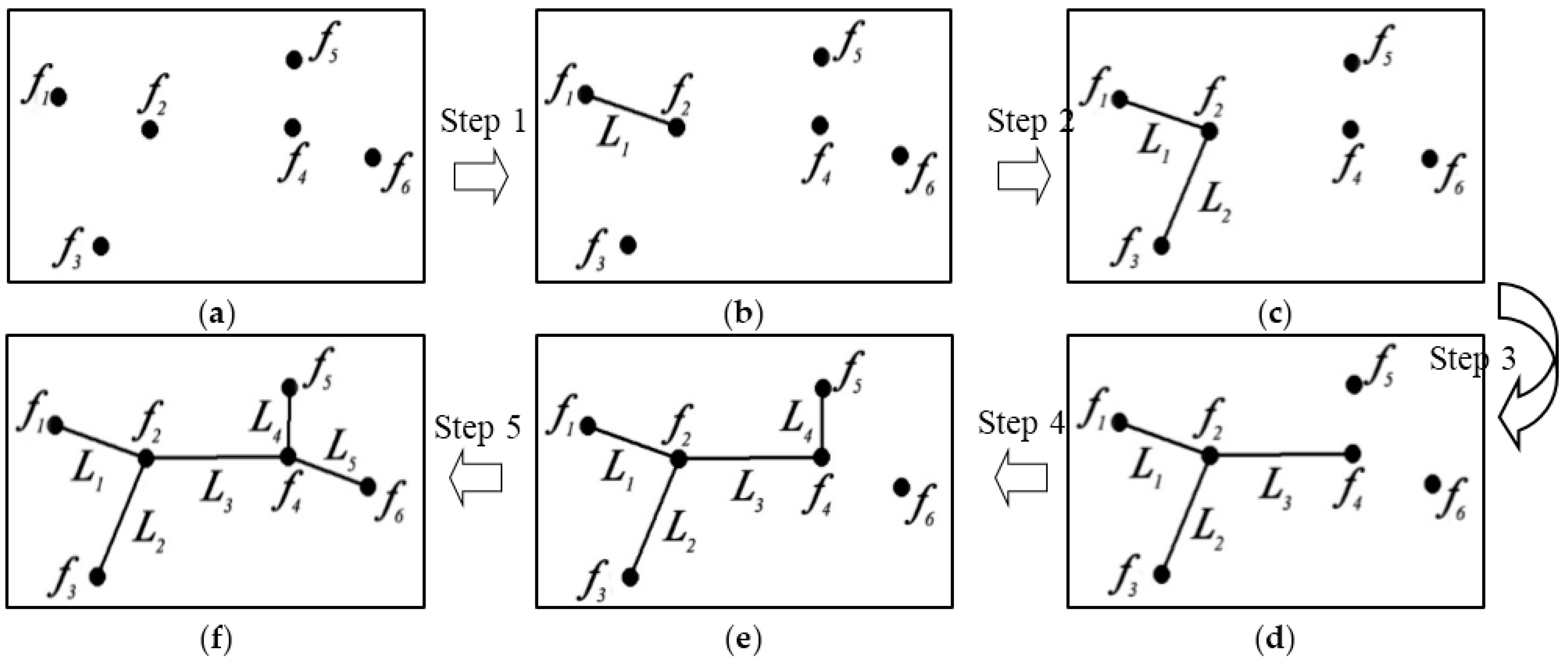
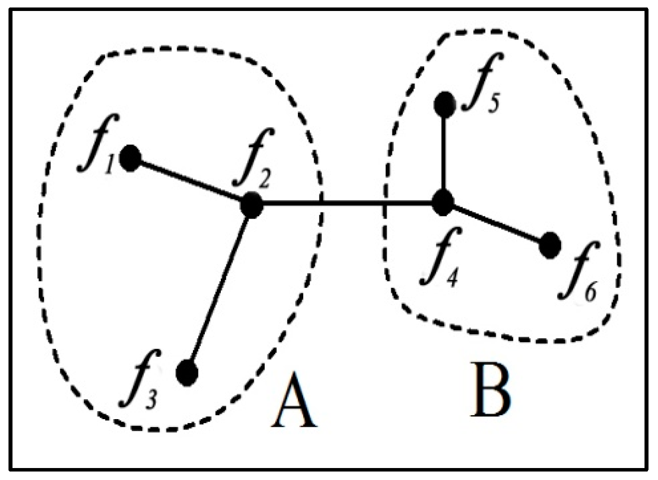
3.1.4. Example of Sub-Region Partitioning

Taking the risk sources f₁–f₆ in Figure 3a as an example, the risk source minimum spanning tree was constructed from the risk source f₁. The construction process and results are shown in Figure 3 and Table 1, whereas the minimum spanning tree of risk source constructed is shown in Figure 4.

By comparing the various path distances in Table 1 to the distance threshold 2 km, it was observed that the paths L₂ and L₃ were both greater than the distance threshold. However, the nodal distance ratio of paths L₂ to L₁ (node path with the largest nodal distance from L₂) was 1.14, while the nodal distance of L1 was 1.89, which was less than the distance threshold. Thus, L₂ did not satisfy Equation (3), and only path L₃ satisfied the interrupt condition. Through interrupting path L₃, two sub-regions could be obtained, of which risk sources f₁–f₃ were partitioned into a sub-region A, and risk sources f₄–f₆ were partitioned into another sub-region B. The specific partitioning results are shown in Figure 4.

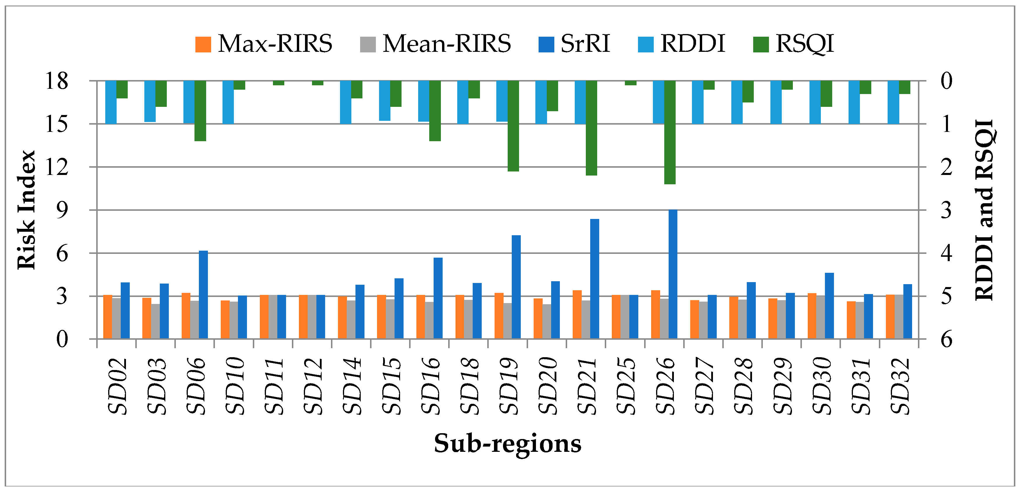
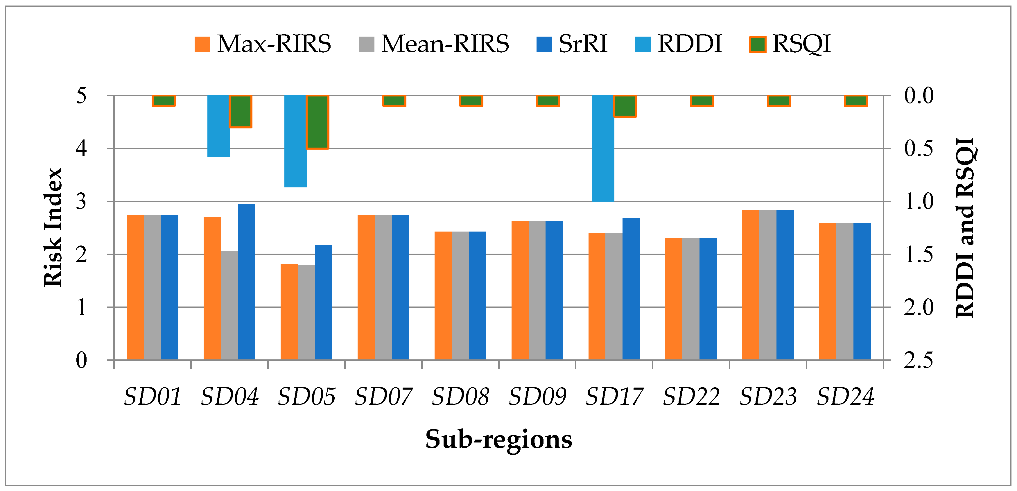
3.2. Method for Determining Sub-Regional Risk Indexes

Determination of SrRI should be based on the RIRS of individual risk sources within the sub-regions. Without considering other influencing factors, the greater the mean value about risk indexes of risk sources (Mean-RIRS) in sub-regions, the greater the value of SrRI theoretically. In addition, considering that risk sources with larger RIRS had far greater risk impact on the sub-regions than those with smaller RIRS, the maximal value about risk indexes of risk sources (Max-RIRS) in sub-regions should also be taken into account in determining SrRI. However, consideration of the effects of RIRS for various risk sources in the sub-regions only was unable to accurately reflect SrRI. If RIRS for individual risk sources in the sub-regions were the same, the larger the number of risk sources in the sub-regions, the greater the sum of RIRS, the higher the risk threats to the surrounding waters, and the greater the SrRI theoretically. Therefore, besides RIRS for various risk sources in the sub-regions, the influences of risk source number on SrRI, and the intensive industrial distribution and close distance between risk sources in the economically developed areas need to be considered. Hence, in case of fire, explosion or other accidents at a risk source, sequential fire or explosion at multiple risk sources may be triggered (such as the Tianjin Port explosion that occurred in August 2015). Compared to the fire or explosion accidents at a single risk source, sequential fire or explosion at multiple risk sources will greatly increase the probability of water pollution accidents. Consequently, when determining SrRI, the concentration degree of risk source distribution in sub-regions should also be considered.

Based on the above analysis, determination of sub-regional risk indexes needs to take into account factors such as Mean-RIRS, Max-RIRS, number of risk sources and degree of risk concentration within a sub-region. The specific calculation formula was as follows:

$$K_t=\underset{1\le i\le m}{\max }(k_{ti})\cdot (1+G_t\cdot D_t\cdot \frac{\overline{k_t}}{k_{\max }})$$

(4)

where K_t is the risk index of the t-th sub-region; and m is the number of risk sources in the t-th sub-region. $\overline{k_t}$ and k_ti are the average risk index of risk sources and the risk index of i-th risk source in the t-th sub-region, respectively. They reflected the risk scale of individual risk sources within a sub-region. k_max is the maximum value that the risk index of individual risk sources could assume. G_t is the risk distribution density index (RDDI) of the t-th sub-region, which reflected the relative degree of risk concentration in the t-th sub-region. D_t is the risk source quantity index (RSQI) of the t-th sub-region, which reflected the risk increment in the t-th sub-region caused by increased number of risk sources.

3.2.1. Method for Determining RIRS

RIRS should be determined by comprehensively considering influential factors such as industry type, production scale, technological level, wastewater complexity and risk supervision and emergency response capability [25]. However, most of the above factors can only be qualitatively described for their scale of risk threats to the surrounding areas except for the production scale (industrial source can be represented by wastewater discharge capacity, and wharf source can be represented by berthing capacity). Hence, it can hardly be quantitatively determined. In contrast, the semi-quantitative comprehensive index method is based on the calculation of a comprehensive evaluation index that summarizes the indexes of multiple risk elements using weight values [15]. This semi-quantitative method has been widely used to assess the risk of chemical and petrochemical areas [18] and mining areas [26]. Therefore, in this paper, RIRS can be assessed employing the comprehensive index method. The specific assessment steps were as follows: (1) Each assessment index of individual risk sources was graded according to relevant risk grading criteria and scored. The risk levels were classified into four categories: very low, low, medium and high, which corresponded to fours scores: 1, 2, 3 and 4, respectively; (2) RIRS were determined by weighted summation based on the weight and score values of indexes. Since the sum of index weights was 1, and the maximum score for each index was 4, the maximum value reachable by RIRS was 4, i.e., k_max = 4. The risk grading criteria and specific weights of indexes are shown in

Table 2. Risk source and sub-regional risk grading criteria.

Risk Level	High	Medium	Low	Very Low
Risk index	≥3	[2, 3)	[1.5, 2)	[1, 1.5)

[25]. Risk levels of risk sources were determined according to the RIRS based on Table 2 [25]. Table 2 could also be used as the sub-regional risk grading criteria.

3.2.2. Method for Determining Sub-Regional RDDI

RDDI of multiple risk sources within sub-region was determined based on the relative degree of risk concentration between adjacent risk sources on the risk source minimum spanning tree.

Relative degree of risk concentration between adjacent risk sources connected by the i-th node path L_ti on the risk source minimum spanning tree in the t-th sub-region could be determined by comparing the node distance d_ti corresponding to L_ti with the risk distance threshold d_max. The specific formula was as follows:

$$w_{ti}=\{\begin{array}{l}1,\mathrm{if}{d}_{ti}\le d_{\max };\\ d_{\max }/d_{ti},\mathrm{if}{d}_{ti}>d_{\max }\end{array}$$

(5)

where w_ti is the index reflecting the relative degree of risk concentration between adjacent risk sources connected by the node path L_ti, and w_ti ∈ (0,1]. When w_ti was equal to 1, it indicated that the two risk sources were completely concentrated; otherwise, it indicated relative concentration. The closer the value of w_ti to 0 was, the lower the degree of concentration between two risk sources would be.

Risk distance threshold d_max was determined based on the length of unilateral river shoreline S reflecting the spatial size of survey area. The specific formula was as follows:

$$d_{\max }=0.05\cdot S$$

(6)

Ministry of Environmental Protection’s Guidelines for Protection of Centralized Drinking Water Source Environment [27] provides that the risk source survey area around water sources covers a 20 km range of upstream of secondary water source protection area. S was considered as 20 km, so d_max was considered as 1 km.

The RDDI of the t-th sub-region was calculated as follows:

$$G_t=\frac{{\displaystyle \sum _{i=1}^{m-1}{w}_{ti}\cdot k_{ti}^u\cdot k_{ti}^d}}{{\displaystyle \sum _{i=1}^{m-1}{k}_{ti}^u\cdot k_{ti}^d}}$$

(7)

where G_t is the RDDI of the t-th sub-region, and G_t∈(0, 1]. The closer the value of G_t to 0, the more dispersed the risks in the t-th sub-region, and vice versa. $k_{ti}^u$ and $k_{ti}^d$ denote the risk indexes of risk sources at the upper and lower ends of node path L_ti, respectively. Meanings of m and w_ti are the same as above.

3.2.3. Method for Determining Sub-Regional RSQI

If the impact of risk source risk indexes was not considered, the more the number of risk sources within sub-region, the greater the water environmental risk in the sub-region. RSQI was determined by assuming that the increment of risk source quantity in the t-th sub-region was linearly related to the increment of sub-regional risk. Specific formula was shown below:

$$D_t=m/10$$

(8)

where D_t and m have the same meanings as above.

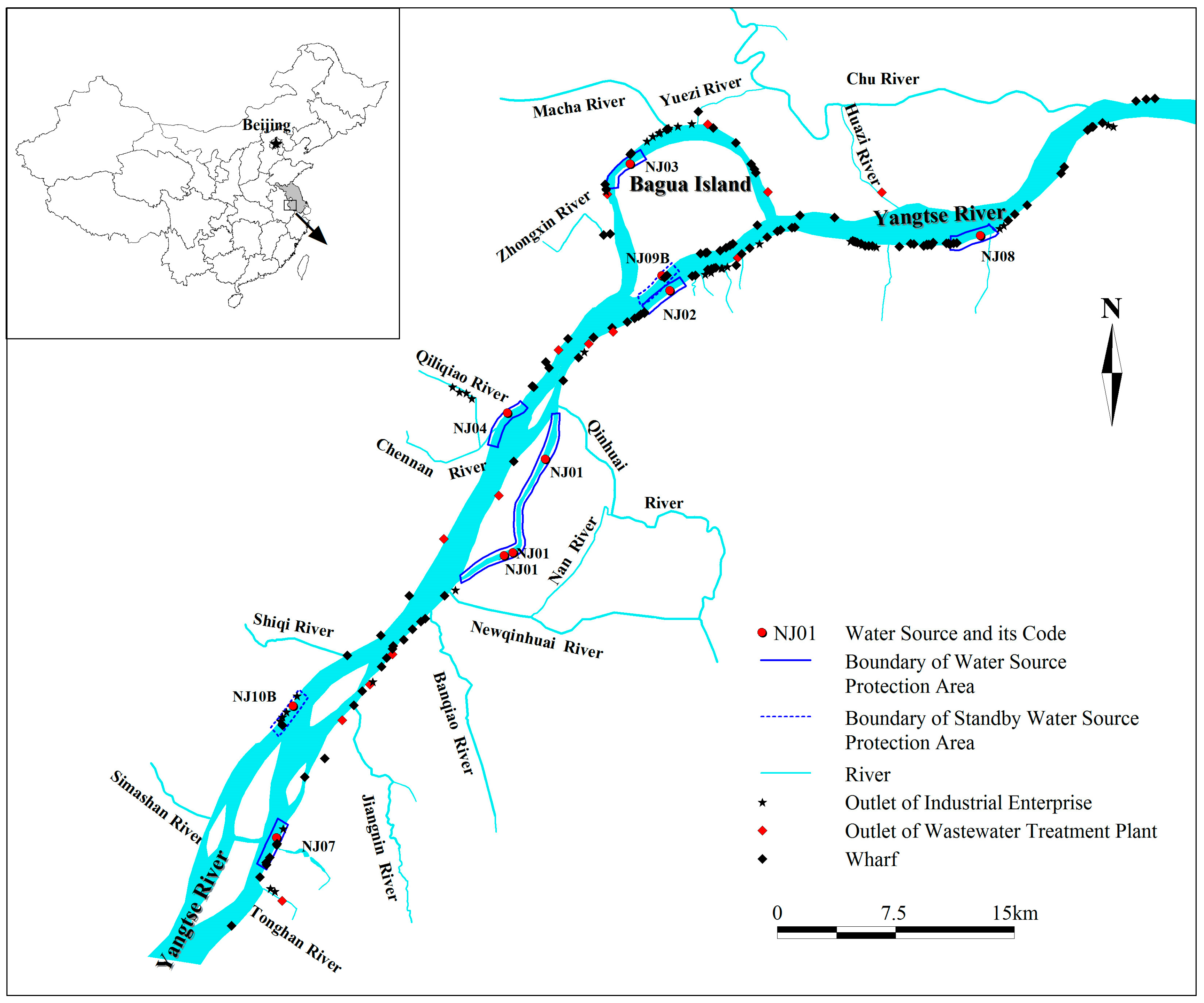
3.3. Method for Determining Water Source Perimeter Key Risk Supervision Sub-Regions

Determination basis of key risk supervision sub-regions around water sources was the sub-region’s scale of risk threats to the water sources. In contrast, the aforementioned sub-regional risk index characterized the sub-region’s scale of risk threats to its surrounding water environment sensitive receptors. The larger the SrRI, the severer the substandard condition of water for sensitive waters after pollution accidents, and the greater the risk threats to these sensitive waters. In this case, the receptor should be close to the sub-region. If the distance between the two increased, the sub-region’s risk threats to the sensitive receptor should be reduced. Similarly, whether the sub-region and sensitive receptor were on the same shoreline; and whether the sub-region was located upstream of sensitive receptor would also impact the sub-region’s scale of threats to the receptor.

Based on the above analysis, SrTWS was determined in this paper via the SrRI and the positional relationship between sub-region and water source. The positional relationship between sub-region and water source includes: distance between the sub-region and the water source in the direction of water body’s forward flow, i.e., the x directional distance; whether the sub-region and the water source were on the same shoreline, if not, distance between the two in the vertical direction of water body’s forward flow, i.e., the y directional distance; and in the case of reciprocating flow of water body, the upstream–downstream positional relationship between the sub-region and the water source.

Sub-regional risk supervision level was determined according to SrTWS, thereby identifying the key risk supervision sub-regions around water sources. Risk supervision grading criteria were established based on the risk grading criteria for risk sources [25]. The details are shown in

Table 3. Sub-regional risk supervision grading criteria.

Sub-Regional Risk Supervision Level	Key Supervision	Secondary Key Supervision	Non-Key Supervision
SrTWS	≥3	[1.5, 3)	<1.5

.

Specific calculation formula for SrTWS was as follows:

$$W{G}_t=G_t\cdot X_t\cdot Y_t\cdot P_t$$

(9)

where WG_t is the t-th sub-region’s SrTWS; and X_t and Y_t, are the adjustment coefficients determined by considering the magnitudes of distances between the t-th sub-region and the water source in the x and y directions, respectively. When the sub-region and the water source were located on the same shoreline, Y_t was 1. P_t was the adjustment coefficient considering the upstream–downstream positional relationship between the t-th sub-region and the water source. G_t had the same meaning as above.

According to the provision of the Ministry of Environmental Protection’s Guidelines for Protection of Centralized Drinking Water Source Environment [24], the risk source survey area around water sources covers a 20 km range of upstream of secondary water source protection area. In this paper, SrTWS was considered equal to the sub-regional risk index when the x directional distance between sub-region and secondary water source protection area was within 10 km irrespective of other factors. When the x directional distance between sub-region and secondary water source protection area was greater than 10 km, SrTWS decreased linearly with the increasing distance. X_t was determined according to this principle, and its calculation formulas were:

$$X_t=\{\begin{array}{l}1,\mathrm{if}\left|S_{tx}\right|-LW<10;\\ \frac{10}{\left|S_{tx}\right|-LW},\mathrm{if}\left|S_{tx}\right|-LW>10\end{array}$$

(10)

$$S_{tx}=\frac{{\displaystyle \sum _{i=1}^m(s_{tix}\cdot k_{ti})}}{{\displaystyle \sum _{i=1}^m(k_{ti})}}$$

(11)

where S_tx is the integrated distance (km) from multiple risk sources within the t-th sub-region to water intake in the x direction. If the t-th sub-region was located upstream of the water source, S_tx > 0; otherwise, S_tx < 0. LW was the distance (km) from source water intake to the upstream and downstream secondary protection area boundary. When the sub-region was located downstream of the water source, the value of LW was the distance from water intake to downstream secondary protection area boundary. m was the number of risk sources within the t-th sub-region. s_tix, k_ti were the x directional distance (km) from i-th risk source within t-th sub-region to water intake and the risk index of i-th risk source, respectively. When the risk source was located upstream of the water source, the value of s_tix was positive; otherwise, the value was negative. X_t had the same meaning as above.

As the lateral flow of the river was small, the sub-regions located on the other shore of water sources had less threat on the water sources. Similarly, reflected in the setting of water source protection areas, the width of protection areas should be significantly less than their length. By referring to the method of determining X_t coefficient, Y_t in the case where sub-region and water source were not on the same shoreline was determined with protection area width as the standard. The specific calculation formulas were as follows:

$$Y_t=\{\begin{array}{l}1,\mathrm{if}{S}_{ty}\le W{I}_p;\\ W{I}_p/S_{ty},\mathrm{if}{S}_{ty}>W{I}_p\end{array}$$

(12)

$$S_{ty}=\frac{{\displaystyle \sum _{i=1}^m(s_{tiy}\cdot k_{ti})}}{{\displaystyle \sum _{i=1}^m(k_{ti})}}$$

(13)

where S_ty and WI_p were the y directional integrated distance (km) from the t-th sub-region to the shoreline of water source location and the width (km) of secondary water source protection area at the source water intake; respectively. s_tiy was the y directional distance (km) from i-th risk source within t-th sub-region to water intake. Y_t and k_ti had the same meanings as above.

For reciprocating flow, the sub-regions located downstream of water sources only posed risk threats on the water sources through reverse flow, whose risk threats were smaller compared to the sub-regions upstream of water sources. The influence of the upstream–downstream positional relationship between sub-regions and water sources on the SrTWS could be reflected by the forward and reverse flow durations of water sources. The specific formula was as follows:

$$P_t=\{\begin{array}{l}1,\mathrm{if}{S}_{tx}>0;\\ T_O/T_F,\mathrm{if}{S}_{tx}<0.\end{array}$$

(14)

where T_F and T_O are the forward and reverse flow durations of water source, respectively; and P_t has the same meaning as above.

4. Results and Discussion

4.1. Sub-Region Partitioning Results

Risk source minimum spanning tree was constructed using Prim algorithm [23] with the risk sources distributed along the Yangtze’s Nanjing section as the nodes. Meanwhile, risk source-distributed sub-regions were partitioned. Figure 5 presents the risk source minimum spanning tree and the sub-region partition results. As shown in the figure, risk sources distributed along the Yangtze’s Nanjing section can be partitioned into 32 sub-regions from SD01 to SD32. The major risk source-concentrated sub-regions were SD06, SD16, SD19, SD21 and SD26, which contained 14, 14, 21, 22 and 24 risk sources, respectively. In terms of distribution location, except for the sub-region SD06 which was located in the Jiangning Binjiang Industrial Park upstream of Nanjing’s main urban district, the other four major sub-regions were located in the Xiaguan Port District, Luhe Chemical Park’s riverside portion, Xinshengwei Foreign Trade Harbor District and Longtan Port District downstream of Nanjing’s main urban district. Among them, sub-regions SD16 and SD26 were closely neighboring the downstream water source NJ02 and NJ08 protection areas. The remaining sub-regions were smaller than the above-mentioned five major sub-regions, with each containing 1–6 risk sources. Among them, sub-regions SD03, SD05, SD27 and SD32 were distributed within the protection areas of water sources NJ07, NJ10B, NJ08 and NJ09B, respectively.

4.2. Calculation Results of SrRI

A total of 170 risk sources were surveyed. The level and score of assessment indexes for each risk source were determined by referring to Appendix A

Table A2. Risk assessment index system for risk sources [25].

Type of Risk Source	Assessment Index	Risk Grading Criteria for Indexes				Index Weight
		High	Medium	Low	Very Low
Industrial enterprises and sewage treatment plants	Industry type	Petrochemical, coking and nuclear fuel processing, chemical, pharmaceutical enterprises and sewage treatment plants	Textiles, paper, metal smelting and rolling processing, metal surface treatment and heat treatment processing, leather manufacturing, rubber and plastic products, chemical fiber enterprises	Equipment manufacturing, communication and transportation, storage and postal, construction, mining enterprises	Others	0.207
	Complexity of sewage quality	Complex	Medium	Simple	No discharge	0.159
	Wastewater discharge (m3∙day−1)	>2000	(1000, 2000]	(200, 1000]	≤200	0.182
	Technology level of production equipment	Domestically backward	Domestically average	Domestically advanced	Internationally advanced	0.128
	Management system	Incomplete	Comprehensive but unreasonable	Comprehensive and reasonable	Comprehensive, reasonable and well implemented	0.128
	Emergency prevention system	No emergency plan or environmental risk assessment	Either emergency plan or environmental risk assessment	Both emergency plan and environmental risk assessment, but no regular exercise	Both emergency plan and environmental risk assessment, with regular exercise	0.098
	Section monitoring system	No automatic water pollution detector	Installed with automatic water pollution detector, but without detection ability	Installed with automatic water pollution detector, and capable of conducting some tests	Installed with automatic water pollution detector, and capable of conducting comprehensive tests	0.098
Wharf	Type of wharf	Petrochemical, chemical wharfs	Bulk and general cargo, power plant, coal ash wharfs	Containers, outfitting, materials wharfs	Others	0.236
	Berthing capacity (t)	>40,000	(20,000, 40,000]	(5000, 40,000]	≤4000	0.204
	Technology level of production equipment	Domestically backward	Domestically average	Domestically advanced	Internationally advanced	0.161
	Management system	Incomplete	Comprehensive but unreasonable	Comprehensive and reasonable	Comprehensive, reasonable and well implemented	0.161
	Emergency prevention system	No emergency plan or environmental risk assessment	Either emergency plan or environmental risk assessment	Both emergency plan and environmental risk assessment, but no regular exercise	Both emergency plan and environmental risk assessment, with regular exercise	0.128
	Section monitoring system	No automatic water pollution detector	Installed with automatic water pollution detector, but without detection ability	Installed with automatic water pollution detector, and capable of conducting some tests	Installed with automatic water pollution detector, and capable of conducting comprehensive tests	0.11

. RIRS of various risk sources were determined by weighted summation based on the risk scores and weights of indexes (see Appendix A Table A2). Meanwhile, risk levels of risk sources were determined according to Table 2. Risk assessment results revealed that 29 of 170 risk sources were high risk sources, which were mainly wastewater treatment plants’ outlets (15) and wharf risk sources (11). The 11 high-risk wharf loading and unloading articles were oils, bulk toxic liquids, etc. None of these wharfs were equipped with automatic water quality detector or pollution control facility, whose sensitivity and emergency response to sudden pollution accidents were poor. Among them, wharfs njm47, njm83, njm85, njm89 and njm90 all had a berthing capacity above 40,000 t. Therefore, RIRS of these five wharfs were the highest, which were all 3.389 (risk scores for six indexes: wharf type, wharf berthing capacity, technological level of production equipment, management system, emergency prevention system and section monitoring system were 4, 4, 3, 2, 3, and 4, respectively). Jingling Sinopec’s first chemical plant (code 271) scored the second highest (3.359) for RIRS due to high industry risk and high complexity of wastewater discharged (for the seven indexes of the industry type, complexity of sewage quality, wastewater discharge, technological level of production equipment, management system, emergency prevention system and section monitoring system, the risk scores were 4, 3, 4, 3, 2, 3, and 4, respectively). As its annual wastewater discharge was nearly 830,000 t, its RIRS was higher than the other two high risk enterprises (both of which were petroleum processing enterprises with RIRS of both 3.197. For the seven indexes of the industry type, sewage quality complexity, wastewater discharge, production equipment level, management system, emergency prevention system and section monitoring system, the risk scores were 4, 3, 1, 4, 4, 3, 4, respectively). All 15 wastewater treatment plants distributed along the Yangtze’s Nanjing section were high risk sources. Although annual wastewater discharge of each plant was at least 1,800,000 t, their discharge complexity was lower than the above-mentioned three high risk enterprises since they primarily deal with domestic wastewater. Moreover, they all had certain water quality monitoring capability. Thus, overall, the RIRS of wastewater treatment plants were slightly lower than the high-risk enterprises. Specific locations of high risk sources are shown in Figure 5. The specific RIRS results for high risk sources are listed in

Table 4. RIRS calculation results for high risk sources.

Sub-Region	Risk Source			Sub-Region	Risk Source
	Code	Location	RIRS		Code	Location	RIRS
SD02	W026	118.541°E, 31.798°N	3.065	SD25	W035	118.942°E, 32.199°N	3.065
SD06	W030	118.580°E, 31.900°N	3.065	SD26	njm83	118.928°E, 32.170°N	3.389
	W016	118.597°E, 31.921°N	3.224		njm84	118.933°E, 32.165°N	3.099
	W015	118.614°E, 31.938°N	3.065		njm85	118.934°E, 32.165°N	3.389
SD11	W012	118.649°E, 32.000°N	3.065		njm89	118.928°E, 32.173°N	3.389
SD12	W002	118.684°E, 32.028°N	3.065		njm90	118.961°E, 32.170°N	3.389
SD15	W011	118.725°E, 32.109°N	3.065		njm101	118.973°E, 32.169°N	3.099
SD16	W003	118.746°E, 32.113°N	3.065		njm127	118.987°E, 32.170°N	3.099
	W033	118.761°E, 32.120°N	3.065	SD30	377	119.093°E, 32.237°N	3.197
SD18	W010	118.758°E, 32.198°N	3.065		378	119.097°E, 32.236°N	3.197
SD19	W048	118.825°E, 32.238°N	3.224	SD32	njm123	118.796°E, 32.151°N	3.099
	W044	118.865°E, 32.220°N	3.065		njm124	118.797°E, 32.151°N	3.099
SD21	njm47	118.883°E, 32.179°N	3.389		njm125	118.798°E, 32.152°N	3.099
	271	118.834°E, 32.156°N	3.359
	W013	118.845°E, 32.162°N	3.065
	W014	118.846°E, 32.162°N	3.065

.

SrRI were calculated based on the RIRS and locations of various risk sources; meanwhile, sub-regional risk levels (SrRL) were assessed. As shown in

Table 5. Sub-regional risk index calculation results.

Sub-Region	RDDI	RIRS		RSQI	SrRI	SrRL
		Maximum	Mean
SD01	0	2.745	2.745	0.1	2.745	Medium
SD02	1	3.065	2.850	0.4	3.939	High
SD03	0.954	2.863	2.441	0.6	3.862	High
SD04	0.581	2.702	2.060	0.3	2.944	Medium
SD05	0.865	1.817	1.801	0.5	2.171	Medium
SD06	0.976	3.224	2.663	1.4	6.158	High
SD07	0	2.745	2.745	0.1	2.745	Medium
SD08	0	2.429	2.429	0.1	2.429	Medium
SD09	0	2.633	2.633	0.1	2.633	Medium
SD10	1	2.683	2.612	0.2	3.033	High
SD11	0	3.065	3.065	0.1	3.065	High
SD12	0	3.065	3.065	0.1	3.065	High
SD13	0	1.739	1.739	0.1	1.739	Low
SD14	1	2.981	2.690	0.4	3.783	High
SD15	0.923	3.065	2.760	0.6	4.236	High
SD16	0.942	3.065	2.579	1.4	5.670	High
SD17	1	2.397	2.397	0.2	2.684	Medium
SD18	1	3.065	2.733	0.4	3.903	High
SD19	0.942	3.224	2.511	2.1	7.227	High
SD20	1	2.831	2.428	0.7	4.034	High
SD21	1	3.389	2.679	2.2	8.382	High
SD22	0	2.305	2.305	0.1	2.305	Medium
SD23	0	2.831	2.831	0.1	2.831	Medium
SD24	0	2.591	2.591	0.1	2.591	Medium
SD25	0	3.065	3.065	0.1	3.065	High
SD26	0.985	3.389	2.815	2.4	9.025	High
SD27	1	2.713	2.611	0.2	3.067	High
SD28	1	2.949	2.755	0.5	3.965	High
SD29	1	2.831	2.713	0.2	3.215	High
SD30	1	3.197	2.965	0.6	4.619	High
SD31	1	2.633	2.578	0.3	3.142	High
SD32	1	3.099	3.099	0.3	3.819	High

, among the 32 sub-regions, those with high, medium and low risk levels were 21, 10 and 1, respectively. The only low-risk sub-region was SD13, within which there was only one low-risk source, a public dock.

Statistical analysis chart (Figure 6) of SrRI in the high risk sub-regions was plotted. As can be seen, compared to other high risk sub-regions, the sub-regions SD06, SD16, SD19, SD21 and SD26 exhibited significantly larger SrRI owing to their advantages in quantity and RIRS (risk sources with the highest and the second highest RIRS were located in sub-regions SD26 and SD21, respectively). Although the sub-regions SD11, SD12 and SD25 each had only one risk source compared to other high risk sub-regions, they were also listed as high risk sub-regions as the risk sources were large-scale wastewater treatment plants. Nevertheless, their SrRI were slightly smaller than other high risk sub-regions. Although all the risk sources in the sub-regions SD10, SD20, SD27, SD29 and SD31 were medium risks (Max-RIRS of less than 3), SrRI of these sub-regions were greater than 3 due to a certain number of concentrated risk sources within each sub-region, which made them high risk sub-regions.

Statistical analysis chart (Figure 7) of SrRI in the medium risk sub-regions was drawn. Most of the medium risk sub-regions contained only 1 medium risk source. In the medium risk sub-regions SD04, SD05 and SD17, there were slightly more risk sources (3, 5 and 2, respectively). Although the risk sources in the sub-region SD17 were concentrated, the RIRS was small and there were only two risk sources, so the SrRI was also not too large. Since the risk sources were relatively dispersed in the two sub-regions SD04 and SD05, the SrRIof these two sub-regions were not large. Compared to other medium risk sub-regions, sub-region SD05 exhibited the smallest SrRI despite multiple risk sources because the risk sources within it were small-scale shipyards and public docks.

4.3. Determination of Key Risk Supervision Sub-Regions

The x and y directional distances from sub-regions to source water intakes were determined based on the risk indexes and locations of risk sources. Appendix A

Table A3. Integrated distances from sub-regions to source water intakes. Unit: km.

Sub-Region	NJ07		NJ10B		NJ01		NJ02		NJ03		NJ04		NJ08		NJ09B
	x	y	x	y	x	y	x	y	x	y	x	y	x	y	x	y
SD01	6.39	0	13.08	1.33	29.83	0	50.08	0	57.25	0.88	37.63	1.33	71.01	0	51.34	1.33
SD02	3.32	0	10.82	1.46	26.97	0	47.17	0	54.24	1.01	35.1	1.46	68.19	0	48.83	1.46
SD03	Within the protection area		7.95	1.04	23.02	0	44.45	0	51.33	0.59	32.19	1.04	65.01	0	46.06	1.04
SD04	−5.05	0	0	3.33	18.5	0	38.59	0	45.73	2.88	25.62	3.33	59.54	0	40.68	3.33
SD05	−7.26	2.85	Within the protection area		16.75	2.85	36.77	2.85	43.87	2.85	23.9	0	57.65	2.85	37.94	1.8
SD06	−12.52	0	−5.56	1.47	10.96	0	30.72	0	38.79	1.02	16.65	1.47	50.61	0	30.68	1.47
SD07	−11.89	2.13	−4.67	0	11.66	2.13	31.75	2.13	37.05	2.13	18.52	0	52.57	2.13	32.52	1.08
SD08	−14.31	1.2	−7.16	0	9.3	1.2	29.44	1.2	36.45	1.2	16.03	0	50.22	1.2	30.05	0.15
SD09	−17.33	1.46	−10.29	0	6.25	1.46	26.25	1.46	33.45	1.46	12.97	0	47.18	1.46	26.99	0.41
SD10	−19.7	0	−12.1	1.87	4.25	0	24.39	0	31.55	1.42	11.14	1.87	45.38	0	25.17	1.87
SD11	−22.22	1.74	−14.57	0	-		21.15	1.74	28.45	1.74	8.67	0	42.41	1.74	22.64	0.59
SD12	−26.17	0	−18.67	1.52	-		17.49	0	24.54	1.07	4.65	1.52	38.44	0	18.53	1.52
SD13	−28.46	0	−20.68	1.63	-		15.15	0	22.23	1.18	2.62	1.63	36.05	0	16.39	1.63
SD14	−29.86	5.62	−26.83	0	-		14.53	5.62	20.92	5.62	6.95	0	35.5	5.62	20.25	1.04
SD15	−35.38	1.1	−27.56	0	−5.94	1.1	8.6	1.1	15.48	1.1	−3.76	0	29.39	1.1	9.13	0.05
SD16	−38.78	0	−31.17	1.43	−8.22	0	5.27	0	13.2	0.98	−7.47	1.43	25.95	0	5.82	1.43
SD17	−46.35	0.93	−38.58	0	−16.64	0.93	-		4.72	0.93	−14.65	0	30.67	0.93	-
SD18	−49.15	0.69	−40.88	0	−19.43	0.69	-		0	0.69	−17.1	0	27.85	0.69	-
SD19	−55.66	1.05	−48.37	0	−25.91	1.05	-		−4.51	1.05	−24.27	0	21.3	1.05	-
SD20	−47.43	1.03	−40.81	0	−17.78	1.03	−3.7	1.09	-		−17.3	0	17.41	1.03	−3.93	0
SD21	−48.57	0	−42.27	0.96	−18.95	0	−4.76	0	-		−17.91	0.96	16.16	0	−4.98	0.96
SD22	−50.47	0.96	−44.18	0	−21.04	0.96	−6.94	0.98	-		−20.38	0	13.93	0.96	−7.08	0
SD23	−52.73	1.08	−47	0	−23.21	1.08	−9.24	1.04	−14.06	1.08	−23.22	0	11.76	1.08	−9.81	0.03
SD24	−54.93	1.21	−49.27	0	−25.36	1.21	−11.19	1.3	−16.12	1.21	−25.44	0	9.7	1.21	−12.13	0.16
SD25	−59.35	3.3	−55.11	0	−28.72	3.3	−14.82	0	−20.46	3.3	−31.29	0	5.32	3.3	−17.93	2.25
SD26	−59.73	0	−53.99	2.5	−29.56	0	−15.73	3.54	−19.76	2.05	−30.02	2.5	5.96	0	−15.91	2.5
SD27	−62.67	0	−57.1	1.75	−33.22	0	−19.19	0	−23.94	1.3	−33.27	1.75	Within the protection area		−19.85	1.75
SD28	−66.5	0	−60.17	1.18	−36.89	0	−22.71	0	−27.69	0.73	−36.4	1.18	−2.12	0	−23.62	1.18
SD29	−70.98	0	−63.98	1.92	−41.49	0	−27.46	0	−32.34	1.47	−39.98	1.92	−6.77	0	−26.98	1.92
SD30	−74.52	0	−68.19	1.1	−45.29	0	−31.18	0	−36.31	0.65	−44.83	1.1	−10.41	0	−31.11	1.1
SD31	−77.78	1.28	−72.1	0	−48.3	1.28	−34.12	0.91	−39.35	1.28	−48.3	0	−13.55	1.28	−34.75	0.23
SD32	−43.89	0.95	−37.34	0	−14.63	0.95	0	0.96	-	0	-13.6	0	20.72	0.95	Within the protection area

lists the specific results. In Appendix A Table A3, the x directional distance from sub-region to water intake would be positive if the sub-region was located upstream of the water source; 0 if the sub-region was located within the water source protection area; and negative if located downstream of the water source. The y directional distance from sub-region to water intake would be 0 if the sub-region and the water source were on the same shoreline; and positive if were on the opposite shorelines. Some sub-regions such as SD14 were located in the Yangtze tributaries, so their x directional distances to water intakes were regarded as the sum of distance from sub-region to tributary estuary and distance from the estuary to water intake. Meanwhile, the y directional distance to water intake was considered as the y directional distance from tributary estuary to water intake. In addition, part of the sub-regions did not pose threats to some water sources as a result of island barrier. In such case, the distance from sub-region to water intake was not considered, such as the distances from the sub-regions SD11-SD14 to the water source NJ01 in Appendix A Table A3. According to the Jiangsu Provincial Program for Partitioning County Level or Above Centralized Drinking Water Source Protection Areas [27], the distances from the source water intake to the secondary protection area upstream and downstream boundaries were 2 km and 1 km, respectively, for eight water sources along the Yangtze’s Nanjing section expect for the Jiajiang water source (NJ01), whose corresponding distances were 3.2 km and 3.0 km, respectively. Width of all waters in the secondary protection areas was 0.5 km.

SrTWS were calculated based on the SrRI and the distances from water intakes to secondary protection area boundaries in Table 5 and Appendix A Table A3, respectively. During calculation, the forward and reverse flow durations of water sources were considered according to the durations of ebb and flood in the Yangtze’s Nanjing section, respectively. The calculation results are shown in Appendix A

Table A4. Calculation results of SrTWS.

Sub-Region	SrRI	SrTWS								SD-TSrTWS
		NJ07	NJ10B	NJ01	NJ02	NJ03	NJ04	NJ08	NJ09B
SD01	2.745	2.745	0.931	1.031	0.571	0.282	0.290	0.398	0.209	6.457
SD02	3.939	3.939	1.349	1.657	0.872	0.373	0.407	0.595	0.288	9.480
SD03	3.862	4.000	1.857	1.949	0.910	0.664	0.615	0.613	0.421	11.029
SD04	2.944	0.981	0.442	1.925	0.805	0.117	0.187	0.512	0.114	5.083
SD05	2.171	0.127	4.000	0.281	0.110	0.091	0.991	0.068	0.168	5.836
SD06	6.158	1.782	0.698	6.158	2.144	0.821	1.430	1.267	0.730	15.030
SD07	2.745	0.197	0.915	0.644	0.217	0.184	1.662	0.127	0.416	4.362
SD08	2.429	0.253	0.810	1.012	0.369	0.294	1.731	0.210	0.866	5.545
SD09	2.633	0.184	0.878	0.902	0.372	0.287	2.400	0.200	1.054	6.275
SD10	3.033	0.541	0.244	3.033	1.355	0.361	0.811	0.699	0.350	7.394
SD11	3.065	0.138	0.753	0	0.460	0.333	3.065	0.218	1.258	6.225
SD12	3.065	0.406	0.190	0	1.979	0.635	1.008	0.841	0.610	5.669
SD13	1.739	0.211	0.090	0	1.322	0.364	0.533	0.511	0.371	3.403
SD14	3.783	0.039	0.488	0	0.269	0.178	3.783	0.100	0.997	5.853
SD15	4.236	0.187	0.532	0.642	1.925	1.428	1.412	0.703	4.236	11.065
SD16	5.670	0.500	0.219	1.890	5.670	2.583	0.661	2.367	1.983	15.873
SD17	2.684	0.106	0.238	0.353	0	1.443	0.655	0.503	0	3.299
SD18	3.903	0.196	0.326	0.574	0	2.828	0.808	1.094	0	5.825
SD19	7.227	0.210	0.508	0.501	0	1.147	1.035	1.783	0	5.184
SD20	4.034	0.141	0.338	0.442	0.617	0	0.825	1.271	1.345	4.977
SD21	8.382	0.587	0.353	1.751	2.794	0	0.860	5.919	1.455	13.720
SD22	2.305	0.081	0.178	0.222	0.392	0	0.396	1.006	0.768	3.044
SD23	2.831	0.084	0.205	0.216	0.454	0.334	0.425	1.311	0.944	3.973
SD24	2.591	0.066	0.179	0.160	0.326	0.236	0.353	1.071	0.776	3.167
SD25	3.065	0.027	0.189	0.060	0.739	0.080	0.337	0.464	0.134	2.030
SD26	9.025	0.512	0.114	1.133	0.288	0.391	0.207	9.025	0.404	12.074
SD27	3.067	0.166	0.052	0.338	0.562	0.171	0.091	4.000	0.155	5.535
SD28	3.965	0.202	0.095	0.390	0.609	0.339	0.158	1.321	0.248	3.361
SD29	3.215	0.153	0.044	0.278	0.405	0.116	0.072	1.072	0.107	2.248
SD30	4.619	0.209	0.104	0.364	0.510	0.335	0.160	1.540	0.232	3.455
SD31	3.142	0.053	0.147	0.090	0.174	0.107	0.221	0.326	0.310	1.429
SD32	3.819	0.156	0.350	0.576	1.989	0	1.010	1.074	4.000	9.156
WS-TSrTWS	-	19.179	17.815	28.571	29.207	16.523	28.601	42.210	24.949	-

. Appendix A Table A4 also lists the total risk threats from single sub-region to all water sources (hereinafter referred to as the SD-TSrTWS), the total risk threats from all sub-regions to single water source (hereinafter referred to as the WS-TSrTWS), and SrRI. Since SD03 was located within the protection area of water source NJ07, it was a key supervision sub-region for NJ07 regardless of its SrRI. In Appendix A Table A4, the scale of SrTWS on NJ07 from SD03 was 4. Others, such as the scale of SrTWS on NJ10B from SD05 were also taken as 4. In addition, for water sources not affected by some sub-regions due to the barrier of islands in the river, their SrTWS was taken as 0.

Based on Appendix A Table A4, the key and secondary key supervision sub-regions corresponding to each water source were determined according to the sub-region supervision grading criteria established in Table 3. The results are shown in

Table 6. Key and secondary key supervision sub-regions corresponding to various water sources.

Water Source	Key Supervision Sub-Regions	Secondary Key Supervision Sub-Regions
NJ07	SD03, SD02	SD01, SD06
NJ10B	SD05	SD03
NJ01	SD06, SD10	SD03, SD04, SD16, SD21, SD02
NJ02	SD16	SD21, SD06, SD32, SD12, SD15
NJ03	SD16	SD18
NJ04	SD14, SD11	SD07, SD08, SD09
NJ08	SD26, SD21, SD27	SD16, SD19, SD30
NJ09B	SD15, SD32	SD16

.

Variations of SD-TSrTWS and SrRI for various sub-regions (Figure 8) were plotted in the upstream to downstream order of sub-regions. In the Figure 8, the upstream sub-regions were located to the left of the downstream sub-regions. As shown in Appendix A Table A4 and Figure 8, SD16’s SD-TSrTWS was the maximum, 15.873. Although the SrRI of sub-regions SD26, SD21, SD19 and SD06 were all larger than the sub-region SD16, SD26, SD21 and SD19 were located downstream of the majority of water sources. Besides, SD21 and SD19 were located on the north and south watercourse of the Yangtze’s Bagua Island, respectively, and did not produce risk threat to the water sources that were not on the same watercourse. As for sub-region SD06, although it was located upstream of most water sources, it was distant from most water sources compared to the sub-region SD16. Thus, among five sub-regions with SrRI greater than 5, SD16’s SrTWS to the Nanjing riverside water sources was the greatest. Despite an up to 7.227 SrRI of sub-region SD19, it was only upstream of a water source NJ08 and did not produce risk threat tothe water sources NJ02 and NJ09B that were not on the same watercourse. Moreover, the water sources NJ04 and NJ10B on the same side of shoreline with it were located 20 km upwards of its upstream, so SD19 was only a secondary key supervision sub-region for water source NJ08; and was a non-key supervision sub-region for all other water sources. On the whole, the upstream sub-regions had greater risk threats to the Yangtze riverside water sources in Nanjing. One typical example was the sub-region SD06. Although its SrRI was lower than the downstream sub-regions SD26, SD21 and SD19, its SD-TSrTWS was 15.030 owing to its location upstream of most water sources, which was higher than the above-mentioned three sub-regions. Meanwhile, other upstream sub-regions such as SD01–SD05 and SD07–SD14 had less risk threats to water sources than the downstream sub-regions SD16, SD21 and SD26 because of small respective risk indexes. However, in general, their risk threats were greater than the downstream sub-regions other than the above-mentioned three sub-regions.

Variations of WS-TSrTWS for various water sources (Figure 9) were plotted in the upstream to downstream order. In the figure, upstream water sources were located to the left of the downstream water sources. As shown in Table A4 and Figure 9, downstream water sources were under greater risk threats from sub-regions than the upstream water sources. For example, WS-TSrTWS was the largest for the most downstream water source NJ08, 42.210. The water source NJ02 exhibited the second largest WS-TSrTWS value, 29.207. However, as it was located on the south watercourse of the Yangtze’s Bagua Island, the sub-regions on the north watercourse posed no risk to it. Thus, its WS-TSrTWS was only slightly larger than two upstream water sources NJ01 and NJ04. As for NJ09B and NJ03 located separately on the north and south Bagua Island watercourses, they were also less affected by the risk sources in sub-regions than the two upstream water sources NJ01 and NJ04 since they were not on the same shoreline with most sub-regions apart from the above-mentioned reasons.

5. Suggestions and Limitations

5.1. Suggestions

According to the judgment results of risk supervision level of risk source and sub-region, it is suggested that water source supervision departments should take the following measures to improve the anti-risk capability of risk source and sub-region as well as prevent the occurrence of water pollution accidents.

(1)

Compared with sewage treatment plants, the water source supervision departments should strengthen the risk supervision for high-risk port sources listed in Table 4, and urge them to equip with pollution prevention devices and automatic water quality monitor so as to improve their sensitivity to liquid chemical and oil leakage accidents. Meanwhile, considering that the follow-up processing difficulty and pollution degree to water of chemical and oil leakage accidents are higher than those of other types of pollution accidents, the water source supervision departments should also enhance inspection frequency to high-risk ports, and urge responsible units for the corresponding ports to strengthen the daily safety management of the ports so as to eliminate the hidden risks of safety accident and prevent the pollution accidents caused by safety accidents.

(2)

Similarly, for the three high-risk enterprises (petrochemical and petroleum processing enterprises) listed in Table 4, the water source supervision departments also should urge them to install automatic water quality monitors at the wastewater discharge ports. Like the wastewater processing plants listed in Table 4, the water quality monitor data need to simultaneously transfer to online monitoring platform of supervision departments so that they can conduct real-time monitor over the water quality of wastewater discharge ports in industrial sources and avoid the occurrence of secretly discharging pollutants.

(3)

Water source supervision departments should strengthen daily inspection for key supervision sub-regions and secondary key supervision sub-regions surrounding the various water sources, especially the high-risk sources in sub-regions. Meanwhile, considering the concentrated distribution of risk sources in sub-regions, accidents like explosions and fire may cause continuous safety accidents and increase the occurrence rate of water pollution accidents. Therefore, water source supervision departments should also strengthen inspection for the safe production of risk sources in key and secondary key supervision sub-regions.

5.2. Limitations

Based on the high degree of industrial development and urbanization of areas along Nanjing of Yangzi River, the methodology proposed in this paper only considers the threats of point sources to the water sources. For water sources in some industrially underdeveloped areas (such as Northern Jiangsu) whose threats are primarily from non-point sources, this methodology is not appropriate. Hence, further studies are needed to determine the key risk sources and key risk supervision sub-regions around water sources by comprehensively considering the threats of point and non-point sources.

In addition, after a pollution accident at the risk sources, its threat to the water sources will be affected by the flow of water sources. Larger flow will reduce the quality substandard multiple of water sources resulting from pollution accidents. Accordingly, the threats imposed to water sources will also diminish. In this paper, water source flow has little influence on identifying the key risk sources and key risk supervision sub-regions since the flow rates of the eight water sources are basically the same. Nonetheless, if the water sources in a sub-region are not in the same river, flow difference between water sources will be large. From the overall regional perspective, the influence of water source flow should be considered in the identification of key risk sources and key risk supervision sub-regions. Therefore, it is necessary to consider the influence of water source flow in the follow-up study.

6. Conclusions

In this paper, a feasible methodological system for determining the key risk supervision areas is put forward for river-type water sources surrounded by multiple risks sources. The system comprises: (1) method of partitioning risk source concentrated sub-regions around water sources proposed based on Prim’s minimum spanning tree algorithm [23] that considers the distribution of risk sources around water sources; (2) approach of determining sub-regional RDDI proposed based on the distance between adjacent risk sources on the minimum spanning tree of sub-regional risk sources and their respective RIRS; method of determining RSQI proposed by considering the number of risk sources in sub-regions; and the approach of determining SrRI reflecting the risk scale of sub-regions proposed based on the RDDI and RSQI combined with the RIRS within sub-regions; and (3) method of calculating SrTWS based on the positional relationship between sub-regions and water sources as well as SrRI, and the criteria for determining key supervision sub-regions. By applying this methodological system for determining water source perimeter key risk supervision areas along the Yangtze’s Nanjing section, it is observed that the system can effectively identify the key and secondary key risk supervision sub-regions for each water source, and the high risk level risk sources within the entire region. Thus, it provides a basis for water source regulatory authorities to improve the efficiency of drinking water source supervision.

References

1. Ma, Y.; Peng, J.F.; Song, Y.H.; Wang, C.R. Study on the classification method of environmental risk for sudden accidents in drinking water sources. Acta Sci. Circumst. 2012, 32, 1211–1218. (In Chinese) [Google Scholar]
2. Hou, J.; Wang, C.; Lan, L.; Wan, L.M. Legal system for drinking water source protection in China. Water Resour. Prot. 2009, 25, 79–85. (In Chinese) [Google Scholar]
3. Zheng, B.H.; Zhang, Y.; Fu, Q. Environmental problem and solution of China’s urban drinking water sources. Water–Ind. Mark. 2007, 10, 31–35. (In Chinese) [Google Scholar]
4. Li, B.G.; Zhou, K.M.; Lin, T.; Chen, W. Review of water source areas conservation and early warning system for emergent water pollution accidents. Water Resour. Prot. 2008, 24, 87–91. (In Chinese) [Google Scholar]
5. An, L.H.; Zheng, B.H.; Zhang, L.; Jia, N.; Qing, Y.W.; Zhao, X.X.; Jia, J. Occurrence of heavy metals in surface sediments from estuaries in Bohai bay and their ecological risk assessment. China Environ. Sci. 2010, 30, 666–670. (In Chinese) [Google Scholar]
6. Lu, H.W.; Zeng, G.M.; Xie, G.X.; Zhang, S.F.; Huang, G.H.; Jing, X.C.; Liu, H.L. The regional ecological risk assessment of the Dongting Lake watershed. Acta Ecol. Sin. 2003, 23, 2020–2530. (In Chinese) [Google Scholar]
7. Obery, A.M.; Landis, W.G. A regional multiple stressor risk assessment of the Codorus Creek watershed applying the relative risk model. Hum. Ecol. Risk Assess. 2002, 8, 405–428. [Google Scholar] [CrossRef]
8. Zhang, H.; Huang, G.H. Assessment of non-point source pollution using a spatial multicriteria analysis approach. Ecol. Model. 2011, 222, 313–321. [Google Scholar] [CrossRef]
9. Liu, R.M.; He, M.C.; Wang, X.J. Risk Assessment of Nitrogen and Phosphorus Export in Upper Reach of Daliao River Watershed. Environ. Sci. 2009, 30, 663–667. (In Chinese) [Google Scholar]
10. Zhang, S.R.; Chen, L.D.; Fu, B.J.; Li, J.R. The risk assessment of nonpoint pollution of phosphorus from agricultural lands: A case study of Yuqiao Reservoir watershed. Quat. Sci. 2003, 23, 262–269. (In Chinese) [Google Scholar]
11. Wickham, J.D.; Wade, T.G. Watershed level risk assessment of nitrogen and phosphorus export. Comput. Electron. Agric. 2002, 37, 15–24. [Google Scholar] [CrossRef]
12. Sadiq, R.; Husain, T. A fuzzy-based methodology for an aggregative environmental risk assessment: A case study of drilling waste. Environ. Model. Softw. 2005, 20, 33–46. [Google Scholar] [CrossRef]
13. Jiang, W.Y.; Tang, Q.H.; Li, H.Z.; Yu, W.X.; Liu, J.X. Development of composite environment risk evaluation method for chemical enterprises and its application. China Environ. Sci. 2010, 30, 133–138. (In Chinese) [Google Scholar]
14. Liu, C.; Hu, J.X.; Liu, J.G.; Yu, W.X.; Liu, J.X. Environmental risk assessment of perfluorooctane sulphonate near chromium plating site. China Environ. Sci. 2008, 28, 950–954. (In Chinese) [Google Scholar]
15. Meng, X.J.; Zhang, Y.; Yu, X.Y.; Bai, J.H.; Chai, Y.Y.; Li, Y.T. Regional environmental risk assessment for the Nanjing Chemical Industry Park: An analysis based on information–diffusion theory. Stoch. Environ. Res. Risk Assess. 2014, 28, 2217–2233. [Google Scholar] [CrossRef]
16. Shao, C.F.; Yang, J.; Tian, X.G.; Ju, M.T.; Huang, L. Integrated Environmental Risk Assessment and Whole–Process Management System in Chemical Industry Parks. Int. J. Environ. Res. Public Health 2013, 10, 1609–1630. [Google Scholar] [CrossRef] [PubMed]
17. Zhang, Q.H.; Zhang, Z.L.; Jia, X.S. Levels, Bioaccumulation, and Environmental Risk of Polybrominated Diphenyl Ethers around Industry Park in South China. Pol. J. Environ. Stud. 2015, 24, 1837–1843. [Google Scholar] [CrossRef]
18. Nadal, M.; Kumar, V.; Schuhmacher, M.; Domingo, J.L. Definition and GIS–based characterization of an integral risk index applied to a chemical/petrochemical area. Chemosphere 2006, 64, 1526–1535. [Google Scholar] [CrossRef] [PubMed]
19. Albanese, S.; Vivo, B.D.; Lima, A.; Frattasio, G.; Kribek, B.; Nyambe, I.; Majer, V. Prioritising environmental risk at the regional scale by a GIS aidedtechnique: The Zambian Copperbelt Province case study. J. Geochem. Explor. 2014, 144, 433–442. [Google Scholar] [CrossRef]
20. The Central People’s Government of the People’s Republic of China. Law of the People’s Republic of China on Prevention and Control of Water Pollution. Available online: http://www.gov.cn/flfg/2008–02/28/content_905050.html (accessed on 15 September 2016). (In Chinese)
21. Graham, R.L.; Hell, P. On the history of the minimumspanning tree problem. Ann. Hist. Comput. 1985, 7, 43–57. [Google Scholar] [CrossRef]
22. Kruskal, J.B., Jr. On the shortest spanning subtree of a graphand the traveling salesman problem. Proc. Am. Math. Soc. 1956, 7, 48–50. [Google Scholar] [CrossRef]
23. Prim, R.C. Shortest connection networks and some generalizations. Bell Syst. Tech. J. 1957, 36, 1389–1401. [Google Scholar] [CrossRef]
24. State Environmental Protection Administration of the People’s Republic of China (SEPA). Guidelines for Protection of Centralized Drinking Water Source Environment. Available online: http://www.zhb.gov.cn/gkml/hbb/bgt/201204/t20120409_225795.html (accessed on 15 September 2016). (In Chinese)
25. Luo, H.P.; Pang, Y.; Luo, J.; Xie, R.R.; Wang, H. Water environment risk assessment of Taizhou Three Waterworks drinking water source area. J. Hohai Univ. (Nat. Ed.). 2015, 43, 114–120. (In Chinese) [Google Scholar]
26. Merad, M.M.; Verdel, T.; Roy, B.; Kouniali, S. Use of multi-criteria decision-aids for risk zoning and management of large area subjected to mining-induced hazards. Tunn. Undergr. Space Technol. 2004, 19, 165–178. [Google Scholar] [CrossRef]
27. People’s Government of Jiangsu Province. Jiangsu Provincial Program for Partitioning County Level or Above Centralized Drinking Water Source Protection Areas. Available online: http://www.jiangsu.gov.cn/jsgov/tj/bgt/201312/t20131217_412107.html (accessed on 1 October 2016). (In Chinese)
Figure 1. Distribution locations of water sources and risk sources in the study area.
Sustainability 09 00283 g001
Figure 2. Flow chart for determination of key risk supervision sub-regions around water sources.
Sustainability 09 00283 g002
Figure 3. Construction process of risk source minimum spanning tree.
Sustainability 09 00283 g003
Figure 4. Sub-region partitioning results.
Sustainability 09 00283 g004
Figure 5. Sub-region partition results.
Sustainability 09 00283 g005
Figure 6. Statistical analysis chart of risk indexes for high risk sub-regions.
Sustainability 09 00283 g006
Figure 7. Statistical analysis chart of risk indexes for medium risk sub-regions.
Sustainability 09 00283 g007
Figure 8. Variations of SD-TSrTWS and SrRI for various upstream and downstream sub-regions.
Sustainability 09 00283 g008
Figure 9. Variations of WS-TSrTWS for various upstream and downstream water sources.
Sustainability 09 00283 g009