Hierarchical Model Predictive Control for Sustainable Building Automation

Abstract

A hierarchical model predictive controller (HMPC) is proposed for flexible and sustainable building automation. The implications of a building automation system for sustainability are defined, and model predictive control is introduced as an ideal tool to cover all requirements. The HMPC is presented as a development suitable for the optimization of modern buildings, as well as retrofitting. The performance and flexibility of the HMPC is demonstrated by simulation studies of a modern office building, and the perfect interaction with future smart grids is shown.

1. Introduction

Buildings are responsible for $40\%$ of energy consumption in the EU. Thus, the European legislation passed energy performance and efficiency directives to extend the green footprint of buildings [1], affecting designers, investors and operators. The operational energy consumption of buildings is responsible for most of the environmental burdens [2]; thus, pressure is put on operators to run buildings efficiently in order to reduce the consumption of fossil energy. Investors are legally responsible for integrating renewable energy sources in the building. However, such systems are only efficient if an intelligent operating strategy maximizes their usage.

Building operation is closely linked with building automation and its implemented control systems. Since buildings have life spans surpassing 50 years, building automation has to be flexible to meet the requirements of today and the needs of the next decades. Changing conditions will occur due to climate change. This is extraordinarily relevant because climate plays a unique and primary role as it directly affects the thermal load and thus energy performance of the building [3]. In Central Europe, more chillers will be installed in order to satisfy the user thermal comfort. Thus, the challenge is to operate these aggregates in an energy-efficient way and to save maintenance costs over the entire life cycle by minimizing wear and usage. Additional demands on building automation are also made by power grids requiring direct influence on the energy demand of the building (demand response). The opportunities and potential for both energy efficiency and demand response depend on the existing building and equipment infrastructure and on the flexibility of building automation systems providing technical support to the smart grid [4]. Load curtailment can lead to a reduction of energy consumption or at least to a preferable load shift for the grid. The other way around, the buildings’ operators gain economic viability by paying lower prices for being curtailed.

Sustainability in buildings affects the whole buildings’ life cycle from design over construction, operation and maintenance to deconstruction for better integration of environmental, societal, functional and cost concerns [5]. Building automation is the key instrument of the operation and maintenance phase. Thus, sustainable building automation is gained by flexibly meeting the current and prospective requirements of the directly interacting groups: the users (thermal comfort), the operators (cost efficiency) and the power grid (demand response).

However, building automation is traditionally based on rule-based controllers (RBC) and conventional proportional-integral-derivative (PID) controllers, which are disadvantageous for this purpose due to their rigid characteristics. Firstly, they are designed for planned building physics often differing from its realization. Hence, the PID/RBC structures cannot in most cases reflect the nonlinear (switching) nature of the underlying system. Even if a perfect model would be available, PID and RBC have only limited flexibility to obtain an optimal control. Secondly, PID-controllers cannot incorporate predictions of disturbances and only react on control errors, and thirdly, though they are easy to implement, their parameters are not intuitively changeable.

In recent years, advanced process control approaches have been evaluated for building control [6]. One of their most powerful representatives is model predictive control (MPC). MPC is an optimization tool based on the dynamic process model capable of incorporating disturbances and constraints. The optimal process inputs are computed by respecting possibly contradicting goals formulated as objective function and set-points [7]. MPC has had a substantial impact in many fields in practice [8] and is probably one of the most successful modern control algorithms. MPC has also been proven as a promising technology for building systems in recent years [9], with the first application results, e.g., [10]. Due to its flexibility, MPC enables building automation to meet the requirements for sustainable operation and maintenance affecting environmental, societal, functional and economic concerns. MPC is thus the best suited control concept for: (i) maximizing user comfort and the usage of renewable energy sources; (ii) minimizing life cycle costs of aggregates, such as chillers; (iii) flexibility towards changes in operational targets and the requirements of smart grids; and can be (iv) part of a retrofit tool for sustainable building automation.

The main contributions of this paper are thus the definition of how building automation affects sustainability and the introduction of a hierarchical MPC (HMPC) for sustainable building automation with beneficial qualities for the directly interacting groups. Simulation results of a hierarchical MPC concept show the performance of MPC for sustainable building automation, especially regarding its flexibility towards possibly changing optimization requirements. Additionally, quantitative differences between the state-of-the art PID and RBC concept and the HMPC are given for a demonstration building.

The paper is structured as follows: Section 2 gives an overview of MPC in buildings and the definition of sustainability in building automation. The proposed hierarchical MPC concept as one promising example of MPC in building automation is presented in Section 3. In Section 4, simulation results are given showing the performance of the HMPC concept regarding sustainability. These results are further discussed from the perspectives of a prospective user, investor or operator in Section 5. Finally, a conclusion is drawn in Section 6.

2. MPC in Building Automation

Within this section, the definition of how building automation affects sustainability, a comparison of MPC and conventional PID control and an overview of MPC approaches in building automation are given.

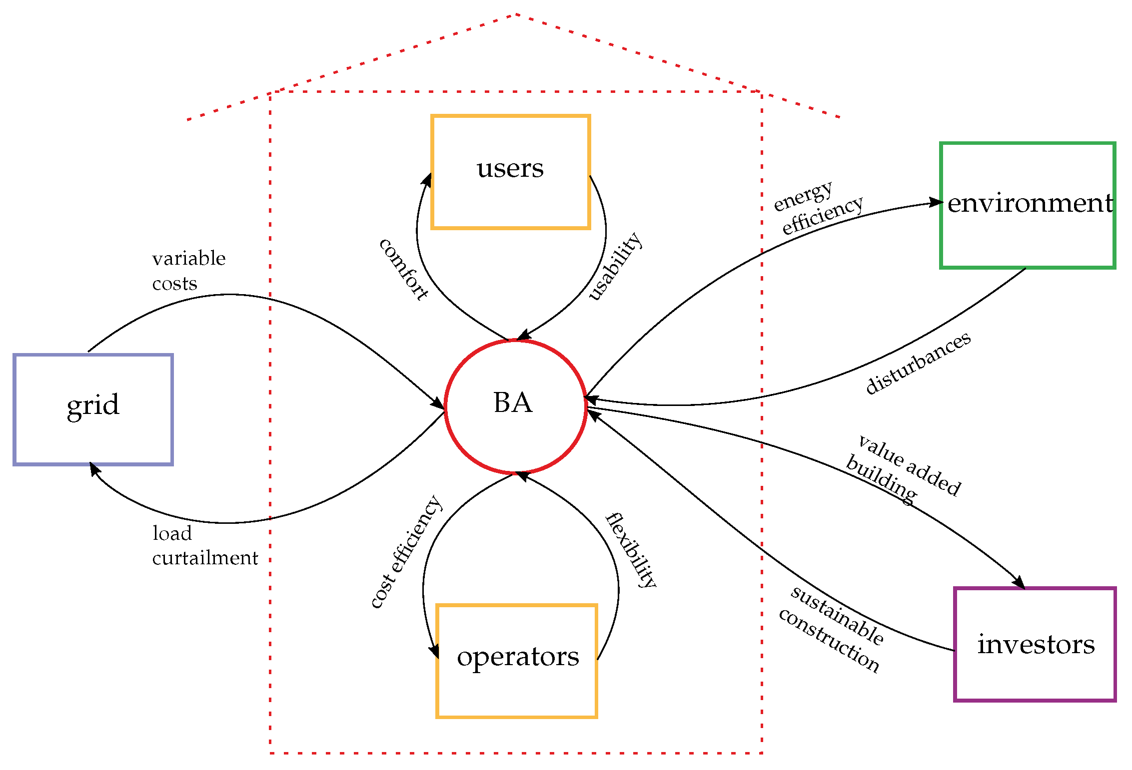
2.1. Building Automation and Sustainability

In [5], sustainability indicators for buildings are presented with the following key issues: resources consumption, environmental pressure, energy and water efficiency, indoor air quality, comfort and life cycle costs. Building automation affects sustainability in various manners influencing all of these indicators directly or indirectly in the building operation phase. Therefore, the performance of the overall building automation system becomes important for users, operators and the power grids. The demands of each group affect sustainable building automation. Sustainability for users means a high level of thermal comfort with the opportunity to adjust certain comfort parameters by themselves [11]. Operators are interested in a reduction of costs, including life cycle costs due to maintenance. Furthermore, the expected life cycle of a building is exceptionally long, and the objective of building operation might change from cradle to grave. Thus, flexibility and an intuitive interaction with the system is required from the building automation. Flexibility is also a key factor for the interaction with smart grids. Smart grids demand smart buildings with the capability of dealing with varying prices, demand response and load curtailment [12]. In return, they offer the advantage of temporarily low prices, which are again beneficial for operational cost efficiency. Within the building operation phase, cost efficiency goes along with energy efficiency if the potential for the usage of renewable energy sources can be realized. Thus, the usage of fossil fuels can be minimized, positively affecting the environmental pressure. Finally, investors are indirectly interested in sustainable building automation since they can expect an added value of the building as long as they provide a sustainable construction with infrastructure, such as free cooling or a geothermal source. Figure 1 shows the interaction of building automation with the most affected groups and the environment.

Model predictive control (MPC) as introduced in Section 2.2 is a powerful tool for sustainable building automation since the following requirements can be met:

• sustainable user satisfaction, including thermal comfort and usability.
• energy efficiency, including a maximal usage of renewable energy sources.
• minimization of costs, including life cycle costs arising due to the minimization of aggregates’ wear.
• flexibility towards smart grids by taking advantage of varying prices and fulfilling load curtailment.

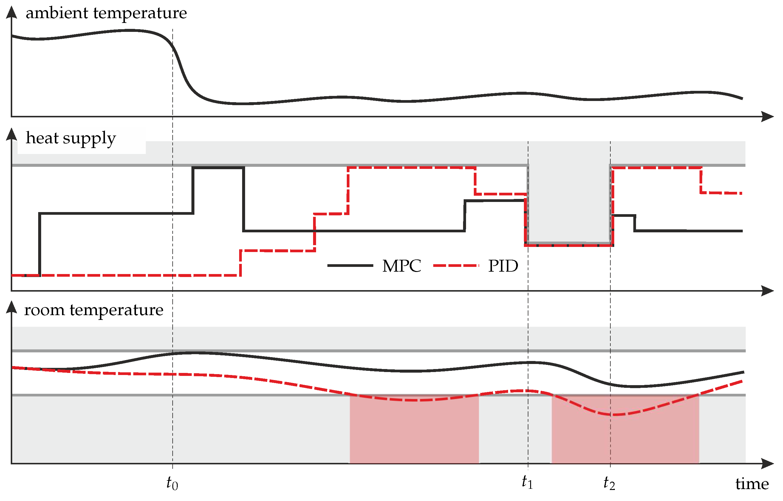
This paper focuses on non-residential buildings, which significantly differ from residential ones concerning the extent of building automation. However, the methodology of MPC is applicable also for residential buildings.

2.2. MPC versus PID

Model predictive control (MPC) is a standard method from advanced process control; it is based on a dynamic process model, predictions of disturbances, set-points and constraints and an optimality criterion. The manipulated variables (process inputs) are optimized such that contradicting goals, such as minimal control error and minimal control effort, are met in a suitable compromise. This optimization is performed by repeated on-line simulation of the process, its disturbances and the candidate input values to be optimized. As a result, the optimal process inputs fully respect time-varying constraints and the dynamic behavior of the process.

These features are illustrated for building automation in Figure 2.

In the upper plot, the ambient temperature (main disturbance) is shown. At $t=t_0$, a sudden drop in the ambient temperature occurs. The middle plot shows the heating input to the building. Two inputs from alternative control concepts are shown: PID (red, dashed) and MPC (black, continuous). Note that between $t=t_1$ and $t=t_2$, a strong constraint on the available heat input is active (e.g., caused by a grid overload). The bottom plot shows the mean temperature in the building together with an acceptable comfort band (between shaded areas).

Since MPC considers both the building’s time constants, the future disturbances and future constraints, it can pre-heat the building before the problem actually occurs. Since constraints are incorporated in the optimization, both input and comfort constraints are met. PID control reacts only to the increasing control error, thus violations of the lower temperature constraints occur (see the red regions in the bottom plot).

2.3. MPC Approaches in Building Automation

In recent years, several different approaches for the application of MPC in building automation have been presented [13]. Their key differentiators are the overall control structure, the type of MPC, the underlying building model and the application. Most of the concepts consider either the user level or the energy supply level. For the control of a multi-zone user level, centralized [9], decentralized, distributed [14] or cooperative configurations [15] have been proposed in the literature. The centralized controller delivers one solution for all zones, but the optimization results in a high computational load, since it incorporates the inputs, outputs and disturbances for all zones. Solving the control task for each zone separately in several decentralized MPCs reduces the computational burden. However, decentralized MPCs are not capable of taking coupling instances into account, a drawback that can be overcome by distributed and cooperative MPC schemes by sharing information between the MPCs in a cooperative loop. In [10], a hierarchical structure was chosen where the MPC determines the set-points for the low-level PID controller, but does not affect the energy supply system.

The type of MPC used depends on the type of system model. Buildings’ heating, ventilation and air conditioning (HVAC), as well as energy supply behavior are strongly non-linear systems. Modeling is a crucial part for MPC in buildings [16], since models are expected to be as accurate and yet as simple as possible. Hence, approximation is welcome as long as model validation assures acceptable error. For the user level, models have been identified using either statistical methods [16], physical modeling [10] or black-box identification routines [17].

MPCs for cooling or heating supply systems have been presented in, e.g., [18] based on non-linear and in [19] or [20] on hybrid system models. The energy supply level is mostly modeled based on non-linear differential equations, such as energy balance equations. Most of the MPCs are deterministic, meaning that the forecast for uncertain disturbances is used as known input. However, stochastic MPCs have been proposed for problem formulations involving uncertainties [21]. Furthermore, MPC approaches have been presented for the interaction with smart grids [12,22], as well as MPC usage for the optimization of power grids [23].

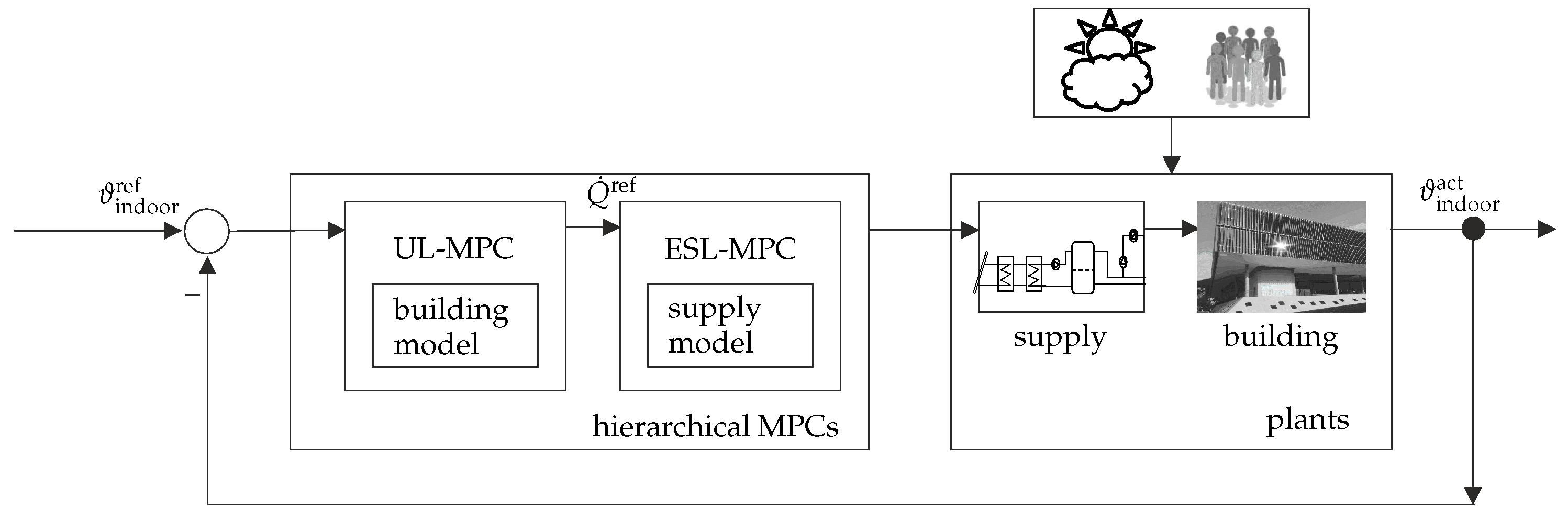
3. Hierarchical Model Predictive Control

In this section, the proposed HMPC is introduced based on the example of a demonstration building representing a large modern office building. However, due to its modularity, the control concept presented in Section 3.1 is also applicable to other buildings. In Section 3.2 and Section 3.3, the user level MPC and the energy supply level MPC are presented.

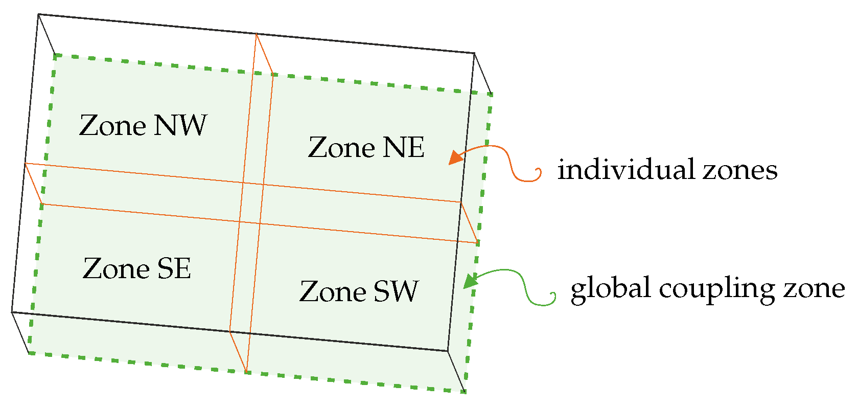
3.1. Hierarchical MPC Concept

A HMPC structure facilitates the flexibility to meet the requirements defined in Section 2.1. Two separately operating MPCs are independently designed, implemented and tuned and thus ideal for retrofit application, as well as for new buildings. The hierarchy splits the buildings into two layers, the user level and the energy supply level. Concerning control, the characteristics of these two layers differ significantly in their objective, the influencing disturbances and the system dynamics. The MPC on the user level, optimizing user comfort and minimizing heating/cooling energy, incorporates ambient temperature, radiance and the occupancy profile as disturbances. The system dynamics are basically slow since the thermal inertia of the building leads to time constants of several hours up to two days. The MPC on the energy supply level, supplying the necessary heating/cooling energy for the user level while fulfilling other conflicting goals, such as minimal costs, maximum usage of renewables and minimum wear, is affected as well by the ambient temperature and the water return temperatures of the building. The system dynamics are much faster than those of the user level. Furthermore, the HMPC is also an enabler for the interaction with a smart grid, since the two MPCs are flexible regarding varying prices and constraints possibly active due to load curtailment. The overall control structure is given in Figure 3.

The two MPCs are hierarchically operating, meaning that the optimized energy demand trajectory generated by the user level MPC ${\dot{Q}}^{\mathrm{ref}}$ is reference for the energy supply level MPC. Hence, $\dot{Q}$ is the only coupling point.

3.2. User Level MPC

The user level MPC is employed for optimizing the user comfort and minimizing the heating and cooling energy. Since this goal can be achieved by using the orientation specific radiance and the building as passive storage, the building is divided into independently controllable zones with different orientation; see Figure 4.

The MPC is then responsible for keeping the mean zone temperature within a predefined comfort band, taking the forecasts of the main disturbances of ambient temperature, radiance and the occupancy profile into account. While some heating or cooling systems provide energy for each zone individually, some HVAC systems supply the entire floor affecting the comfort parameter of all zones. Thus, these systems, such as ventilation systems or thermally-activated building systems (TABS), are coupling variables for all zones. In this paper, two supply systems are respected: the fan coil (FC) system supplying each zone individually and a common TABS providing all zones with heating or cooling energy. Different MPC approaches for the user level have been presented in the literature; cf. Section 2.3. However, for this study, a cooperative fuzzy MPC scheme (CFMPC) [15] is chosen, since it is most appropriate for the specific system identification approach. Depending on the seasons (winter, summer, transition), three local linear models (LLMs) are approximately characterizing the non-linearity of each zone. Note that depending on the local climate, the optimal number of LLMs can vary for a specific building. The fuzzy MPCs (FMPC) are implemented consisting of one linear MPC for each LLM, calculating the resulting control variable and the corresponding manipulated variables by applying fuzzy rules. The overall CFMPC thus includes one fuzzy MPC for each zone cooperatively acting with one global MPC for the coupling TABS control. Cooperation in this case means that two controllers, one respective FMPC of zone i and the global MPC, have to agree on one solution that is acceptable for both. This is done between all four FMPCs and the global MPC by an iterative loop with the aim that the corresponding manipulated variables converge to an optimum. Note that this approach enables flexible integration of new zones, as well as additional controlled variables: All existing MPCs can be retained without adjustments, and just the MPCs for the new parts have to be integrated in the cooperation loop.

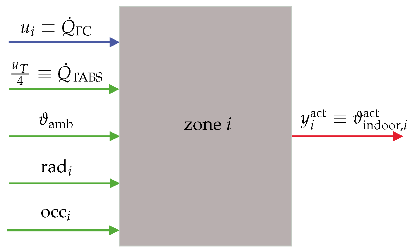
3.2.1. Building Model

Modeling is the most time-consuming part designing a model predictive controller. Since buildings are complex processes with non-linear system dynamics, modeling is especially demanding in this field.

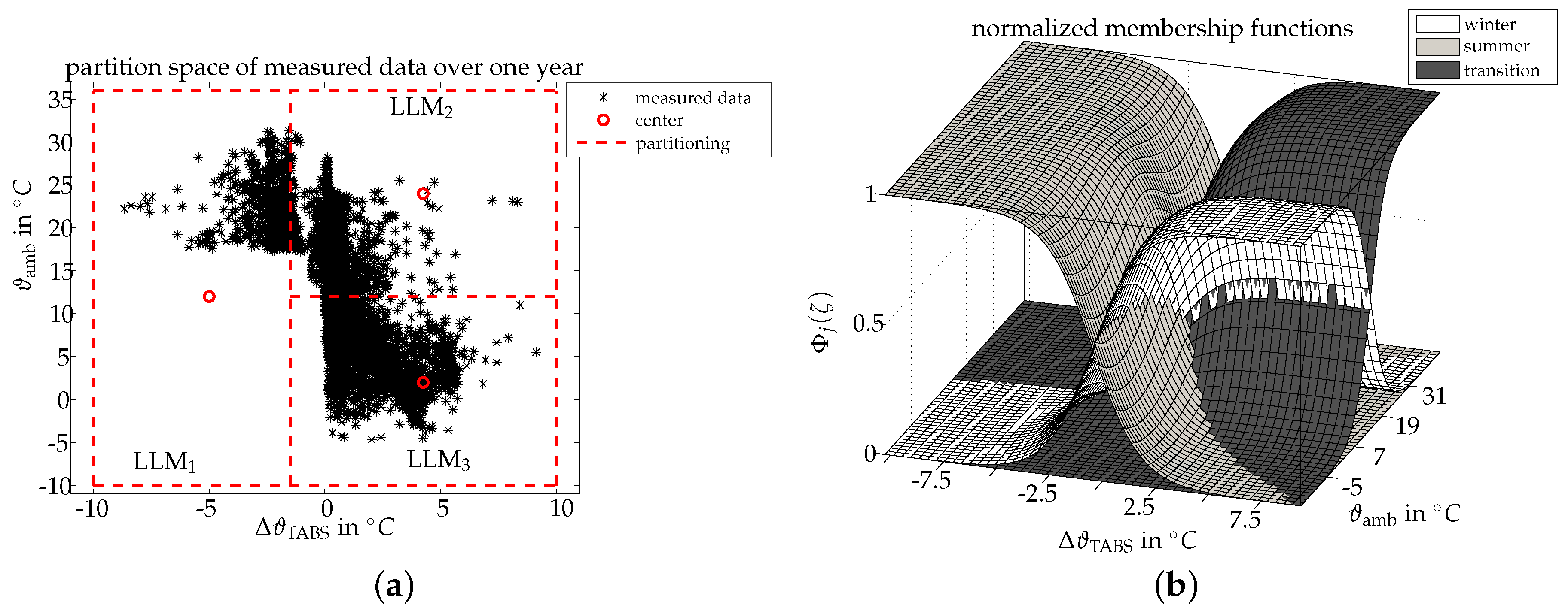
TS-Fuzzy Building Model

Four zones of the data-driven building model have the structure of a Takagi–Sugeno (TS)-fuzzy model. TS-fuzzy models are suitable to approximate nonlinear systems by interpolating between local linear, time-invariant autoregressive models with exogenous inputs (ARX) [24]. The basic element of a TS-fuzzy system is a set of fuzzy inference rules ${\mathbf{R}}^j$ [25]. In the following, $\zeta =\left[{\zeta }_1,\dots ,{\zeta }_p\right]\in {\mathbb{R}}^p$ is the vector of partition variables, and ${\Xi }_{j,1},\dots ,{\Xi }_{j,p}$ are the fuzzy sets or regions for the j-th rule ${\mathbf{R}}^j$ with corresponding membership functions ${\mu }_{j,{\Xi }_1},\dots ,{\mu }_{j,{\Xi }_p}$, with ${\mu }_{j,{\Xi }_i}\left({\zeta }_i\right)\mapsto \left[0,1\right]$, for $i=1,\dots ,p$ [17]. The number of rules $r_i$ in this work is the same as the number of local linear models (LLMs) $L_i$, $\forall i\in \mathbb{F}$ [17].

The elements of the fuzzy vector are usually a subset of the past input and outputs [24]. TS-fuzzy models consist of both fuzzy inference rules and local analytic linear dynamic models as follows,

$$\begin{array}{ccc}\hfill {\mathbf{R}}^j:& \mathrm{IF}& {\zeta }_1\mathrm{is}{F}_1^j\mathrm{and}\dots {\zeta }_p\mathrm{is}{F}_1^p\hfill \\ & \mathrm{THEN}& x^{k+1}=A_j^k{x}^k+B_j^k{u}^k\hfill \\ & & y^k=C_j^k{x}^k,\hfill \end{array}$$

(1)

where $j\in L=\{1,\dots ,p\}$ denotes the number of LLMs (rules).

The degree of fulfillment of the specific j-th rule can be computed using the product operator ${\mu }_j\left(\zeta \right)={\prod }_{i=1}^p{\mu }_{j,{\Xi }_i}\left({\zeta }_i\right)$; furthermore, the normalized degree of fulfillment can be computed as:

$${\mathrm{\Phi }}_j\left(\zeta \right)=\frac{{\mu }_j\left(\zeta \right)}{{\sum }_{l=1}^L{\mu }_l\left(\zeta \right)}.$$

(2)

The overall zone model is given as a superposition of the above defined local linear models. This superposition is achieved by weighted parameter blending of the individual system matrices over all LLMs:

$$A^k=\sum _{j=1}^L{\mathrm{\Phi }}_j\left(\zeta \right)A_j^k,B^k=\sum _{j=1}^L{\mathrm{\Phi }}_j\left(\zeta \right)B_j^k,C^k=\sum _{j=1}^L{\mathrm{\Phi }}_j\left(\zeta \right)C_j^k$$

(3)

Each zone model of the building can thus be formally written as a time-varying linear state-space system:

$$\begin{array}{cc}\hfill x^{k+1}=& A^k{x}^k+B^k{u}^k\hfill \\ \hfill y^k=& C^k{x}^k.\hfill \end{array}$$

(4)

The global coupling zone (see Figure 4) can be modeled by a linear time-invariant state-space system represented by the matrices $A_g$, $B_g$ and $C_g$.

Note that four building zones plus the linear coupling zone have been considered, and each TS-fuzzy zone model consists of three LLMs. Each TS-fuzzy model has five inputs and the mean room temperature of the respective zone as the output (see Figure 5).

Specific Building Model

For each zone of the specific building, the significant nonlinearities are given by a two-dimensional partition space spanned by the difference between heat supply and return temperatures of the manipulated variable TABS (denoted by $\Delta {\vartheta }_{\mathrm{TABS}}=({\vartheta }_{{\mathrm{TABS}}_{\mathrm{supply}}}-{\vartheta }_{{\mathrm{TABS}}_{\mathrm{return}}})$) and the ambient temperature (denoted by ${\vartheta }_{\mathrm{amb}}$). Both the choice of the partition variables and the model split have been done by expert knowledge; however, they could also be identified by a local linear model tree algorithm (LoLiMoT) [17]. In any case, after partitioning of the measured data, classical linear identification methods like least squares can be utilized to estimate the matrices of the individual LLMs (1).

The LLMs and the specific partition space for the building are presented in Figure 6a. Note that in this building, the partition space with the model splits is identical for all zones. For more detailed information and extensive model validation, see [15,26]. It is shown there that all TS-fuzzy zone models achieve $R^2$-values above 0.9 for three or more LLMs.

3.2.2. Objective

The objective of the user level MPC, for each FMPC of zone $i\in \{1,...,4\}$, is to maximize the user comfort and to minimize the energy demand. The resulting trade off is mathematically expressed by the quadratic objective function given in (6).

$$J_i^{\star }=\underset{u_i}{min}{J}_i\left(u_i\right)$$

(5)

$$J_i=\alpha \sum _{k=0}^{Np}{(y_i^{\mathrm{ref}}\left(k\right)-y_i^{\mathrm{act}}\left(k\right))}^{\prime }{Q}_i(y_i^{\mathrm{ref}}\left(k\right)-y_i^{\mathrm{act}}\left(k\right))+(1-\alpha )\sum _{k=0}^{Np}{u}_i^{\prime }\left(k\right)R_i{u}_i\left(k\right)$$

(6)

The control variable $y_i^{\mathrm{act}}$ denotes the actual mean zone temperature for the i-th FMPC and $y_i^{\mathrm{ref}}$ its reference value. The vector $u_i$ represents the energy demand to be optimized for the FC system, the TABS and the given disturbances radiance and ambient temperature for zone i. The i-th FMPC calculates an optimized strategy looking $Np$ steps ahead by minimizing the sum of the costs arising due to the deviation and the energy demand penalized with the time-invariant penalty matrices $Q_i$ and $R_i$, respectively, each time step k. The optimization problem is subject to the constraints in (7) and the usage of the model introduced in the previous section. The parameter $\alpha \in [0,1]$ is free to be chosen by the operator in order to put either more weight on the minimization of the deviation of the user comfort parameter or on the minimization of the energy demand.

$$\begin{array}{cc}\hfill u_{i,\min }& \le u_i\le u_{i,\max }\hfill \\ \hfill y_{i,\min }& \le y_i^{\mathrm{act}}\le y_{i,\max }\hfill \end{array}$$

(7)

The constraints guarantee that the optimized energy demand is kept within technically feasible limits and that the mean zone temperature does not violate a predefined comfort band. The MPC solves the corresponding optimization problem each time step k. Though the optimal strategies $U_{i,\mathrm{FC}}^{\star }$ for FC and $U_{\mathrm{TABS}}^{\star }$ for TABS are computed for the entire prediction horizon $Np$, only the first elements $u_{i,\mathrm{FC}}^{\star }\left(k\right)$ and $u_{\mathrm{TABS}}^{\star }\left(k\right)$ are applied to the system, and at the next time instance, the optimization is repeated with the updated disturbances yielding a receding horizon strategy. Since the objective in (6) is a quadratic function and constraints of the form (7) have to be respected, a solver has to be chosen that is capable of solving a constrained quadratic program. For this study Matlabsolvers have been used https://de.mathworks.com/help/optim/ug/quadratic-programming-algorithms.html.

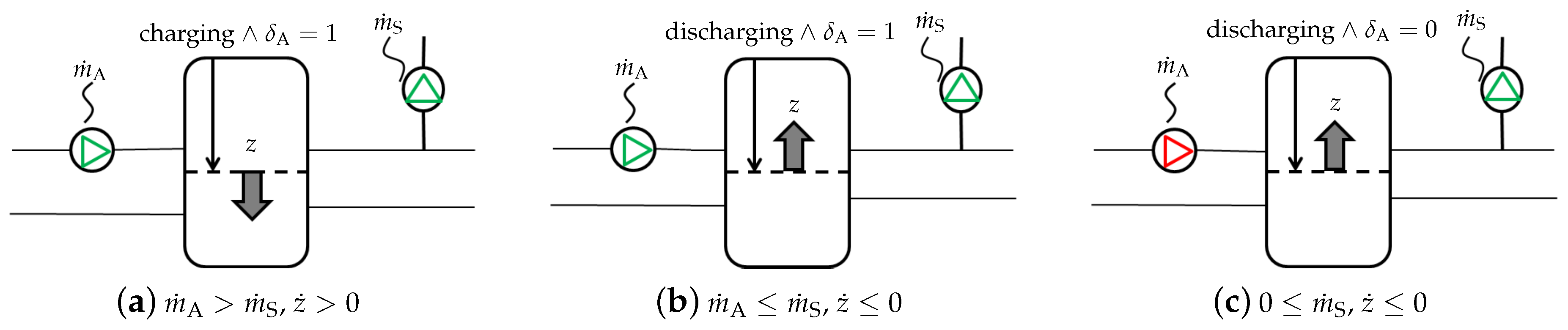
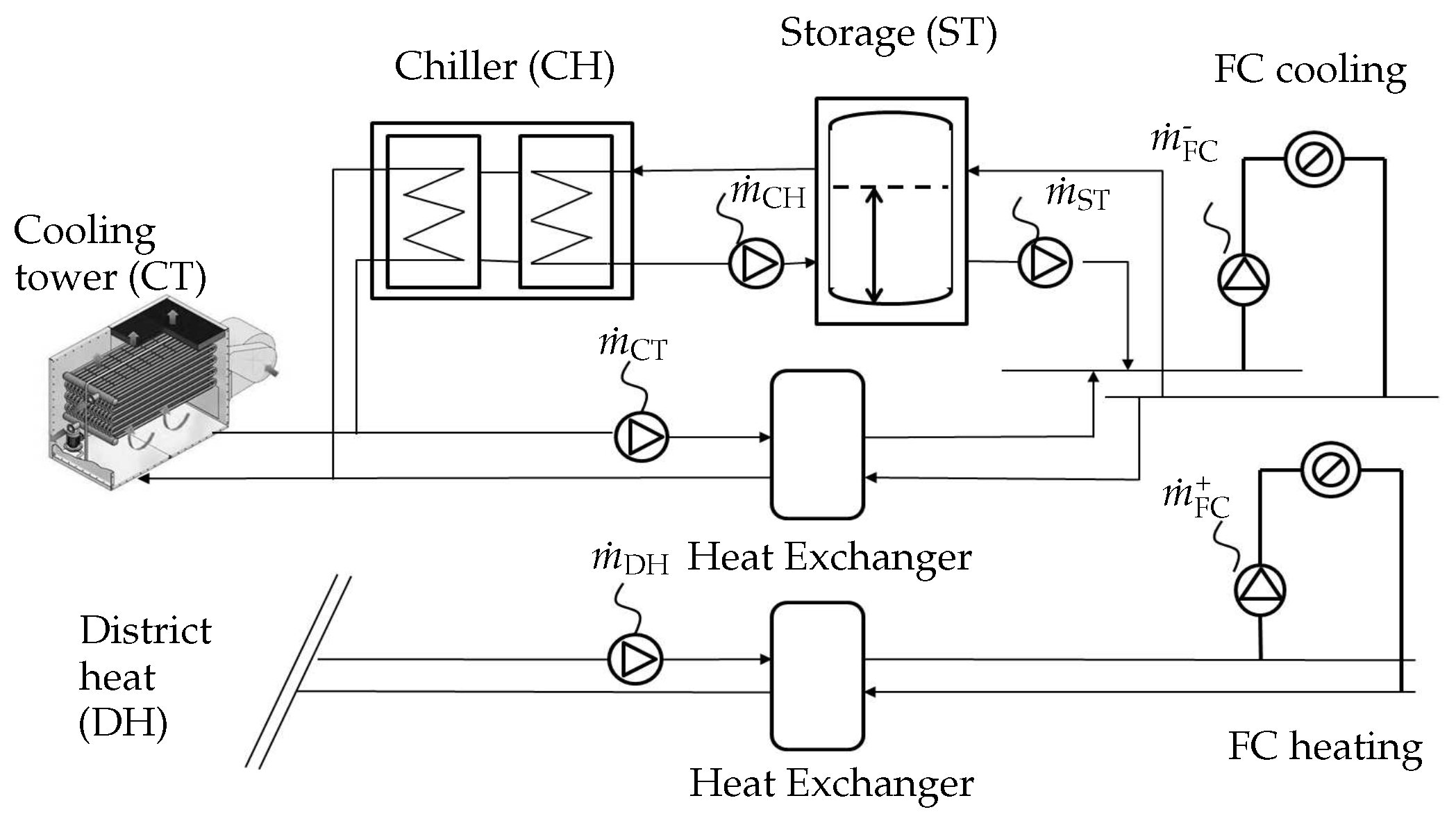
3.3. Energy Supply Level MPC

The energy supply level MPC is responsible for minimizing the energy costs, to maximize the usage of renewable energy sources while delivering the energy demand of the user level accurately. The energy supply level consists of several supply circuits routed from various energy sources to the supply systems incorporating heat exchangers, aggregates and water storage tanks. Figure 7 illustrates such circuits exemplarily for the fan coil (FC) supply, including free cooling, the chiller and subsequent stratified water storage tank for cooling and district heat supply for heating.

The proposed MPC for this level is a modular predictive control concept (MPCC) including a mixed-integer MPC (MI-MPC) [27]. This special MPC has not only all of the advantages presented in Section 2.1, but is also capable of optimizing discrete and continuous variables at the same time. This becomes necessary if the underlying system contains switching instances, such as chillers, which influence the operation mode of the subsequent storage in a discontinuous fashion. With this type of MPC, the number of transitions of the aggregates from the state off to on can be reduced significantly [28], leading to less life cycle costs due to minimal wear. The MPCC includes one MPC for each circuit, depending on the respective building’s physical structure. If supply systems are connected with circuits provided by fossil fuels, as well as by renewable energy sources, the MPCC always prefers the circuits with renewables. Given the example in Figure 7, cooling energy for FC is supplied by free cooling as long as all technical conditions such as the ambient temperature limit are fulfilled.

3.3.1. Energy Supply Model

Modeling the energy supply system for the proposed MPCC is done based on thermodynamic principles [18,20]. Circuits with heat exchangers only are treated as linear systems, approximated by linearized first order differential energy balance equations. Circuits with additional aggregates and storage are seen as hybrid systems, since the state of the aggregate ${\delta }_A$ affects the operation mode of the storage, such that one model is required for each mode. The resulting model is a nonlinear piecewise affine system of the following form:

$$x(t+1)=\left\{\begin{array}{cc}{A}_{1}x\left(t\right)+B_{1}u\left(t\right),\hfill & \mathrm{if}{\delta }_1\left(t\right)=1\hfill \\ A_{2}x\left(t\right)+B_{2}u\left(t\right),\hfill & \mathrm{if}{\delta }_2\left(t\right)=1\hfill \\ A_{3}x\left(t\right)+B_{3}u\left(t\right),\hfill & \mathrm{if}{\delta }_3\left(t\right)=1,\hfill \end{array}\right.y(t+1)=\left\{\begin{array}{cc}{C}_{1}x\left(t\right)+D_{1}u\left(t\right),\hfill & \mathrm{if}{\delta }_1\left(t\right)=1\hfill \\ C_{2}x\left(t\right)+D_{2}u\left(t\right),\hfill & \mathrm{if}{\delta }_2\left(t\right)=1\hfill \\ C_{3}x\left(t\right)+D_{3}u\left(t\right),\hfill & \mathrm{if}{\delta }_3\left(t\right)=1,\hfill \end{array}\right.$$

(8)

with ${\delta }_1\iff \mathrm{charging}$ ∧ ${\delta }_{\mathrm{A}}=1$, ${\delta }_2\iff \mathrm{discharging}$ ∧ ${\delta }_{\mathrm{A}}=1$ and ${\delta }_3\iff \mathrm{discharging}$ ∧ ${\delta }_{\mathrm{A}}=0$. Figure 8 illustrates the three basic modes: charging, discharging if the aggregate is active and discharging if the aggregate is inactive.

For detailed information about the modeling, see [20], and for model validation, the reader is referred to [28].

3.3.2. Objective

For the MPC implementation, a quadratic optimization target is used, where the deviation to the reference trajectory of the cooling respective heating power is penalized with factor S. Furthermore, the energy costs represented by $T_k$, caused by the manipulated variables (mass flows of the pumps) are taken into account. Note that the penalty matrix T depends on the time instance k, meaning that varying prices can be respected. Both additive terms are considered for each time step k over the whole prediction horizon $Np$. The parameter α is again a weighting factor, which can be modified easily by the operator in order to shift the importance between the accuracy of the delivered power and the energy costs. The formal description of the objective is given by:

$$\begin{array}{c}\hfill J^{\star }=\underset{u\in U}{min}\left[\alpha \sum _{k=0}^{Np}{({\dot{Q}}_j^{\mathrm{ref}}\left(k\right)-{\dot{Q}}_j^{\mathrm{act}}\left(k\right))}^{\prime }S({\dot{Q}}_j^{\mathrm{ref}}\left(k\right)-{\dot{Q}}_j^{\mathrm{act}}\left(k\right))+(1-\alpha )\sum _{k=0}^{Np}{u}^{\prime }\left(k\right)T_{k}u\left(k\right)\right],\end{array}$$

(9)

where $j\in \{\mathrm{FC},\mathrm{TABS}\}$ determines the supply system, and the vector $u_j$ represents the manipulated variables, such as mass flows and supply temperatures to be optimized for the supply of the FC system and the TABS.

$$\begin{array}{cc}\hfill u_{j,\min }& \le u_j\le u_{j,\max }\hfill \\ \hfill x_{j,\min }& \le x_j\le x_{j,\max }\hfill \end{array}$$

(10)

The optimization problem with the target given in (9), the hybrid model introduced in (8), with constraints on the manipulated variables, and the states given in (10) result in a mixed-integer quadratic problem, which can either be solved by commercial solvers, such as [29], or approximated by, e.g., branch and bound algorithms, such as introduced in [28].

Note that the prediction horizon $Np$ for the energy supply level MPC is shorter than the one for the user level MPC (6 h versus 25 h) since the time constants are much smaller in the energy supply level.

4. Simulation Results

The performance of the HMPC for sustainable building automation is demonstrated based on the example of a large office building in Salzburg, Austria. The description of the demonstration building is given including the currently active PID control structure and the HMPC integration in the building automation system (BAS) before the simulation results are shown regarding the requirements set up in Section 2.1. All building and energy supply models have been identified, respectively implemented in Matlab. The HMPC implementation, as well as the simulation have also been conducted in Matlab.

4.1. Demonstration Building

The demonstration building for this study is a 27,000 m${}^2$ University building in the center of Salzburg, Austria. It has five floors above ground containing several large and numerous smaller meeting rooms, offices and lecture rooms. For this work, focus is put on the second and third floor, which is comprised of about 500 rooms of some 13,000 m${}^2$, almost all used as offices. Both floors are supplied by fan coils (FC) and a thermally-activated building system (TABS) coupling the four zones; see Figure 4. The energy supply system of this building consists of heating and cooling supply circuits for FC (see Figure 7) and TABS. The FC system is provided energy from district heat and cooling energy from free cooling or the chiller, whereas the geothermal source supplies the TABS including a heat pump in the case of heating. The results presented in the following sections are based on simulation results, but the HMPC concept is already in the test phase implemented in the demonstration building’s automation system. The simulation is shown for representative snapshots of the three seasons: transition periods (13 April–12 May 2014 and 16 October–15 November 2014), summer (4 July–11 August 2014) and winter (19 January–28 February 2015). The corresponding historic data for disturbances and comparison analysis are taken from the implemented building automation system.

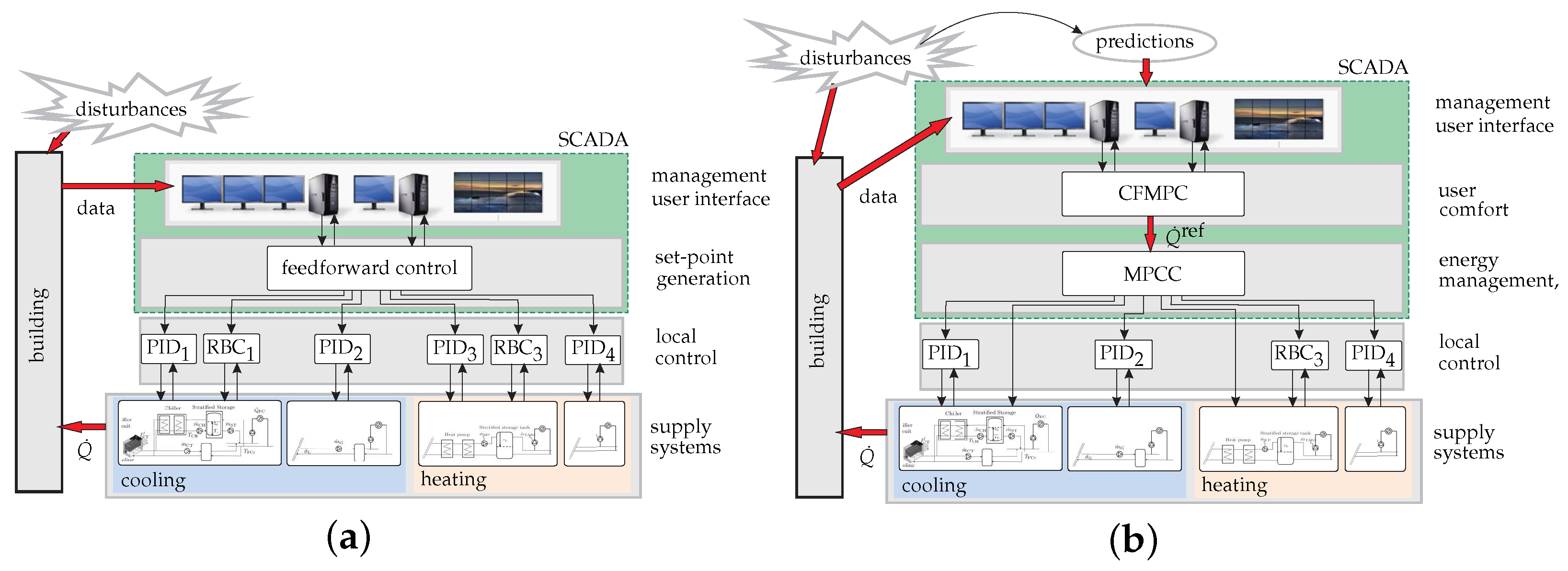
4.1.1. State-Of-The-Art PID Control Structure

The state-of-the-art PID-control structure designed for and currently active in the demonstration building consists of PIDs together with RBC loops. In the user level PID control, the room temperatures are based on the comfort requirements of the users. In the energy supply level, all supply temperatures are controlled by individual PIDs. The set-points are calculated in the PLCby comparing the recent past of the ambient temperature to a predefined skid. The mass flows of the corresponding supply pumps are kept constant. Switching on and off the heat pump, respectively the chiller, is decided in an RBC loop where fixed temperature limits of the stratified storage tanks are respected. Figure 9 shows the PID controllers and RBC loops within the overall building automation system.

4.1.2. HMPC Integration in the Building Automation System

The implementation of the proposed structure in existing building automation systems (BAS) is straightforward. Basically, it can be seen as part of an extended supervisory control and data acquisition (SCADA) system. As shown in Figure 9, the conventional function of (mainly feedforward) set-point generation for the underlying PID and RBC loops is replaced by the proposed hierarchical structure. The MPCC replaces some of the local control loops; nevertheless, in most cases, the existing local control loops with their respective safety functions can be utilized. Note that disturbances (weather and occupancy) are explicitly considered by predictions.

Both CFMPC and MPCC can be directly integrated in the SCADA system, as the functions of a flexible programming structure are given in the BAS. Another solution is possible by setting up a dedicated hardware and software for the predictive controllers, which communicate by standard interfaces with the SCADA system and local controllers.

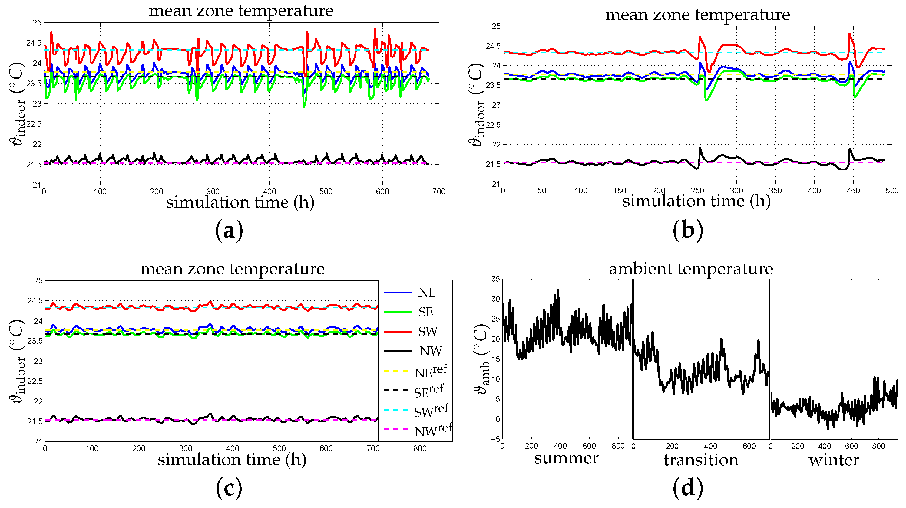
4.2. User Satisfaction

User satisfaction in terms of sustainable building automation primarily means fulfillment of user comfort requirements. The user level MPC, here represented by the CFMPC, is capable of predicting the energy needed for the individual zones in order to keep the respective mean zone temperature not only within the comfort band, but around a predefined reference value. The comfort band for this simulation has been chosen with a tolerance of $\pm 2{}^{\circ }$C of the reference value individually for each zone. Figure 10a–c shows the simulation results for the three seasons.

The plots show the reference, as well as the mean zone temperature for the four zones respectively. For all periods, the thermal comfort is guaranteed with little deviation to the constant reference value and, thus, all times within the comfort band. One can see a higher frequency in summer arising due to the higher amplitude of the radiation in summer compared to the other periods. Figure 10d shows the ambient temperature for the respective season. All disturbances are taken from snapshots of the Central Institute for Meteorology and Geodynamics in Salzburg, ZAMG. The occupancy profile is generated generically as in [15] according to the occupancy pattern for offices adapted from [30].

User satisfaction is also affected by the degree of individual control of users’ respective operators. Therefore, the automation system has to enable an easy and intuitive adjustment of optimization settings. One of these parameters is $\alpha \in [0,1]$ representing how much emphasis is either put on the thermal comfort satisfaction or on the cost minimization in the energy supply level MPC’s objective. In order to demonstrate the consequence of the variation, simulation runs are conducted with α varying from 0.1–0.9. The results are given in

Table 1. Simulation results in terms of costs and MAE (kW) for varying weighting parameter α.

$\mathbf{\alpha }$	Summer		Transition		Winter
	Costs $\mathbf{\left(}{\mathbf{10}}^{\mathbf{6}}\mathbf{\right)}$	MAE	Costs $\mathbf{\left(}{\mathbf{10}}^{\mathbf{6}}\mathbf{\right)}$	MAE	Costs $\mathbf{\left(}{\mathbf{10}}^{\mathbf{6}}\mathbf{\right)}$	MAE
0.1	4.4253	2.28	1.63540	0.26	2.0305	0.014
0.5	4.4266	2.27	1.63542	0.25	2.0302	0.002
0.9	4.4267	2.26	1.63929	0.22	2.0340	0.000

in terms of resulting quadratic costs and the mean absolute error (MAE) of the MPC output to the reference value for the three seasons. The building requires on average about 550 kW of cooling power in summer and 750 kW of heating power in winter. The higher α, the higher the (energy) costs and the less the error of the energy supply to the energy demand of the user level. Note that in winter, the error is generally much smaller since the energy demand from the user level is less volatile. For an industrial application, a cost reduction is preferable, leading to a small α, which can be recommended in this case since the MAE does not vary a lot. Note that the energy costs are calculated by considering the electric effort of all pumps according to their characteristic curves, as well as the chiller with a coefficient of performance of 3.9. For more details, see [28].

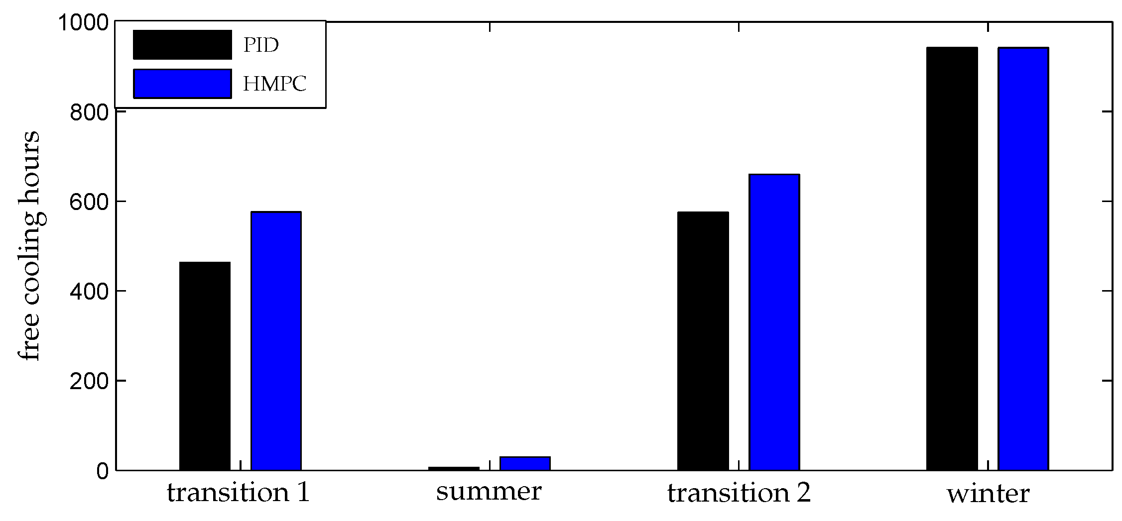
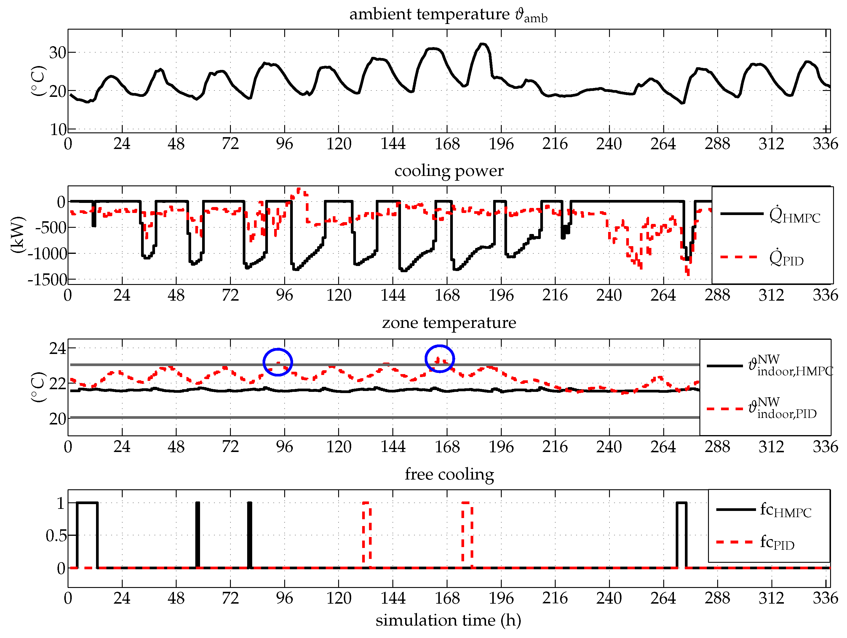
4.3. Energy Efficiency

The HMPC enables an energy-efficient building operation due to the minimization of energy demand in the user level and due to maximal usage of renewable energy sources in the energy supply level. Free cooling is the representative renewable source for this study addressable in the demonstration building. Figure 11 shows the active free cooling hours according to the strategy of the HMPC and the currently-implemented PID controller in the building for spring (transition 1), summer, autumn (transition 2) and winter.

The results show a big potential for the transition period, as well as summer, since the MPCC is capable of predicting time slots of ambient temperature below the technical limit, whereas the PID controller only reacts on weather data from the past. For the entire simulation period, an additional 221 active free cooling hours have been achieved, which means an overall increase of 11%. However, for the transition periods, up to 25% more free cooling hours become feasible with the HMPC. Note that the high amount of cooling hours in winter is a result of continuous cooling of the server rooms. The total number of cooling hours in summer is 694 with the MPCC or 684 with the PID control. Further simulation results have been presented in [28], where additionally explicit costs and the cooling energy provided by free cooling are compared, resulting in about 50% less electric energy costs for cooling and the double amount of cooling energy supplied via free cooling for the transition month of May.

Figure 12 shows the difference between the control strategy of the PID/RBC structure and the proposed HMPC concept. All data concerning the PID/RBC results are taken from the demonstration building’s BAS database. The first subplot shows the ambient temperature. Note that the days are often quite hot, and the nights remain chilly, which can be considered as a sudden drop concerning the time constants of the building, such as demonstrated in Figure 2. The second subplot shows the differences of the cooling supply strategy. The HMPC pre-cools the building during night where the electric energy is less expensive, whereas the PID structure reacts if the ambient temperature gets hotter for some hours. The third subplot shows the resulting indoor zone temperature. Note that the HMPC can keep the temperature in the comfort band (marked with the gray lines) over the entire simulation period, but the PID sometimes violates it; see the blue marked spots. Furthermore, the HMPC reduces the variance significantly. The last subplot shows when the PID, respectively the HMPC, activates the supply via free cooling. At hours 130 and 173, the PID violates the rule that free cooling must not be activated if the ambient temperature is higher than 18 ${}^{\circ }$C, whereas the HMPC uses all possible periods for free cooling by meeting this requirement.

4.4. Life Cycle Costs

Life cycle assessment for buildings is generally a demanding task [2]. Nevertheless, reducing costs for energy supply systems in operation and maintenance is an effective means. Applying an MPC with the optimization target presented in Section 3.3.2 minimizes the wear of aggregates, such as chillers or heat pumps. For this simulation study, the number of transitions from state off to state on from the chiller is the reference measure. Figure 13 shows the simulation results compared to the measured transitions resulting from the PID control decision in the respective seasons.

The number of active chiller hours can be reduced by 206 h or 17%, and simultaneously, the number of transitions from state off to state on can be reduced by 11% or 35% with the MPCC for the entire simulation period. However, the results for individual seasons are much more promising, such as a reduction of chiller transitions of up to 50% in autumn and spring. Note that in winter, the chiller has not been active, since free cooling could be activated all of the time.

4.5. Flexibility towards the Smart Grid

Demand response programs vary in their price or incentive options, but in general, accepting load shift or curtailment is monetarily beneficial for building operators. For this simulation study, the winter period is considered. The exemplary price profile is based on fixed rates depending on the time of day; see Figure 14a. For the high-peak hours in the morning, at noon and in the evening, higher prices are accepted, but in turn, the price is lower (€1.0/kWh) than the constant price of €1.2/kWh for all other hours. The energy supply level MPC predictively incorporates the varying prices and optimizes the strategy such that more energy is demanded if the price is low and less if it is high. The resulting costs are therefore a little higher during the more expensive hours, but lower for the less expensive periods compared to the MPC results with a time-invariant price profile. Figure 14b shows a snapshot of the difference of the costs from the MPC simulations with a constant and a varying price profile, resulting in an overall cost reduction of 14% or €3.230 only for the heating TABS supply in winter. For the same high-peak hours, load curtailment is demanded at lower electricity costs. Figure 14c shows this requirement for the TABS supply represented by upper constraints in gray dashed lines. The user level MPC is capable of adjusting the strategy taking the load curtailment as a time variant input constraint into account (see the pink line), while still guaranteeing the desired user comfort over the entire simulation period; see Figure 14d.

5. Discussion

In this section, the results are discussed, and possible obstacles and necessary measures are given for the industrial usage of the proposed MPC concept.

5.1. Perspectives

In Section 2.1, Figure 1, the interaction of building automation with the most important groups is illustrated. In the following sections, the simulation results are discussed from the perspective of the buildings’ users, operators, investors and the smart grid.

5.1.1. User Perspective

Users judge the performance of building automation systems particularly in terms of thermal comfort. The simulation results in Section 4.2 show that a predictive control concept is capable of guaranteeing high user comfort with less energy demand. Even if load curtailment is accepted at some hours a day, the user comfort is kept within the predefined comfort band as illustrated in Section 4.5. Sustainability for users also means the opportunity to adjust certain comfort parameters by themselves. The objective function as a key element of MPCs is changeable within the building automation system. Thus, some tuning parameters can easily be disclosed for the users or operators. In Section 4.2, Table 1, the effect of changing the parameter α shows that the trade off between costs and thermal comfort can be regulated to some degree by the user. Note that different set-points for different zones are possible without compromising the overall optimum.

5.1.2. Operator Perspective

Operators are mainly interested in a reduction of costs, including life cycle costs. In Section 4.3, it is shown that the energy supply level MPC maximizes the usage of free cooling, which is in relation to other (fossil) sources a significantly less expensive solution. Thus, in building operation, energy efficiency is equivalent to cost efficiency. Regarding the life cycle costs the proposed energy supply level MPC reduces the aggregates’ wear and therefore maintenance effort by decreasing the aggregates’ transitions by 15%–50% compared to conventional PID control depending on the season. Additionally, the aggregates are less used if other (less expensive) sources are available. Thus, the chiller has 17% less active hours over the year. In Section 4.5, it is shown that the energy supply level MPC can additionally take advantage of varying prices by saving up to 10% for the chosen price profile.

5.1.3. Smart Grid Perspective

Smart grids demand smart buildings with the capability to deal with varying prices, demand response and load curtailment. The results in Section 4.5 clearly show that the HMPC concept meets these requirements and becomes therefore beneficial for a smart grid integration and simultaneously for a reduction of energy costs.

5.1.4. Investor Perspective

Providing sustainable construction with infrastructure, such as free cooling or geothermal source, is expensive. However, investors can expect a value added building if sustainable building automation is implemented, and a return on invest is possible since the infrastructure can be used efficiently. Moreover, the added flexibility of the proposed HMPC concept results in a robust building automation system, easily adaptable to future demands. It is thus also a contribution to risk mitigation.

5.2. Possible Obstacles and Necessary Measures

Several simulation studies [10,31], as well as the first prototypes of MPC implementations for large non-residential buildings [32] show the performance and the readiness level for industrial solutions of this intelligent control scheme. Nevertheless, some obstacles might complicate successful implementations and future market penetration. In the following sections, possible obstacles are addressed, and necessary measures are given.

5.2.1. Trained Personnel

An industrial usage of MPC as a key component in building automation requires the automation suppliers to employ experts in the field of building modeling and experienced control engineers for MPC design and implementation. The availability of competent and trained experts in this field may be the real bottleneck for market penetration. On the other side, also operating personnel are necessary who are willing to apply advanced control approaches not commonly used. For retrofitting projects, it has been proven advisable to involve operators early in the control design and implementation phase in order to integrate their knowledge of the process and the building’s specifics on the one side and to let them participate on the engineering progress to dismantle the fear from the new technique on the other side.

5.2.2. Data Acquisition

Building modeling is a crucial part for the MPC’s performance. Hence, for model identification, historic data from the building in operation are essential. The more powerful the automation system is regarding the data base structure, data acquisition and archiving, the better the basis for the resulting models. If input data or data from disturbances are missing or not appropriately assignable to its timestamps, the model quality may be poor. Therefore, the accessibility of sensors, as well as of, for instance, weather data from external systems is important.

5.2.3. Hardware Requirements

The proposed MPC approach works with existing building infrastructures for heating and cooling supply. However, the performance depends on the availability of information of the energy supply and building process. For the closed loop control of thermal comfort parameters, it is necessary to obtain actual measures of indoor room temperatures, energy supply to the respective zones, water supply and return temperatures, mass flows of pumps, etc. This requires the implementation, availability and integration of the corresponding sensors to the building automation system. In turn, all actuators, such as pumps or valves must be addressable in order to execute new set-points computed by the MPC.

6. Conclusions

The paper has presented a hierarchical model predictive controller (HMPC) for sustainable building automation. The proposed MPC structure sustainably affects the directly influenced groups, such as users, operators, investors, the environment or the power grid. The HMPC is capable of maximizing user comfort and the usage of renewable energy sources while minimizing energy demand and costs for buildings in operation. Additionally, it allows the integration of the resulting smart building in the smart grid. Furthermore, due to the HMPCs flexibility, changing legislative requirements can easily be applied with little investment, since only the optimization target of the HMPC has to be adapted. For example, a time-variant constant proportion of renewable energy sources can be guaranteed. The performance of the exemplarily proposed HMPC is demonstrated regarding the demands of the respective group by simulation results of a modern office building. For users, thermal comfort is guaranteed throughout all seasons, and the variation of a user-adjustable parameter shows the resulting trade off between user comfort and energy costs. Operators benefit monetarily from energy-efficient strategies and lower life cycle costs, since free cooling is used up to 25% more often than by the conventional PID controller instead of more expensive fossil sources. Furthermore, the aggregates’ wear is minimized due to a reduction of transitions from state off to on of up to 50%. Furthermore, an easy smart grid integration is possible, since the predictive character of the MPC is ideal to take advantage of flexible prices and to meet temporarily active load curtailment without violating the thermal comfort band. Finally, possible obstacles for a successful implementation of MPC in building automation are addressed, and necessary measures for a prosperous industrial development of MPC for sustainable building automation are given.

References

1. European Commission. “Buildings”. Available online: https://ec.europa.eu/energy/en/topics/energy-efficiency/buildings (accessed on 14 May 2016).
2. Khasreen, M.M.; Banfill, P.F.G.; Menzies, G.F. Life-Cycle Assessment and the Environmental Impact of Buildings: A Review. Sustainability 2009, 1, 674–701. [Google Scholar] [CrossRef] [Green Version]
3. Waddicor, D.A.; Fuentes, E.; Sisó, L.; Salom, J.; Favre, B.; Jiménez, C.; Azar, M. Climate change and building ageing impact on building energy performance and mitigation measures application: A case study in Turin, northern Italy. Build. Environ. 2016, 102, 13–25. [Google Scholar] [CrossRef]
4. Siano, P. Demand response and smart grids—A survey. Renew. Sustain. Energy Rev. 2014, 30, 461–478. [Google Scholar] [CrossRef]
5. Bragança, L.; Mateus, R.; Koukkari, H. Building Sustainability Assessment. Sustainability 2010, 2, 2010–2023. [Google Scholar] [CrossRef]
6. Dounis, A.I.; Caraiscos, C. Advanced control systems engineering for energy and comfort management in a building environment—A review. Renew. Sustain. Energy Rev. 2009, 13, 1246–1261. [Google Scholar] [CrossRef]
7. Maciejowski, J.M. Predictive Control: With Constraints; Pearson Education: Upper Saddle River, NJ, USA, 2002. [Google Scholar]
8. Camacho, E.F.; Alba, C.B. Model Predictive Control; Springer Science & Business Media: Berlin, Germany, 2013. [Google Scholar]
9. Oldewurtel, F.; Parisio, A.; Jones, C.N.; Gyalistras, D.; Gwerder, M.; Stauch, V.; Lehmann, B.; Morari, M. Use of model predictive control and weather forecasts for energy efficient building climate control. Energy Build. 2012, 45, 15–27. [Google Scholar] [CrossRef]
10. Širokỳ, J.; Oldewurtel, F.; Cigler, J.; Prívara, S. Experimental analysis of model predictive control for an energy efficient building heating system. Appl. Energy 2011, 88, 3079–3087. [Google Scholar] [CrossRef]
11. Shahzad, S.S.; Brennan, J.; Theodossopoulos, D.; Hughes, B.; Calautit, J.K. Building-Related Symptoms, Energy, and Thermal Control in the Workplace: Personal and Open Plan Offices. Sustainability 2016, 8, 331. [Google Scholar] [CrossRef]
12. Miletic, M.; Schirrer, A.; Kozek, M. Load management in smart grids with utilization of load-shifting potential in building climate control. In Proceedings of the 2015 International Symposium on Smart Electric Distribution Systems and Technologies (EDST), Vienna, Austria, 8–11 September 2015; pp. 468–474.
13. Afram, A.; Janabi-Sharifi, F. Theory and applications of HVAC control systems—A review of model predictive control (MPC). Build. Environ. 2014, 72, 343–355. [Google Scholar] [CrossRef]
14. Moroşan, P.D.; Bourdais, R.; Dumur, D.; Buisson, J. Building temperature regulation using a distributed model predictive control. Energy Build. 2010, 42, 1445–1452. [Google Scholar] [CrossRef]
15. Killian, M.; Mayer, B.; Kozek, M. Cooperative fuzzy model predictive control for heating and cooling of buildings. Energy Build. 2016, 112, 130–140. [Google Scholar] [CrossRef]
16. Privara, S.; Cigler, J.; Váňa, Z.; Oldewurtel, F.; Sagerschnig, C.; Žáčeková, E. Building modeling as a crucial part for building predictive control. Energy Build. 2013, 56, 8–22. [Google Scholar] [CrossRef]
17. Nelles, O. Nonlinear System Identification: From Classical Approaches to Neural Networks and fuzzy Models; Springer Science & Business Media: Berlin, Germany, 2001. [Google Scholar]
18. Ma, Y.; Kelman, A.; Daly, A.; Borrelli, F. Predictive control for energy efficient buildings with thermal storage. IEEE Control Syst. Mag. 2012, 32, 44–64. [Google Scholar] [CrossRef]
19. Berkenkamp, F.; Gwerder, M. Hybrid model predictive control of stratified thermal storages in buildings. Energy Build. 2014, 84, 233–240. [Google Scholar] [CrossRef]
20. Mayer, B.; Killian, M.; Kozek, M. Management of hybrid energy supply systems in buildings using mixed-integer model predictive control. Energy Convers. Manag. 2015, 98, 470–483. [Google Scholar] [CrossRef]
21. Oldewurtel, F.; Jones, C.N.; Parisio, A.; Morari, M. Stochastic model predictive control for building climate control. IEEE Trans. Control Syst. Technol. 2014, 22, 1198–1205. [Google Scholar] [CrossRef]
22. Schirrer, A.; Konig, O.; Ghaemi, S.; Kupzog, F.; Kozek, M. Hierarchical application of model-predictive control for efficient integration of active buildings into low voltage grids. In Proceedings of the 2013 Workshop on Modeling and Simulation of Cyber-Physical Energy Systems (MSCPES), Berkeley, CA, USA, 20 May 2013.
23. Parisio, A.; Rikos, E.; Tzamalis, G.; Glielmo, L. Use of model predictive control for experimental microgrid optimization. Appl. Energy 2014, 115, 37–46. [Google Scholar] [CrossRef]
24. Abonyi, J. Fuzzy Model Identification for Control; Birkhauser Boston: Cambridge, MA, USA, 2002. [Google Scholar]
25. Takagi, T.; Sugeno, M. Fuzzy identification of systems and its applications to modeling and control. IEEE Trans. Syst. Man Cybern. 1985, SMC-15, 116–132. [Google Scholar] [CrossRef]
26. Killian, M.; Mayer, B.; Kozek, M. Effective fuzzy black-box modeling for building heating dynamics. Energy Build. 2015, 96, 175–186. [Google Scholar] [CrossRef]
27. Mayer, B.; Killian, M.; Kozek, M. Modular Model Predictive Control Concept for Building Energy Supply Systems: Simulation Results for a Large Office Building. In Proceedings of the EUROSIM, Oulu, Finland, 12–16 September 2016.
28. Mayer, B.; Killian, M.; Kozek, M. A branch and bound approach for building cooling supply control with hybrid model predictive control. Energy Build. 2016, 128, 553–566. [Google Scholar] [CrossRef]
29. Gurobi Optimization. Gurobi Optimizer Reference Manual; Gurobi Optimization, Inc.: Houston, TX, USA, 2016. [Google Scholar]
30. Chang, W.K.; Hong, T. Statistical analysis and modeling of occupancy patterns in open-plan offices using measured lighting-switch data. Build. Simul. 2013, 6, 23–32. [Google Scholar] [CrossRef]
31. Oldewurtel, F.; Sturzenegger, D.; Morari, M. Importance of occupancy information for building climate control. Appl. Energy 2013, 101, 521–532. [Google Scholar] [CrossRef]
32. Sturzenegger, D.; Gyalistras, D.; Morari, M.; Smith, R. Model predictive climate control of a swiss office building: Implementation, results, and cost-benefit analysis. Control Systems Technology. IEEE Trans. Control Syst. Technol. 2015, 24, 1–12. [Google Scholar] [CrossRef]
Figure 1. Interaction of building automation (BA) with users, operators, grids, investors and the environment.
Sustainability 09 00264 g001
Figure 2. Comparison of MPC and PID for building automation.
Sustainability 09 00264 g002
Figure 3. Hierarchical control structure with the user level (UL) MPC and the energy supply level (ESL) MPC.
Sustainability 09 00264 g003
Figure 4. Example for zone splitting of the user level. The orange lines mark the individual zones, whereas the global coupling zone is surrounded in green dashed lines.
Sustainability 09 00264 g004
Figure 5. Input to output behavior for model identification of zone i.
Sustainability 09 00264 g005
Figure 6. Two-dimensional partition space and the normalized membership function. (a) Two-dimensional partition space of the building: ( Δ ϑ TABS × ϑ amb ). Three local linear models (LLMs) give good performance, each corresponding to one of the seasons: 1, summer; 2, transition; and 3, winter. The measured data are represented by stars, where measured data over one year are included; (b) Normalized membership functions for one building zone (SW). Three local linear models are weighted with the shown function values depending on the ambient temperature ϑ amb and the difference between supply and return temperatures of thermally-activated building systems (TABS) Δ ϑ TABS .
Sustainability 09 00264 g006
Figure 7. Fan coil (FC) circuits, including free cooling, the chiller and district heat. m ˙ denotes the respective mass flows and ‘+’ heating, whereas ‘−’ cooling.
Sustainability 09 00264 g007
Figure 8. The three operation modes of the stratified storage tank. (a) Charging; (b) discharging while the aggregate is on; (c) discharging while the aggregate is off. m ˙ A denotes the mass flow from the aggregate, whereas m ˙ S the mass flow to the supply system. z is the thermocline of the storage.
Sustainability 09 00264 g008
Figure 9. (a) Conventional building automation system (BAS) and (b) proposed hierarchical structure. In (a) set-points for the underlying control loops are generated by feedforward control as part of the SCADA system. In (b) a CFMPC computes the necessary heating/cooling Q ˙ ref for user comfort, and the actual heating/cooling Q ˙ transferred to the building is optimally provided by the MPCC. Both CFMPC and MPCC are part of the updated SCADA-system.
Sustainability 09 00264 g009
Figure 10. User level MPC results for all zones and seasons. (a) Simulation results for summer; (b) simulation results for transition; (c) Simulation results for winter; (d) ϑ amb of summer, transition and winter.
Sustainability 09 00264 g010
Figure 11. Free cooling hours of simulated hierarchical (HMPC) compared to the implemented PID controller.
Sustainability 09 00264 g011
Figure 12. Comparison of PID and HMPC for a cutout in summer 2014, starting with 13 July. The blue marked spots show where the PID violates the comfort band.
Sustainability 09 00264 g012
Figure 13. Chiller active hours and transitions of simulated HMPC compared to the implemented PID controller.
Sustainability 09 00264 g013
Figure 14. Simulation study for flexible pricing and load curtailment for smart grid integration. (a) Price profile with fixed rates for 24 h; (b) Δ costs for constant and varying prices; (c) load curtailment on TABS supply; (d) user comfort with load curtailment.
Sustainability 09 00264 g014