Evaluating Resiliency of Supply Chain Network: A Data Envelopment Analysis Approach

Abstract

Supply chains can be vulnerable to sudden disruptions, especially when it emphasizes efficient operation. In this regard, supply chain resilience (SCR) has received attention recently to cope with disruptions and improve competitiveness. This paper presents a novel methodology to measure resilience between different configurations of a supply chain network (SCN), based on a number of influential factors. For this reason, data envelopment analysis (DEA) is employed to identify the best-practice and less-performing SCN configurations among a group of alternatives. On this basis, the extent to which a current configuration can improve its resiliency is also measured. The methodology is applied to the case of E1, a liquefied petroleum gas (LPG) company in Korea. Topological and operational measures were used as variables to assess resilience. The results suggest that the LPG supply chain in the case study requires an addition in the number and capacity of supply nodes in its network.

1. Introduction

Firms can increase their competitiveness by improving their supply chain (SC) activities, which encompasses procurement of raw materials, manufacturing of products, and forward/reverse logistics of the manufactured goods [1]. This revolutionary concept has changed the way managers perceive business. Close coordination among upstream and downstream SC members is critical to business success as competition arises among SCs, not among individual companies [2]. Previously in the business arena, there was a time that efficient SC strategies were the trend. These include efficient consumer response (ECR), vendor managed inventory (VMI), collaborative planning, forecasting, and replenishment (CPFR), and lean SCs [3,4,5,6]. The primary objective of these strategies is to reduce work-in-process inventory while increasing customer service. Toyota’s just-in-time strategy and Walmart’s VMI practices show that efficient strategies could be effective methods for reducing costs. Thus, it is not surprising that firms benchmarked efficient SCs rigorously.

Maximizing efficiency, however, is not always the best strategy. Efficient SCs are susceptible to critical damage from sudden market changes and unexpected disruptions because they are established in a specific manufacturing context seeking zero inventories, leaving little flexibility to accommodate disruptions in their operation [7]. Currently, business is more exposed to risks as a result of globalization, outsourcing, and increased terrorist attacks [8,9]. Lack of preparation for such disruptions can be detrimental to firms in the following two areas: First, firms can lose profitability. For example, the terrorist attacks on 11 September 2001 caused significant losses for Ford and Toyota [10]. Factories for both companies were forced to wait for long periods of time to receive components, for the initiating new airport security measures and, more critically, had little safety stock as a result of their just-in-time inventory policy. Second, firms can lose market share or are forced to exit the market when their responses to disruptions are ineffective compared to their competitors. This is well illustrated in Ericsson’s painful experience [10]. When its semiconductor supplier, Philips NV, was disrupted due to lightning in 2000, Ericsson failed to take immediate action to find alternative supply sources. In contrast, Nokia secured all remaining supplies of semiconductors from various sources swiftly. Consequently, Ericsson experienced a $400 million loss in the phone market and eventually discontinued business. At this juncture, it is clear that firms’ ability to respond to disruptions is not only imperative but also valuable for strategic competitive advantage.

From this backdrop, supply chain resilience (SCR) has gained recent recognition among researchers. SCR can be defined as the ability to prepare for, respond to, and recover from potential disruptions, and increase market share [11]. The main difference between efficient and resilient SCs is that the latter pursue redundant capacity or inventory intentionally when business is normal, in order to manage possible disruptions effectively. Numerous contributions have been made to understand resilience, and there are two distinct streams of research. The first constructs a conceptual framework to define and schematize resilience [12,13,14]. These studies define several key factors of resilience and identified their relationship with resilience performance measures, e.g., the number of disruptions in an SC. The second group of studies uses quantitative models [15,16]. These studies have drawn managerial insights through simulation and complex network theory.

While both approaches have their own merits, measuring resilience has received relatively less attention [11]. Some authors have used individual indicators, such as customer service level and order fulfillment rate, to evaluate resilience in a simulation framework [16,17,18]. Additional researchers have used either topological measures, such as the number of nodes and supply distance in complex network theory [19,20,21], or developed resilience indices based on survey scales [14,22,23]. In analyzing resilience, most of these studies considered a single factor at a time, e.g., the number of nodes and supply distance, but did not include all influential factors in a single analysis framework. In other fields of research, two previous studies examined resilience considering various factors [22,23]. These studies analyzed resilience in petrochemical plants using the data envelopment analysis (DEA). The two studies, however, are different from the current one in two aspects. First, their research scope is centered on petrochemical plants—not an SC. Moreover, their resilience performance measures are based on survey scales, which can be exposed to criticism of biased evaluation of SCR as opinions from study respondents are subjective.

To address this gap in the literature, the present study evaluates a set of configurations of a supply chain network (SCN) and estimates the relative resilience potential using DEA models. DEA is employed to assess performance among decision-making units (DMUs) [24], and in this study, the DMUs are different SCN configurations. The main purpose of DEA is to measure the efficiency of the DMUs. The resulting efficiency score is interpreted as the extent to which a firm can improve its output (input) in relation with the SCN configurations that show the best-practice. One purpose of DEA modeling is to minimize input usage while maintaining outputs, known as the “input orientation DEA model”, which is grounded in engineering and production theory. In traditional DEA models with input orientation, spare labor and capacity for a given output level is always undesirable. From a resilience viewpoint, however, such an input inefficiency can be considered beneficial in that the resilience of SCs can be “bolstered by either building in redundancy or building in flexibility” [9]. Therefore, variables should be redefined to identify resilient and non-resilient SCN configurations. Hence, this paper considers three types of variables: positive, negative, and external factors. Positive factors are the set of variables that improve resilience when the factor values are increased. In contrast, the negative factors are the variables that weaken resilience when the factor values are increased. There are also factors that do not affect resilience per se, but can exert detrimental influence when an SC is facing turbulence. The factors with an indirect effect on SCR are termed external factors. In summary, the resiliency of an SC increases when positive factors increase, and negative or external factors decrease.

This paper contributes to SCR literature in three ways. First, SCR is measured using a more objective peer-evaluation approach using DEA models. Previous work on measuring resilience featured a narrow approach by focusing on single factors, such as order fill rate and lead time ratio, among others (see

Table 1. Resilience measures used in the literature.

Resiliency Measure	Reference
Simulation (Performance Measure)
customer service level, production change over time, average inventory at each distribution center, total average network inventory	[16]
the integral of time multiplied by the absolute error, customer service level	[32]
order fill rate	[17]
downstream market share	[33]
order fulfillment rate	[37]
order fulfillment rate, the cost of backorders	[38]
lead time ratio	[39]
shipment delay time	[40,41,42]
Complex Network Theory (Topological Measure)
the degree of distribution, average path length, clustering coefficient	[21]
the size of the largest functional network, clustering coefficient and characteristics path length	[20]
connectivity, characteristic path length, clustering coefficient	[19]
effective demand node ratio, supply mileage	[34]
node degree	[15]
flows, costs, capacities, and other topological measures	[35]
the degree of distribution, average path length, clustering coefficient	[21]
Conceptual (Survey Scale)
flexibility, redundancy, disruption occurrences	[18]
robustness, ability	[36]
capability (ability to bounce back, market position, financial strength, recovery), vulnerability (turbulence, deliberate threats, external pressures)	[14]
commitment management, reporting culture, learning, awareness, preparedness and flexibility, self-organization, teamwork, redundancy, and fault-tolerance	[22,23]

). The present study employs a more holistic approach which considers additional influential factors. Previous research results may include bias resulting from the subjective measurements in magnitude of the resilience arising from survey-based research [23]. In contrast, this study provides more objective measurements using DEA models and covers the entire SC as its scope. Second, measures used in this paper encompasses several topological and operational indicators of SCN, rarely used in previous works. Topological characteristics in this study is based on more scientific information-measuring tools such as ArcGIS, which is more advantageous and objective than measures based on survey scales used in previous research. Third, the treatment of capacity in this paper is unique in the literature. Specifically, existing studies that applied the DEA treated “capacity” as input; assuming that output level remains unchanged, less usage of capacity is preferred. On the other hand, the DEA analysis in the present study suggests that higher capacity is better, whenever possible. SCR increases in spare capacity, so an SCN deserves higher credit if more capacity is available in the network.

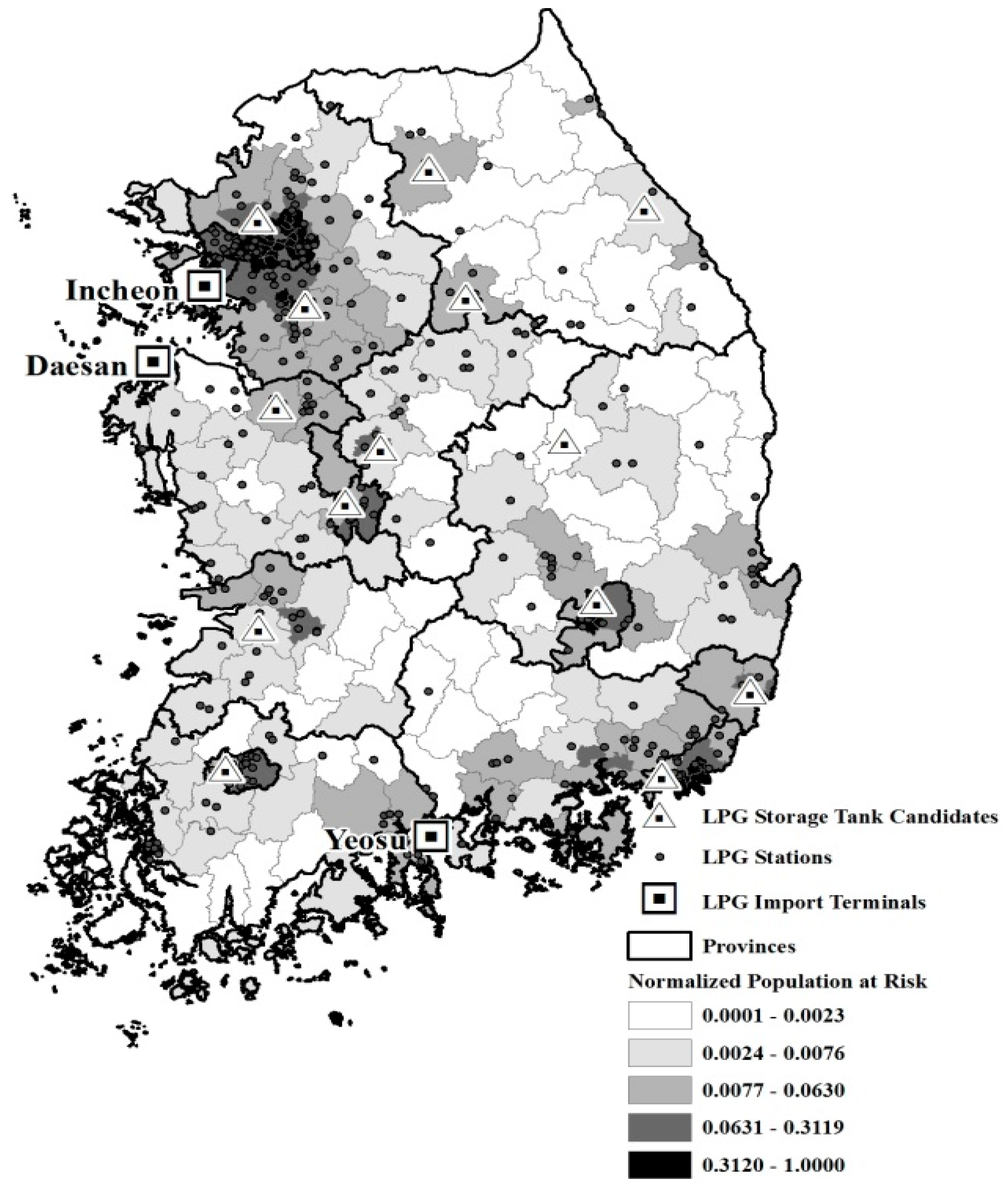
The remainder of this paper is organized as follows. Section 2 reviews relevant literature on the conceptual framework and measurement issues of resilience. Section 3 explains the DEA model and selected variables used in the model. Section 4 presents the application of the model to the SC of a case study of the LPG company in Korea and details the data collection and analysis results. Finally, Section 5 concludes the paper.

2. Literature Review

As the business environment is growing turbulent, designing SCNs has become a critical issue. To this end, SCR has received wide attention among both researchers and practitioners. Resilience has been defined by a number of disciplines and from various perspectives. From a general viewpoint, resilience is “the capacity for an enterprise to survive, adapt, and grow in the face of turbulent change” [25]. However, there is no unified definition for SCR, and researchers have coined their own definitions [11,12,16,25,26,27,28]. Among these, Maria Jesus Saenz et al. [11] unified the definition based on previous literature: the SCR is the capability of an enterprise to minimize the negative impacts of any unexpected error in its SC, by pursuing quick response to disruptive events and recovering to a desirable condition [11]. Such ability requires a more flexible SC, while accounting for the unstable nature of its activities [16]. An army of conceptual and theoretical papers studied the concept of resiliency in design of SCN, as the most important decision in strategic level that can facilitate the so-called readiness phase. In the following subsections, the conceptual foundation of the studies on SCR is reviewed first. Then, the quantitative studies that addressed supply chain resilience are surveyed.

2.1. Conceptual Foundation

Researchers have proposed conceptual frameworks to aid systematic understanding of resilience. Most studies considered vulnerability (catalyst of disruptions) and capability (ability to cope with disruptions) as major determinants of resilience. Some studies went further to analyze the relationship between vulnerability and capability. Chopra and Sodhi [29] identified sources of SC risks: disruptions, delays, systems, information processing, intellectual property, procurement, and receivables. To mitigate the risks, they claimed that firms can increase capacity (inventory), secure redundant suppliers, improve flexibility, and pool demand. Peck [30] posited that SC vulnerability occurs at four levels: value-stream/product or process (seamless flow of goods and information), assets and infrastructure dependencies (hardware and software capacity to handle product and information), organizations and inter-organizational networks (interplays among firms, public-private relationship), and environment (political, economic, social, and technological changes). They focused on vulnerability without considering capability. Christopher and Peck [12] categorized SC risk into internal, external, and environmental risks. Their framework suggests that bolstering resilience can be achieved through SC reengineering, SC collaboration, agility, and risk management culture. While the above studies treat vulnerability and capability factors somewhat separately, Pettit et al. [13] integrated vulnerability and capability factors into a single framework. They contend that vulnerability stems from forces of change, and capability can be developed through management control. They emphasize the balance between vulnerability and capability. Higher vulnerability compared with capability implies that firms are prone to SC disruptions, and higher capability means the loss of profitability.

By examining the terrorist attacks in 2001 from firms’ resilience perspective, Sheffi [6] viewed that resilience should be enhanced through insurance against emergency, redundant inventory policy, and knowledge/process backup. Moreover, he showed that trade-offs can occur between conventional business and resilient processes. For example, enterprises should decide between the lowest bidder or the known supplier, centralization or dispersion, redundancy or efficiency. Ponomarov and Holcomb [8] attempted to explain resiliency through control, coherence, and connectedness, originating from the field of psychology. They showed that conventional logistics strategies are included in the psychological domain of resilience. Jüttner and Maklan [31] empirically examined the role of SCR. They defined SCR capability as the combination of flexibility, velocity, visibility, and collaboration factors. They found that SC risk management and SCR capability significantly decreases SC vulnerability.

2.2. Measuring Resiliency of Supply Chain

Carpenter et al. [27] suggested that researchers should clearly answer two questions prior to measuring resiliency: (1) what type of system is to be resilient; and (2) what type of threats the system should be prepared for? Only after these two questions are made clear, one can proceed to developing or assessing a resilience measure. This paper analyzes resilience in the SC of LPG in response to the accidents (e.g., terrorist attacks and explosion) that halt its operation. In this regard, a number of influential factors are taken into consideration in the redesign of the SCN, to take preventive action within the “readiness” phase of building resilience and reduce the vulnerability of the SC. Keeping this in mind, this section summarizes the relevant studies that measured resiliency of SCNs based on individual factors. Existing studies used divergent resiliency measures, especially in the context of simulation or complex network theory. As is shown below, the researchers in this field do not have a unified view on the resilience index.

Priya Datta et al. [16] developed an agent-based simulation model to analyze the resilience of SCs, paying particular attention to the multi-product, multi-country case. They quantified resiliency using four measures: customer service level, production change over time, average inventory at each distribution center, and total average network inventory across all distribution centers. Spiegler et al. [32] used system dynamics to characterize SCs. They devised a measure called, “the integral of time multiplied by the absolute error” (ITAE). This measures how much the system strays from target customer service during the response and recovery periods of disruptions. Interestingly, they found that a robust SC—which retains performance even in disruption—is not necessarily resilient. Schmitt and Singh [17] examined a consumer packaged goods company, and order fill rate was selected as their performance measure. Their results showed that benefit of buffer stock increases exponentially when operation is disrupted. Using an agent-based simulation model, Wu et al. [33] analyzed retailers’ stockouts when products are heterogeneous. They used a downstream market share as a performance indicator. They found that customer types, initial market share, and stockout duration determine resiliency. Other studies used additional measures, which are listed in Table 1.

Another active area in resilience studies utilizes topological measures to characterize resilient systems. They are grounded on complex network theory. Xu et al. [21] considered topological characteristics of the network to assess resilience, using such indicators as the degree of distribution, average path length, and clustering coefficient. Mari et al. [20] classified ideal topological characteristics of a resilient network, based on four different influential factors: accessibility, robustness, flexibility, and responsiveness. They found that the size of the largest functional network, the clustering coefficient, and the characteristic path length in the largest functional part are critical for improving the robustness, flexibility, and responsiveness of the SC, respectively. Similar conclusions were drawn by Hearnshaw and Wilson [19], who claimed that resilience can be enhanced by high levels of connectivity, a short characteristic path length, and a high clustering coefficient. The latter two measures, however, are mostly dependent on the type of product and service, and the competitive advantage of the system. Hence, industry characteristics should be reviewed carefully for the results to be meaningful. Huang et al. [34] analyzed the network of emergency logistics. They examined two measures, namely the effective demand node ratio and supply mileage, to evaluate the reliability of a network. Peng et al. [15] developed an “anti-attack model” to describe recovery behavior from external threats. Node degree was only used in measuring resilience performance. In a critical review on the resiliency of SCN, Perera et al. [35] suggested incorporating operational indicators, such as flows, costs, and capacities, as well as conventional topological measures.

Other studies have used measures based on survey scales. Some of these even proposed a resilience index. Zsidisin and Wagner [18] estimated the relationships among flexibility, redundancy, and risk sources on disruption occurrences. They posited that resiliency represents the reciprocal of disruption occurrences, such as late delivery, quality problem, excess costs, and the use of alternate sources. They found that flexibility and redundancy moderates the effect of supply market risk on disruption occurrences. Töyli et al. [36] postulated that robustness (preparedness) and agility are indicators for resiliency. Not surprisingly, they found that higher resiliency, attained by bolstering agility and robustness, enhances an SC’s customer value. Pettit et al. [14] proposed an SCR framework and developed a resilience index measure, based on capability and vulnerability. In addition, a resilience balance measure was created due to firms experiencing reduced profits, otherwise damaged from disruptions when one of the qualities was insufficient. Azadeh et al. [23], and Azadeh and Salehi [22], evaluated the resilience of petrochemical plants using DEA. They defined management commitment, reporting culture, learning, awareness, preparedness and flexibility, self-organization, teamwork, redundancy, and fault-tolerance as desirable outputs. The rationale of their approach is that increasing these factors is preferred for resilience.

Reviewing relevant papers, the following gaps are found in the SCN literature. First, only a few studies sought to assess resilience through developing an index. Even the few extant studies developed the resilience index based on survey scales, which can hinder the performance evaluation of a specific system in relation to others. Survey-based resilience indexes (like the one developed by Azadeh et al. [23], and Azadeh and Salehi [22]) can also lead to biased measurements as survey respondents report their opinions subjectively. It is believed, therefore, that the analysis in the present study is more robust than the survey-based approach because it evaluates resilience based on quantitative data, such as available capacity, node degree, clustering coefficient, and total distance in supply chains. Through the DEA, the data is aggregated to yield a single resilience index for individual SCN. In other words, the resilience index (or score) is used as a standard for assessment. Moreover, none of the existing studies attempted to provide a resolution for enhancing resiliency based on the developed resilience index. This last issue is addressed in the present study through the introduction of slack measures that is interpreted as the extent to which the existing configuration should be altered to improve resiliency in the SC.

3. Methodology

3.1. DEA Model

This study employs DEA to evaluate SCR. Developed by Charnes et al. [24], DEA is a programming-based technique that has been widely used to assess the performance of decision-making units (DMUs), i.e., any subjects to be evaluated such as organizations or teams. Its focus is to identify best-practice frontier in an industry and measures the distance between the frontier and individual business unit performance. In other words, DEA is a peer-evaluation technique, where best-practice and less-performing DMUs are identified among observed DMUs. DMUs are more credible with less input redundancy and output shortfalls compared with other firms. Prior to applying the DEA, one should assume that the followings hold:

(1)

There is no measurement error in the data.

(2)

If DMUs (network configurations) are observed to operate with certain input and output sets, the combination of the input and outputs sets are also operable (convexity).

(3)

If a specific network configuration can operate with a certain input and output set, it can also operate at a point that uses larger input and yields less output (strong disposability).

Numerous DEA models have been developed since Charnes et al.’s seminal work. Most of them adopted radial measures of performance. For example, the resulting performance score requires equiproportional change of input reduction or output expansion. A prime reason for preferring radial measure lies in its mathematical tractability. Researchers can easily manipulate or identify properties of models when radial measures are used. This, however, was challenged by some researchers because equiproportional input reduction or output expansion may not be realistic [43,44,45,46]. Instead, DMUs in practice would seek to identify the greatest source of inefficiency among inputs or outputs, and prioritize its improvement.

To address this shortcoming using radial measures, this paper uses a slacks-based performance measure (SBM) as proposed by Tone [47]. This approach is a non-radial and non-orientation model, therefore capturing the more realistic nature of the business world and providing more practical solutions. The model is specified as follows:

$$\mathrm{Minimize}\theta =\left(1-\frac{1}{M}{\displaystyle \sum _{i=1}^M\frac{s_i^{-}}{x_{io}}}\right)/\left(1+\frac{1}{N}{\displaystyle \sum _{r=1}^N\frac{s_r^{+}}{y_{ro}}}\right)$$

(1)

which is subject to

$${\displaystyle \sum _{k=1}^K{\lambda }_k{x}_{ik}=}{x}_{io}-s_i^{-},i=1,...,M$$

(2)

$${\displaystyle \sum _{k=1}^K{\lambda }_k{y}_{rk}}=y_{ro}+s_r^{+},r=1,...,N$$

(3)

$${\lambda }_k,s_i^{-},s_r^{+}\ge 0,\forall k,i,r.$$

(4)

where $\theta \in [0,1]$ is the performance index, $x_{ik}$ is the observed input of DMU k for input type i, and y_rk is the observed output for output type r. $s_i^{-}$ and $s_r^{+}$ are slacks, which represent reducible or expandable input and output amounts, respectively. M and N denote the number of inputs and outputs, respectively. The objective function (1) finds the full extent of input or output improvement potential. In constraint (2), the left-hand side is the best-practice input level for a DMU. This equation further expresses that the best-practice level can be attained by reducing current input levels $x_{io}$ by $s_i^{-}$. Likewise, in Equation (3), the best-practice level of output ${\displaystyle \sum _{k=1}^K{\lambda }_k{y}_{rk}}$ can be reached once output increases the currently operating level $y_{ro}$ by $s_r^{+}$. Considered together, the SBM model identifies maximum improvement potentials at individual input and output levels (hence, a non-radial model), and more importantly, DMUs are directed to reduce inputs and increase outputs simultaneously (hence, non-orientation model).

When measuring resiliency, however, having more inputs should be considered as advantageous, as keeping redundant capital or labor can contribute to a swift recovery from disruption. To account for this, variables are redefined as positive, negative, and external factors. Positive and negative factors are those that have a direct impact on the resilience of a system and firms can control. Those other than positive and negative factors were classified as the external factor, which exert an indirect impact on resilience while firms have limited control over them. As introduced in Section 1, positive factors increase resilience while negative factors decrease resilience when their respective values are increased. External factors marginally affect resilience but should be managed closely to minimize potential impacts. This means that SCN alternatives that are characterized with higher external factors should carefully consider resilience. Hence, $x_{io}$ is labeled as negative or external factors, and $y_{ro}$ positive factors, where the former and the latter provide better results at reduced values and at increased values, respectively.

3.2. Selected Variables

3.2.1. Positive Factor

Available Capacity

One of key tenets of resiliency is securing redundant inventory or capacity [9,14,29]. Hence, the available capacity is included to measure resiliency. It is calculated by using the following formula:

$$AvailableCapacity=TotalCapacity\times AvailabilityRate.$$

(5)

Total capacity is the total supply capacity over all nodes in the SCN. It should be noted that some capacity cannot be used when faced with disruptions. In other words, when some nodes are disrupted, existent capacity cannot be utilized. To reflect this possibility, the availability rate is included in the formula, which is the proportion of available capacity to total capacity in the time of disturbance. The availability rate was obtained through what-if analysis.

In conducting what-if analysis, hypothetical scenarios for random or targeted attacks were made, and their effects on LPG flows were analyzed. A random attack refers to a circumstance in which all the nodes in the network can be under attack with equal likelihood. Conversely, targeted attack means that attackers target the most significant nodes in terms of roles or characteristics. While examining both scenarios can be meaningful, this paper focuses on the targeted attack due to one crucial reason: the number of demand nodes is substantially higher than the number of supply nodes. Thus, if attacks are purely random, the attack would most likely involve demand nodes due to its larger number, although potential assailants would more likely target the most vulnerable and impactful supply nodes.

The process for assessing targeted attacks was performed as follows: The supply nodes with the most connections were chosen from listing supply nodes by their number of connections and their capacity for each configuration (DMU). Using the model detailed in the Appendix A, total capacity was determined. The supply node with the most connections was assumed shut down by attacks, one at a time. The outcome of this step was used in Equation (5) as the availability rate.

Node Degree and Clustering Coefficient

According to Hearnshaw and Wilson [19], topological (or geographical) measures, including power law connectivity distribution and clustering coefficients, are key determinants of an efficient SCN. Other researchers have advocated the use of these measures in evaluating SCs [21,48,49]. Both indicators represent how SC nodes are interconnected. Greater connectivity implies higher resiliency [50] because those high-connecting suppliers have more alternatives to supply goods, increasing the possibility of avoiding disruptions in nodes. Thus, these indicators were used as positive factors, comprised of an average node degree and an average clustering coefficient.

The average node degree (AND) is the average number of connections per node, calculated by

$$AND=\frac{1}{N}{\displaystyle \sum _{i=1}^N{k}_i},$$

(6)

where N is the network size, i.e., the total number of neighbors of all nodes, and K_i the number of connection of node i. Complementarily, the average clustering coefficient (ACC) measures the degree of mutual exchange connections among the nodes in the network by using the following formula:

$$ACC=\frac{1}{N}{\displaystyle \sum _{i=1}^N\frac{N_i}{k_i(k_i-1)/2}},$$

(7)

where N_i is the number of neighbors of node i. In the case study that follows, K_i was calculated through ArcGIS. It is noteworthy that both AND and ACC measures can be calculated based on a connection matrix, which results from the hub-location allocation model described in the Appendix A.

Number of Supply Nodes

The next operational measure, the number of supply nodes, is one of the major factors in designing SCNs. If this indicator is low, the SC is more likely to be centralized. As detailed in previous literature [9,29], employing fewer nodes lengthens recovery when a node is disrupted. In addition, when an explosion happens within a centralized SC, e.g., LPG, the impact on the adjacent population would be more severe because the scale of the explosion would increase with the degree of facility centralization. In other words, the more supply nodes employed in the SCN, the smaller the capacity of each individual supplier compared with a centralized system; therefore, the magnitude of explosion in the presence of such inflammable material will be less. To account for these aspects, the number of supply nodes is used as a positive factor. This factor is referred to as p in the Appendix A, by which the number of nodes chosen for the optimal configuration of the SCN is considered.

3.2.2. Negative Factor

Only total distance was used as a negative factor. This denotes the total distance between supply and demand nodes. Chen and Lin [48] suggest that less total distance results in increased resiliency as decentralization generally reduces the total distance in the outbound logistics, as well as the whole system. Moreover, higher total distance means that an SC faces higher demand, and if disrupted, the effects on supply would be much worse.

3.2.3. External Factor

In addition to positive and negative factors, an external factor, population density, was incorporated into the model. It is posited that the external factor may not affect an SCR directly. It can, however, exert considerable damage on the society if a supply facility from that SC is under risk. For example, owing to the inflammability of LPG, the potential damage to the people around a storage tank in case of a possible explosion can be substantial, if the population at risk is high. Moreover, the business can suffer from significant restructuring if people recognize the potential danger involved in that SC. Hence, if an SCN puts more population at risk, the firm should watch the SCR more closely.

4. Application of the Model to a Case Study in Korea

In the present study, the proposed DEA-based approach is applied to the case of a LPG company in Korea. The choice of the firm seems appropriate due to the strategic role of fuel in the daily life and its hazardous nature as a inflammable liquid. For this purpose, different SC configuration scenarios are compared and assessed in terms of resiliency (see

Table 2. LPG supply chain data.

SCN Config.	Ave. Node Degree	Clustering Coefficient (105)	No. of Supply Nodes	Available Capacity (Ton)	Total Distance (Km)	Population Density *
1	1.995	0.000	2	53,002.5	162,700	4452
2	2.000	0.015	3	77,996	160,200	4652
3	2.000	0.008	3	56,401.172	131,010	9308
4	2.011	0.104	4	80,070.852	127,770	4940
5	2.000	0.008	3	57,487.392	131,010	9308
6	2.011	0.104	4	80,781.569	127,770	4940
7	2.011	0.133	4	57,815.846	106,600	6411
8	2.022	1.600	5	85,005.144	106,870	13,895
9	2.011	0.133	4	59,357.692	106,600	6411
10	2.022	1.600	5	87,422.65	106,870	13,895
11	2.028	0.628	5	59,890.152	101,270	13,554
12	2.049	4.130	6	85,179.567	96,459	13,650
13	2.028	0.628	5	62,120.714	101,270	13,554
14	2.049	4.130	6	87,644.823	96,459	13,650
15	2.049	1.360	6	60,072.998	89,489	14,191
16	2.077	9.640	7	85,752.84	74,066	9084
17	2.049	1.360	6	62,357.684	89,489	14,191
18	2.077	9.640	7	88,436.857	74,066	9084
19	2.077	3.830	7	61,021.554	67,730	17,880
20	2.109	28.200	8	86,936.811	72,123	13,373
21	2.077	1.360	7	63,626.922	67,730	17,880
22	2.109	9.640	8	90,025.922	72,123	13,373

* This value is obtained by summating the number of people over the SCN that are located within a radius of 480 m in the neighborhood of supply node.

for details).

4.1. Case Study: LPG Supply Chain in Korea

The SCN of “E1”, a major Korean company in the fuel sector, has been chosen for analysis. E1 accounts for approximately half of the LPG import demand in Korea. E1 imports LPG from oil-producing countries using three terminals in Korea, Incheon, Yeosu, and Daesan (see Figure 1). LPG is stored in Incheon and Yeosu terminals with capacities of 76,000 and 69,000 tons, respectively. Such a centralized supply network has various advantages and disadvantages. 75% of the capacity is reserved for transportation fuels, and the rest is used for industrial, petrochemical, and residential purposes. Daesan terminal does not service gasoline for automobiles, but has the capability to do so when operation in the other two terminals is compromised. This paper considers only transportation fuels because this accounts for the majority of the company’s operations. In the current network configuration, there is no intermediate storage tank (IST). Considering risk factors to the people around the three-mentioned terminals, any kind of explosion can be catastrophic due to the huge amount of stored LPG in few supply nodes. Moreover, any operational disruption in Incheon or Yeosu terminals can noticeably interrupt LPG supply in Korea. To this end, E1 considers opening ISTs to increase resilience. Data collection procedure is detailed in the following section.

4.2. Data Collection

Figure 2 shows the process for data analysis used in the case study. Once primary data for SCN configurations and population density were collected, the values for the other variables used in the DEA models were calculated using ArcGIS 10.2, and MATLAB R2015b. More detailed processes for data collection can be summarized as follows.

First, the data on the E1’s SC facilities and population was collected and then refined and mapped using ArcGIS. Second, 14 candidates for the ISTs were chosen by running the relevant module in ArcGIS and considering a set of criteria, including accessibility to road networks for all the station nodes, while avoiding high population density areas. Third, the hub-location allocation problem coded in MATLAB software was employed to find the optimum solution for total distance in the system for each of the pre-defined number of supply nodes. The required capacity for each configuration was also estimated using the total assigned demand for each IST. More specifically, the location allocation optimization module in the ArcGIS software was employed to assign stations to supply nodes. Then, the total distance of a full truck-load shipping system was calculated using ArcGIS. Fourth, the connection matrix of each individual solution resulting from the optimization process was extracted using MATLAB software, enabling for calculation of the average node degree and clustering coefficient. For details of the connection matrix produced by the hub-location allocation optimization problem, see Appendix A. Fifth, available capacity for disruption was estimated using the what-if analysis, as previously discussed. Finally, the population exposure data was estimated using ArcGIS software to approximate the number of people affected by the disruption in each supply node, within a radius of 480 m, following Kim and Bae [51].

Table 2 and

Table 3. Summary statistics of variables.

Variable	Min	Med.	Max.	Std.
Positive Factor
Available capacity (Tons)	53,002.5	70,811.5	90,025.9	13,239.2
Ave. node degree	2.0	2.0	2.1	0.0
Clustering coefficient (105)	0.0	1.4	28.2	6.2
Number of supply nodes	2.0	5.0	8.0	1.7
Negative Factor
Total distance (Km)	67,730.0	101,270.0	162,700.0	27,147.0
External Factor
Population density	4452.0	13,373.0	17,880.0	4166.7

report the prepared data set and descriptive statistics. The first column in Table 2 characterizes the profile of different SCN configurations. Since the number and overall capacity of supply nodes in each echelon of SC are among the main features to describe its network, these are selected to configure each DMU in Table 2. Accordingly, two possible options are considered for the number and overall capacity of supply nodes in the first echelon. For example, the network configurations with the same number of supply nodes are either designed to have a capacity equal to the overall demand, or to be able to hold a buffer in addition to the required capacity. The number of intermediate facilities in the second echelon is considered as the next factor, where the decided level for this factor is determined considering the sample adequacy check. To be more specific, the SC No. 1 represents the current SC configuration, where only two import terminals are active to supply LPG to the automobile gas stations. The SC No. 2 indicates the same single echelon distribution network but with three active import terminals. The rest of the configurations consider a two-echelon SCN with one to five intermediate facilities, respectively.

Previous literature suggests that the total number of DMUs should be three times higher than the total number of input and outputs, for the results to be considered reliable [52]. Therefore, five possible levels for the number of intermediate facilities is decided in order to satisfy the mentioned requirement.

Note that the positive factor of clustering coefficient contains zero observations. Because DEA is based on linear programming, zero data in the denominator variable (y) in Equation (1) is not workable. To address this issue, the recommendation by Tone [47] was employed as follows:

$$y_o\leftarrow \frac{1}{10}\min \left\{y_j|y_j>0,j=1,...,n\right\}$$

(8)

That is, the zero observations are substituted by a tenth of the minimum positive value among observations. This way, an SCN with zero positive factors can become eligible for the DEA. The inflation of the values would not affect results significantly because its extent is so small.

5. Results and Discussion

Table 4. Resilience scores in SCN alternatives of E1.

SCN Config.	Resiliency Score	Ranking	Resiliency Score Considering Population Density	Ranking Considering Population Density
1	0.000	22	1.000	1
2	0.001	19	1.000	2
3	0.001	20	0.002	21
4	0.008	17	0.998	9
5	0.001	21	0.002	22
6	0.008	18	1.000	3
7	0.012	15	0.128	17
8	0.127	11	0.154	13
9	0.012	16	0.128	18
10	0.127	12	0.154	14
11	0.058	13	0.069	19
12	0.293	7	0.338	11
13	0.058	14	0.069	20
14	0.260	8	0.300	12
15	0.131	10	0.142	16
16	0.639	6	0.992	10
17	0.132	9	0.143	15
18	0.642	5	1.000	4
19	1.000	1	1.000	5
20	1.000	2	1.000	6
21	1.000	3	1.000	7
22	1.000	4	1.000	8

presents the resiliency scores, where the scores are given in the form of decimal numbers between zero and one. The “zero” score indicates the worst-performing network configuration relative to others (in terms of resilience), while the best-practices are given a score of 1. The second and fourth columns report the resulting score before and after factoring population density into the analysis, respectively. Looking at the plain resilience score, the discriminatory power is rather high, i.e., only four SCN configurations 19–22, are resilient. This indicates that the DEA results in the present study are dependable [52]. This can also be interpreted as a signal to stop inclusion of new configurations to the analysis, which requires addition of more supply nodes and capacity to the SCN. Note that resilient scores vary widely across different configurations. SCN configurations, such as 1–7, receive very low resilience scores, meaning that they are most vulnerable to disruptions. Considering the fourth column, however, some of the SCN configurations considered to be vulnerable become resilient when population risk is taken into account. For example, the resilience scores in SCN numbers 1, 2, 6, 18 increase dramatically when population risk is considered. This is due to the relatively lower population density in the mentioned configurations, resulting in negligible impacts on the people around the supply nodes when serious accidents occur. In other words, the SCR is sufficient and features little need for improvement with respect to population concerns.

Table 5. Resilience slacks in SCN alternatives of E1 without considering the population factor.

SCN Config.	Available Capacity (Ton)	Average Node Degree	Clustering Coefficient	Number of Supply Nodes	Total Distance (Km)
1	143,115.5	3	63.6	16	0
2	115,108.5	3	62.6	15	0
3	101,517.8	2	51.2	12	0
4	73,942.7	2	49.9	10	0
5	100,431.6	2	51.2	12	0
6	73,231.9	2	49.9	10	0
7	70,679.4	1	41.5	8	0
8	43,815.6	1	40.2	7	0
9	69,137.6	1	41.5	8	0
10	41,398.1	1	40.2	7	0
11	62,180.4	1	39.0	6	0
12	31,091.8	1	33.6	5	0
13	59,949.8	1	39.0	6	0
14	28,626.5	1	33.6	8	0
15	47,796.7	1	33.6	4	0
16	3526.1	0	19.3	1	0
17	45,512.0	1	33.6	4	0
18	842.0	0	19.3	1	0
19	0.0	0	0.0	0	0
20	0.0	0	0.0	0	0
21	0.0	0	0.0	0	0
22	0.0	0	0.0	0	0

lists slacks in the DEA model not including the population factor. They indicate that the degree of each resilience factor (positive and negative) of the SCN at the current norm (Configuration No. 1) should improve to enhance SCR to a certain point. For instance, SCN 1 should increase its available capacity by 143,116 and its average node degree by 3 to achieve the highest resilience. This way, it is observed that network configurations of the alternative SCs lacking in resilience tend to require additional efforts for increasing resilience, even if they offer a better level of resiliency comparing to the current norms. However, the total distance is an exception to this claim. In other words, it can be concluded that total distance (negative factor) is not a significant determinant of resiliency based on these results.

Table 6. Resilience slacks in SCN alternatives of E1 with population factor.

SCN Config.	Available Capacity (Ton)	Average Node Degree	Clustering Coefficient	Number of Supply Nodes	Total Distance (Km)	Population Density
1	0.0	0	0.0	0	0.0	0
2	0.0	0	0.0	0	0.0	0
3	25,128.8	0	15.2	3	37,133.0	0
4	710.7	0	0.0	0	0.0	0
5	24,042.6	0	15.2	3	37,133.0	0
6	0.0	0	0.0	0	0.0	0
7	24,783.5	0	3.5	1	0.0	0
8	5325.1	0	27.7	3	31,931.8	0
9	23,241.6	0	3.5	1	0.0	0
10	2907.6	0	27.7	3	31,931.8	0
11	28,223.3	0	28.0	3	28,170.8	0
12	3558.0	0	24.7	2	22,842.1	0
13	25,992.8	0	28.0	3	28,170.8	0
14	1092.7	0	24.7	5	22,842.1	0
15	32,181.6	0	28.6	2	12,954.4	0
16	2684.0	0	0.0	0	0.0	0
17	29,896.9	0	28.6	2	12,954.4	0
18	0.0	0	0.0	0	0.0	0
19	0.0	0	0.0	0	0.0	0
20	0.0	0	0.0	0	0.0	0
21	0.0	0	0.0	0	0.0	0
22	0.0	0	0.0	0	0.0	0

displays the slack results after incorporating population density into the analysis. Interestingly, the pattern of slacks in Table 6 is different from those in Table 5. Current average node degree is sufficient, but total distance requires additional reduction. This may be because more residents are exposed to the danger of accidents when supply routes are longer (longer total distance). Moreover, increasing node degree may expose more people to supply chain disruption. However, though this study did not intend to restrict population density value, model results are more realistic in that population density has zero slacks. Otherwise, having positive slack values for this variable can be considered unrealistic, since the population density cannot be changed to solve the resilience problem in practice.

The SCN rankings of both models with and without the population factor and the slack measures provide SC managers with useful decision-making guidelines for examining to what extent resiliency of the current network should be improved. On the other hand, it should be noted that some of the systems lacking in resilience under the first model (no population factor model), such as SC 1, 2, 5 and 18, resulted in being resilient when the population factor was considered. This is in contrast with the results of previous studies [21,48,49], which claim that an increase in each of the positive factors of clustering coefficient and average node degree (as individual factor), or considering additional capacity [9,14,29] leads to redundancy, and in turn improves resiliency of the SCN. The results of the present study, however, show that this is not always true as shown in Table 6, especially when more comprehensive factors such as population exposure risk are considered. Therefore, this indicates that the estimation of resiliency as a relative measure among possible SCN configurations should be conducted with simultaneous consideration of divergent and conflicting factors, as used in this study.

6. Conclusions

This research assesses the SCR using the DEA. Acknowledging resiliency as a strategy for the design of SCN [53], the present study attempted to score alternative SCN configurations with respect to different factors. To this end, a number of topological and operational characteristics that affects the resilience of the LPG supply chain are further considered. The developed approach proposes a unique framework of applying DEA to evaluate resiliency. Traditional DEA approaches assume that input redundancy and output shortfalls are “bad”. In contrast, redundancy in this study is a primary requirement for resilient SCs, so SCNs with more inputs, e.g., redundant capacity, should receive more credit from a resiliency viewpoint. From this perspective, variables were classified into three types. First, positive factors are a set of variables that enhance resilience if their values are increased. Available capacity, average node degree, clustering coefficient, and the number of supply nodes were included as positive factors. Conversely, negative factors are variables that deteriorate resiliency when their values increase. In the analysis provided in this research paper, total distance traveled was included in this category. Lastly, external factors represent the variables that do not directly affect resiliency, but can exert significant negative effects, in tandem with other factors, when an SC is disrupted. Population density was used as an external factor.

The resilience model was applied to a case study of an LPG handling company in Korea, E1. The results show that the SCN of the analyzed firm, E1, needs substantial improvement. The low resilience configuration featured small values for all positive factors. When population density was included in the model, the average node degree required no improvement, whereas reduction in total distance was necessary. This implies that average node degree is not necessarily important to mitigate population risk, but reduction in total distance is a critical factor.

The approach used in this study can be used for both academia and industry, as resiliency in an SCN can be measured in relation to the alternative configurations. Moreover, comprehensive factors influencing resiliency are simultaneously considered in the developed approach in the present research. The proposed approach provides a useful decision-making framework for examining investment decisions for the resiliency of SC. The provided ranking and slack measures provide insight for trade-offs between the required investment to change SC system, and consequential benefits by the enhanced SCR. This is the first study to consider population exposure risk together with other relevant factors in SCR.

This paper also provides managerial implications. Three strategies are recommended to enhance the resiliency of the SCN configuration. First, SCR planners should consider both direct shipping to gas stations, as well as shipping to gas stations through intermediate storage tanks. In doing so, alternative supply nodes would be available when a specific node breaks down. Second, interconnection among the supply nodes is suggested for facilitating exchange among suppliers when necessary. Finally, to cope with capacity shortfalls in periods of disruption, managers should consider retaining excess capacity. However, if this option is limited, due to a lack of budget for example, they can discriminate between different demand nodes according to demand elasticity or the other relevant criteria. For example, the demand nodes which are located in the strategic regions should be served as top priority.

Future research can extend results of the present study in several ways. In comparing SCN configurations of LPG, the analysis is confined to a single company. Future studies can broaden data used in analysis by evaluating SCNs covering multiple firms. This analysis identifies the profile of less resilient and resilient firms, which is effective in drawing managerial implications, such as how vulnerable firms can increase their resilience. Moreover, inclusion of more operational measures such as delivery time and total cost incurred for a specific SCN, would improve index reliability. When the proposed method is applied to service logistics and online shopping cases, shortages, and backorder costs can be incorporated to strengthen the analysis. Lastly, this paper assumes that higher capacity is always better to increase resilience, as numerous authors have assumed implicitly, e.g., Pettit et al. [14], Azadeh and Salehi [22], and Azadeh et al. [23]. However, excessive capacity has negative aspects from the managerial viewpoint, as this increases costs associated with maintenance and storage. Therefore, a more desirable approach would determine minimum excess capacity that can ensure swift recovery and reduce costs simultaneously. When additional data on actual damage and recovery are collected, one can assess the extent to which the capacity of DMUs should be enhanced to improve resilience considering the trade-off between increased cost and benefit of reduced damage, and the recovery cost.

References

1. Pourhejazy, P.; Kwon, O.K. The New Generation of Operations Research Methods in Supply Chain Optimization: A Review. Sustainability 2016, 8, 1033. [Google Scholar] [CrossRef]
2. Christopher, M.; Towill, D. An Integrated Model for the Design of Agile Supply Chains. Int. J. Phys. Distrib. Logist. Manag. 2001, 31, 235–246. [Google Scholar] [CrossRef] [Green Version]
3. Mason-Jones, R.; Naylor, B.; Towill, D.R. Lean, Agile or Leagile? Matching Your Supply Chain to the Marketplace. Int. J. Prod. Res. 2000, 38, 4061–4070. [Google Scholar] [CrossRef]
4. Lamming, R. Squaring Lean Supply with Supply Chain Management. Int. J. Phys. Distrib. Logist. Manag. 1996, 16, 183–196. [Google Scholar] [CrossRef]
5. Naylor, J.B.; Naim, M.M.; Berry, D. Leagility: Integrating the Lean and Agile Manufacturing Paradigms in the Total Supply Chain. Int. J. Prod. Econ. 1999, 62, 107–118. [Google Scholar] [CrossRef]
6. Sheffi, Y. Supply Chain Management under the Threat of International Terrorism. Int. J. Logist. Manag. 2001, 12, 1–11. [Google Scholar] [CrossRef]
7. Lee, H.L. The Triple—A Supply Chain. Harv. Bus. Rev. 2004, 82, 102–113. [Google Scholar] [PubMed]
8. Ponomarov, S.Y.; Holcomb, M.C. Understanding the Concept of Supply Chain Resilience. Int. J. Logist. Manag. 2009, 20, 124–143. [Google Scholar] [CrossRef]
9. Sheffi, Y.; Rice, J.B., Jr. A Supply Chain View of the Resilient Enterprise. MIT Sloan Manag. Rev. 2005, 47, 41. [Google Scholar]
10. Sheffi, Y. The Resilient Enterprise: Overcoming Vulnerability for Competitive Advantage; MIT Press Books: Cambridge, MA, USA, 2005; Volume 1. [Google Scholar]
11. Hohenstein, N.; Feisel, E.; Hartmann, E.; Giunipero, L. Research on the Phenomenon of Supply Chain Resilience: A Systematic Review and Paths for further Investigation. Int. J. Phys. Distrib. Logist. Manag. 2015, 45, 90–117. [Google Scholar] [CrossRef]
12. Christopher, M.; Peck, H. Building the Resilient Supply Chain. Int. J. Logist. Manag. 2004, 15, 1–14. [Google Scholar] [CrossRef] [Green Version]
13. Pettit, T.J.; Fiksel, J.; Croxton, K.L. Ensuring Supply Chain Resilience: Development of a Conceptual Framework. J. Bus. Logist. 2010, 31, 1–21. [Google Scholar] [CrossRef]
14. Pettit, T.J.; Croxton, K.L.; Fiksel, J. Ensuring Supply Chain Resilience: Development and Implementation of an Assessment Tool. J. Bus. Logist. 2013, 34, 46–76. [Google Scholar] [CrossRef]
15. Peng, H.; Lu, S.; Zhao, D.; Zhang, A.; Li, J. An Anti-Attack Model Based on Complex Network Theory in P2P Networks. Phys. A Stat. Mech. Its Appl. 2012, 391, 2788–2793. [Google Scholar] [CrossRef]
16. Priya Datta, P.; Christopher, M.; Allen, P. Agent-Based Modelling of Complex Production/Distribution Systems to Improve Resilience. Int. J. Logist. Res. Appl. 2007, 10, 187–203. [Google Scholar] [CrossRef]
17. Schmitt, A.J.; Singh, M. A Quantitative Analysis of Disruption Risk in a Multi-Echelon Supply Chain. Int. J. Prod. Econ. 2012, 139, 22–32. [Google Scholar] [CrossRef]
18. Zsidisin, G.A.; Wagner, S.M. Do Perceptions Become Reality? The Moderating Role of Supply Chain Resiliency on Disruption Occurrence. J. Bus. Logist. 2010, 31, 1–20. [Google Scholar] [CrossRef]
19. Hearnshaw, E.J.; Wilson, M.M. A Complex Network Approach to Supply Chain Network Theory. Int. J. Phys. Distrib. Logist. Manag. 2013, 33, 442–469. [Google Scholar] [CrossRef]
20. Mari, S.I.; Lee, Y.H.; Memon, M.S.; Park, Y.S.; Kim, M. Adaptivity of Complex Network Topologies for Designing Resilient Supply Chain Networks. Int. J. Ind. Eng. 2015, 22, 102–116. [Google Scholar]
21. Xu, N.; Liu, J.; Li, D.; Wang, J. Research on Evolutionary Mechanism of Agile Supply Chain Network via Complex Network Theory. Math. Probl. Eng. 2016, 2016, 1–9. [Google Scholar] [CrossRef]
22. Azadeh, A.; Salehi, V. Modeling and Optimizing Efficiency Gap between Managers and Operators in Integrated Resilient Systems: The Case of a Petrochemical Plant. Process Saf. Environ. Prot. 2014, 92, 766–778. [Google Scholar] [CrossRef]
23. Azadeh, A.; Salehi, V.; Ashjari, B.; Saberi, M. Performance Evaluation of Integrated Resilience Engineering Factors by Data Envelopment Analysis: The Case of a Petrochemical Plant. Process Saf. Environ. Prot. 2014, 92, 231–241. [Google Scholar] [CrossRef]
24. Charnes, A.; Cooper, W.W.; Rhodes, E. Measuring the Efficiency of Decision Making Units. Eur. J. Oper. Res. 1978, 2, 429–444. [Google Scholar] [CrossRef]
25. Fiksel, J. Sustainability and Resilience: Toward a Systems Approach. Sustain. Sci. Pract. Policy 2006, 2, 14–21. [Google Scholar] [CrossRef]
26. Pereira, J.V. The New Supply Chain's Frontier: Information Management. Int. J. Inf. Manag. 2009, 29, 372–379. [Google Scholar] [CrossRef]
27. Carpenter, S.; Walker, B.; Anderies, J.M.; Abel, N. From Metaphor to Measurement: Resilience of What to What? Ecosystems 2001, 4, 765–781. [Google Scholar] [CrossRef]
28. Sheffi, Y. Preparing for the Big One [Supply Chain Management]. Manuf. Eng. 2005, 84, 12–15. [Google Scholar] [CrossRef]
29. Chopra, S.; Sodhi, M.S. Managing Risk to Avoid Supply-Chain Breakdown. MIT Sloan Manag. Rev. 2004, 46, 53. [Google Scholar]
30. Peck, H. Drivers of Supply Chain Vulnerability: An Integrated Framework. Int. J. Phys. Distrib. Logist. Manag. 2005, 35, 210–232. [Google Scholar] [CrossRef]
31. Jüttner, U.; Maklan, S. Supply Chain Resilience in the Global Financial Crisis: An Empirical Study. Supply Chain Manag. Int. J. 2011, 16, 246–259. [Google Scholar] [CrossRef]
32. Spiegler, V.L.; Naim, M.M.; Wikner, J. A Control Engineering Approach to the Assessment of Supply Chain Resilience. Int. J. Prod. Res. 2012, 50, 6162–6187. [Google Scholar] [CrossRef]
33. Wu, T.; Huang, S.; Blackhurst, J.; Zhang, X.; Wang, S. Supply Chain Risk Management: An Agent-Based Simulation to Study the Impact of Retail Stockouts. IEEE Trans. Eng. Manag. 2013, 60, 676–686. [Google Scholar] [CrossRef]
34. Huang, L.; Wang, W.; Wang, M. Simulation Research of Space-Time Evolution of Emergency Logistics Network Reliability Based on Complex Network Theory. Discret. Dyn. Nat. Soc. 2013, 2013, 1–7. [Google Scholar] [CrossRef]
35. Perera, S.S.; Bell, M.; Bliemer, M. Modelling Supply Chains as Complex Networks for Investigating Resilience: An Improved Methodological Framework. In Proceedings of the 37th Australasian Transport Research Forum (ATRF), Sydney, Australia, 30 September–2 October 2015.
36. Wieland, A.; Marcus Wallenburg, C. The Influence of Relational Competencies on Supply Chain Resilience: A Relational View. Int. J. Phys. Distrib. Logist. Manag. 2013, 43, 300–320. [Google Scholar] [CrossRef]
37. Barroso, A.P.; Machado, V.H.; Machado, V.C. The Resilience Paradigm in the Supply Chain Management: A Case Study. In Proceedings of the 2011 IEEE International Conference on Industrial Engineering and Engineering Management (IEEM), Singapore, 6–9 December 2011; pp. 928–932.
38. Carvalho, H.; Barroso, A.P.; Machado, V.H.; Azevedo, S.G.; Machado, V.C. Supply Chain Resilience: A Simulation Study. Ann. DAAAM Proc. 2011, 2011, 1611–1613. [Google Scholar]
39. Carvalho, H.; Barroso, A.P.; Machado, V.H.; Azevedo, S.; Cruz-Machado, V. Supply Chain Redesign for Resilience using Simulation. Comput. Ind. Eng. 2012, 62, 329–341. [Google Scholar] [CrossRef]
40. Ishfaq, R. Resilience through Flexibility in Transportation Operations. Int. J. Logist. Res. Appl. 2012, 15, 215–229. [Google Scholar] [CrossRef]
41. Kristianto, Y.; Gunasekaran, A.; Helo, P.; Hao, Y. A Model of Resilient Supply Chain Network Design: A Two-Stage Programming with Fuzzy Shortest Path. Expert Syst. Appl. 2014, 41, 39–49. [Google Scholar] [CrossRef]
42. Wang, J.; Gao, F.; Ip, W.H. Measurement of Resilience and its Application to Enterprise Information Systems. Enterp. Inf. Syst. 2010, 4, 215–223. [Google Scholar] [CrossRef]
43. Chang, Y.; Park, H.; Jeong, J.; Lee, J. Evaluating Economic and Environmental Efficiency of Global Airlines: A SBM-DEA Approach. Transp. Res. D 2014, 27, 46–50. [Google Scholar] [CrossRef]
44. Charnes, A.; Cooper, W.W.; Golany, B.; Seiford, L.; Stutz, J. Foundations of Data Envelopment Analysis for Pareto-Koopmans Efficient Empirical Production Functions. J. Econ. 1985, 30, 91–107. [Google Scholar] [CrossRef]
45. Cook, W.D.; Seiford, L.M. Data Envelopment Analysis (DEA)—Thirty Years on. Eur. J. Oper. Res. 2009, 192, 1–17. [Google Scholar] [CrossRef]
46. Portela, M.; Thanassoulis, E. Developing a Decomposable Measure of Profit Efficiency using DEA. J. Oper. Res. Soc. 2007, 58, 481–490. [Google Scholar] [CrossRef]
47. Tone, K. A Slacks-Based Measure of Efficiency in Data Envelopment Analysis. Eur. J. Oper. Res. 2001, 130, 498–509. [Google Scholar] [CrossRef]
48. Chen, H.; Lin, A. Complex Network Characteristics and Invulnerability Simulating Analysis of Supply Chain. J. Netw. 2012, 7, 591–597. [Google Scholar] [CrossRef]
49. Zhao, K.; Kumar, A.; Harrison, T.P.; Yen, J. Analyzing the Resilience of Complex Supply Network Topologies against Random and Targeted Disruptions. IEEE Syst. J. 2011, 5, 28–39. [Google Scholar] [CrossRef]
50. Callaway, D.S.; Newman, M.E.; Strogatz, S.H.; Watts, D.J. Network Robustness and Fragility: Percolation on Random Graphs. Phys. Rev. Lett. 2000, 85, 5468. [Google Scholar] [CrossRef] [PubMed]
51. Kim, K.H.; Bae, J.W. A Dispatching Method for Automated Guided Vehicles to Minimize Delays of Containership Operations. Int. J. Manag. Sci. 1999, 5, 1–25. [Google Scholar]
52. Cooper, W.W.; Seiford, L.M.; Zhu, J. Data envelopment analysis. In Handbook on Data Envelopment Analysis; Springer: New York, NY, USA, 2004; pp. 1–39. [Google Scholar]
53. Carvalho, H. Modeling Resilience in Supply Chain (Thesis). Faculdade de Ciências e Tecnologia. Available online: http://hdl.handle.net/10362/8949 (accessed on 10 February 2017). (In English)
54. Hakimi, S.L. Optimum Distribution of Switching Centers in a Communication Network and some Related Graph Theoretic Problems. Oper. Res. 1965, 13, 462–475. [Google Scholar] [CrossRef]
55. Hakimi, S.L. Optimum Locations of Switching Centers and the Absolute Centers and Medians of a Graph. Oper. Res. 1964, 12, 450–459. [Google Scholar] [CrossRef]
Figure 1. LPG supply chain network in Korea based on population at risk.
Sustainability 09 00255 g001
Figure 2. Data collection procedure.
Sustainability 09 00255 g002