Analysis of Landscape Patterns of Arid Valleys in China, Based on Grain Size Effect


1
Linze Inland River Basin Research Station, Chinese Ecosystem Research Network, Key Laboratory of Eco-hydrology of Inland River Basin, Northwest Institute of Eco-Environment and Resources, Chinese Academy of Sciences, Lanzhou 730000, China
2
University of Chinese Academy of Sciences, Beijing 100049, China
3
College of Earth Sciences and Resources, Chang’an University, Xi’an 710054, China
*
Author to whom correspondence should be addressed.
Sustainability 2017, 9(12), 2263; https://doi.org/10.3390/su9122263
Submission received: 2 November 2017
/
Revised: 2 December 2017
/
Accepted: 5 December 2017
/
Published: 13 December 2017
(This article belongs to the Special Issue Advances and Applications in Measuring, Representing, and Comparing Spatial Landscape Patterns)
Abstract
:Landscape metrics are useful tools in investigating spatial structure and in describing the heterogeneity of landscapes, but are sensitive to grain size. Thus, it is necessary to determine the appropriate grain size before researching landscape patterns. However, there have been few large-scale investigations in high-precision research about the effect of grain size on landscape patterns, especially in arid valleys in China. Thus, we selected three representative sample areas according to the basic characteristics of arid valleys, and we chose 22 grain sizes from 15 to 450 m to calculate twelve landscape metrics at the landscape level and six landscape metrics at the class level to analyze the most appropriate grain size for the arid valleys. All basins in the study area were converted to an appropriate-sized grid to analyze the landscape patterns. Our results showed that the effect of grain size on landscape metrics can be categorized as: no law, increasing, decreasing, or no change. The majority of the fitted landscape index curves were good, with high R2 values. The most appropriate grain size at both levels was 75 m. The landscape pattern of arid valleys was scale-dependent. At the landscape level, arid valley landscape patterns changed from northwest to southeast due to topography and hydrothermal conditions. While the value of aggregation for different size classes was high, the other metrics showed significant differences due to area and degree of human activity at the class level.
1. Introduction
Landscape metrics are widely used to investigate spatial structure and describe the heterogeneity of landscapes [1,2,3,4,5]. It is important to consider the effects of scale on interpretation of spatial heterogeneity and its ecological consequences [6]. With improved calculations and methods for analyzing landscape patterns, assessing the scale effect on landscape pattern metrics has been a key area of research in landscape ecology [7].
Scaling functions are the most precise and concise way of explicitly quantifying multiscale characteristics [8,9,10]. In landscape research, the scale effect is generally considered in spatial and temporal contexts [6,11]. Spatial scale is a central variable in research on landscape patterns and has two important components: extent and grain size [12,13]. Extent is the total length, area, or volume that exists or is analyzed; grain size is the basic landscape unit, affecting not only the precision and accuracy of the calculation but also the validity and completeness of the information extracted [14,15]. The choice of grain size depends on the study objectives and the landscape characteristics. When grain size is closest to the actual scale of the landscape in question, interpretations of landscape patterns are most accurate [16].
Our understanding of landscape spatial heterogeneity, including landscape patterns, functions, and processes, is dependent on the scale and resolution used for observations [17]. With the accumulation of historical data and the development of remote sensing, including geographic information systems (GIS) and other technologies, making examination of the “scale effect” more feasible and significant but complicating the issue of how to determine the scale to use in macroscopic research [18]. The advancement of landscape technical methods, especially application of the software FRAGSTATS [19], facilitates the large-scale study of scale effects on landscape heterogeneity.
The scale effect depends on many factors [20]. Examination of the ways in which pattern metrics change with scale in real landscapes will improve understanding of scale-dependent spatial heterogeneity [17]. Disturbances lead to variations in natural scale [21]. The response of landscape metrics to changing grain size is influenced by zonality and spatial heterogeneity, which vary significantly across landscapes [22]. The effect of landscape metrics on the choice of grain size has been examined by many ecologists. The metrics value is sensitive to land-cover composition and to misclassification of land cover [23]. Spatial patterns have a strong influence on interpretation of species diversity [24]; insects and vertebrate diversity is widely used in conservation management and is scale-dependent [5,25]. Scale-dependent landscape metrics can also be used to analyze highly linked hydrological processes [26]. Moving-window analyses of spatial patterns in floodplains at multiple scales showed that scale influences all surface metric values and their spatial organization [27].
The use of landscape metrics has become popular in efforts to quantify and characterize landscape patterns with remote data and technology [1,2,3]. Although most landscape metrics are sensitive to changes in spatial extent, spatial resolution, and thematic resolution, the sensitivity varies among metrics and study areas [1,3]. The optimum scale and landscape pattern analysis need to be combined to increase the accuracy in landscape measurements [3]. Metrics have three types of responses to grain size: predictable responses with simple scaling relations, staircase-like responses without simple scaling relations, and erratic responses without general scaling relations [17]. Scale-related studies have focused on various topographic areas in China, including plains [28], hills [29,30], mountains [31,32], and habitats such as settled landscapes and ecotones [33]. With rapid urbanization, researchers have examined the effects of grain size on understanding of landscapes such as urban and urban–rural transitional areas [34]. Some researchers have performed comparative analyses of different patches within a given area, or of similarities and differences in the effects of grain size on landscape classification, to explore the relationships between patch type and size and grain size [35]. Under the optimum scale identified by multiresolution analysis, landscape patterns can be measured well [9,10].
Arid valleys are ecologically important features of mountainous landscapes in China, and finding the grain size of arid valley landscapes is important to helping ensure regional ecological security and to promote environmental protection measures appropriate to local conditions [36]. In recent years, there has been severe aridification and secondary aridification (human activity-induced aridification) of arid valleys. At the same time, the geothermal energy usage of these valleys has enabled concentrated population growth, despite their limited land area, which has led to degradation of biological diversity and regional ecological functioning [37,38]. There is an urgent need to address the ways in which scale affects interpretation of arid valley landscape patterns under human influence. Areal extent and grain size should be determined prior to describing landscape patterns. Thus, this paper has four objectives: (1) to determine how extent influences landscape patterns in arid valleys by using three different-sized sample areas; (2) to determine how landscape metrics change with grain size and how grain size influences our understanding of landscape patterns; (3) to determine whether extent or grain size has a more significant effect on interpretation of arid valley landscapes; and (4) to determine the most appropriate grain size for analyzing landscape characteristics of arid valleys at the landscape and class levels.
2. Materials and Methods
2.1. Study Area
The Hengduan Mountains are located in the southeastern region of the Qinghai-Tibet Plateau, adjacent to the northwestern boundary of Yunnan Province. They range from 24°40′N to 34°00′N lat and from 96°20′E to 104°30′E long [39]. This area is part of China’s subtropical climate zone, under the influence of high-elevation westerly wind currents, the Indian Ocean, and the Pacific monsoon. Winters are dry, and summers are very rainy. There is a distinct division between the dry and wet seasons; wet season normally occurs from May to October, with precipitation accounting for 75 to 90% of the annual total [40]. Dry season occurs from October to April; precipitation during this period is under 30 mm in most of the meteorological stations in the Hengduan Mountains [41]. Arid valleys are unique natural landscapes of the Hengduan Mountains region in southwestern China. These valleys mainly occur along the Jinsha, Nujiang, Lancangjiang, Yuanjiang, Yalong, Minjiang, Dadu, and Anning rivers and some of their tributaries [36]. Arid valleys are relatively fragile ecosystems that are susceptible to natural disasters such as debris flows, collapse, and landslides due to having steep slopes. These valleys have deep rivers and north–south mountain ranges that minimize the influence of the southeastern Pacific monsoon and the southwestern Indian Ocean monsoon. Coupled with the “foehn effect” (strong, warm dry winds), the valleys are dry and hot, sparsely vegetated, and have low levels of land cover. The climate of the arid valleys has a clear vertical distribution. The Hengduan Mountains are well-known for their biodiversity [42], but they have low plant diversity and cover, and more shrubs than trees. Shrubs are the dominant drought-tolerant species; their morphological adaptations to dry conditions include thorns and hairiness. The soils are acidic and include red soils and heavy clay. Most arid valley soils are leached, iron- or aluminum-enriched, thin, and severely eroded and degraded as a result of human activity [37].
Research on arid valleys in the Hengduan Mountains advanced in the 1980s and focused primarily on physical features, such as soil and soil-forming characteristics, vegetation, species richness [43], temperature and hydrology. Arid valleys have been classified into four subcategories based on temperature and hydrology: dry-hot, dry-warm, dry-lukewarm, and dry-cool; these categories are used to determine the most appropriate plant species for different areas [36].
There has been little research on Hengduan Mountain arid valleys in the 21st century, although some studies have examined environmental degradation, development issues, and protection measures in relation to climate change. Data from 27 meteorological stations in the Hengduan Mountains from 1961 to 2012 reflect a decrease in precipitation extremes from southwest to northeast [44]. More specifically, the average temperature of arid valleys in the Hengduan Mountain area increased by 0.11 °C per decade, but relative humidity and sunshine hours showed a decreasing trend [45]. The ability of ecosystems in the region to adapt to these changes was investigated [46], and research on sustainable development has been pursued [47]. A summary of basic research indicates that the extent of arid valleys has increased and that habitat quality has deteriorated, and research on ecological restoration has been recommended [38]. Other work in arid valleys in the Hengduan Mountains has focused on specific features such as rivers. Most river research was performed in the upper reaches of the Minjiang River [48], and the Jinsha [49], Lancangjiang [50], and Dadu [51] rivers. Other research has focused on administrative areas, mostly in Sichuan Province [51,52]. These studies show that the boundaries of arid valleys have been expanding while environmental conditions have been worsening.
2.2. Methods
2.2.1. Sample Selection
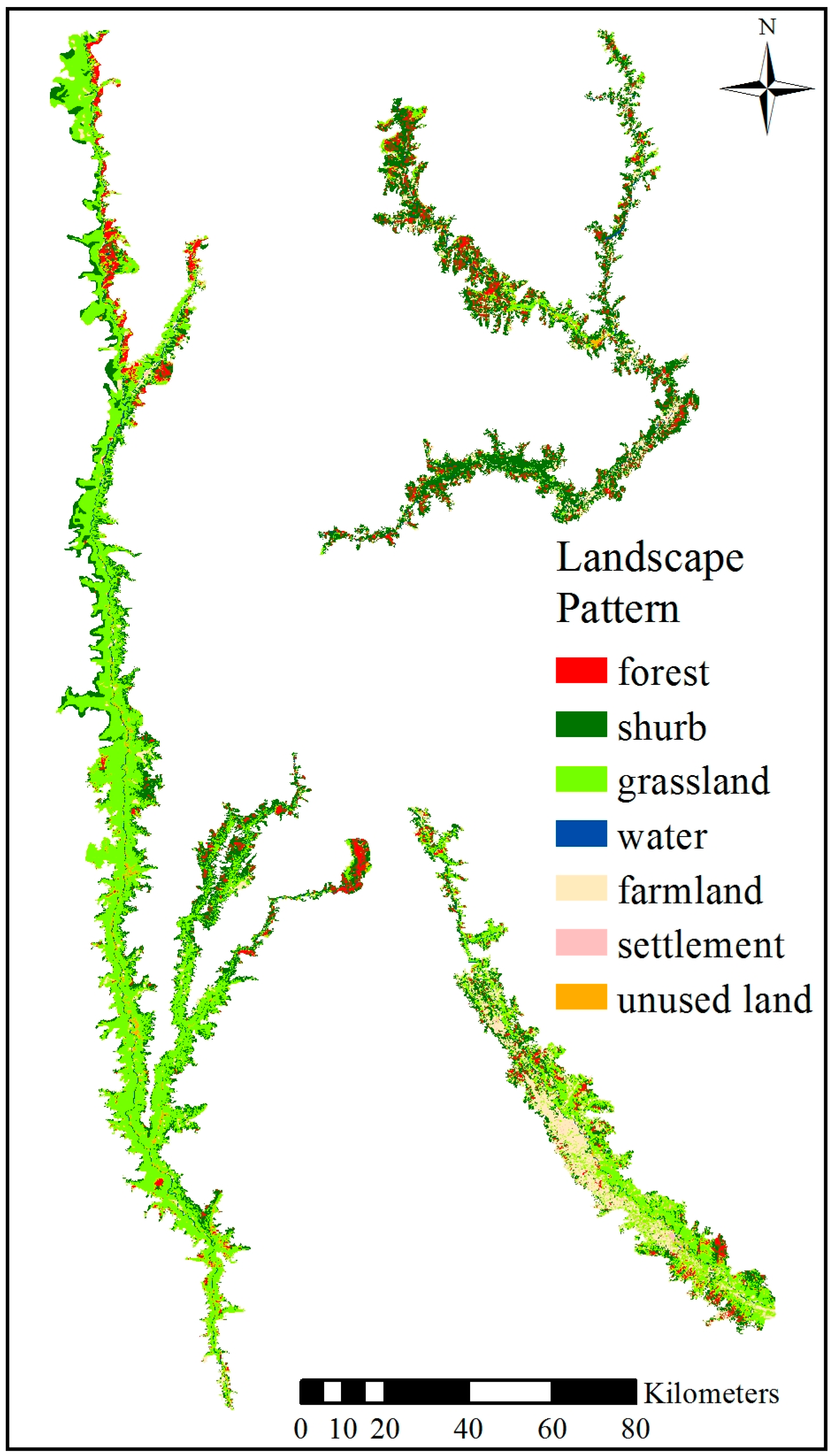
Based on the range of arid valleys, we selected 32 good-quality images within the study area from 2014 LANDSAT 8 data [53]. Using remote sensing software such as ArcGIS and ENVI, the boundaries of the arid valleys were obtained and the spatial distribution of the valleys was determined. In ENVI 5.1, these data were changed by Tasseled Cap Transformation, and the ISODATA Unsupervised Classification tool was used to divide the study area into seven categories: forest, shrub, grassland, water, farmland, settlement, and unused land. The overall accuracy was 85.7%, indicating that the classification result was accurate.
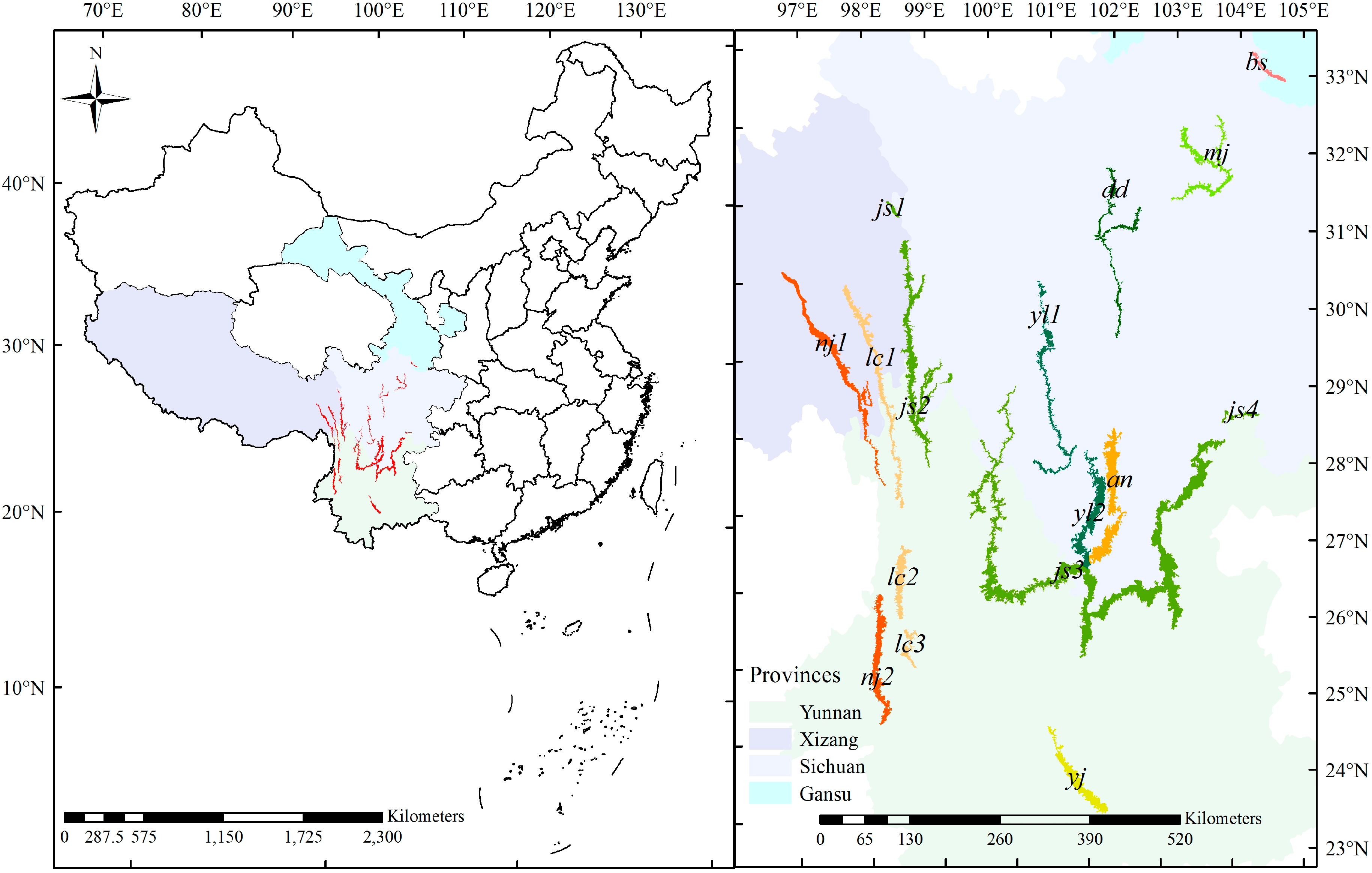
To ensure that calculated landscape pattern metrics were meaningful, discontinuous arid valleys were marked from north to south and from west to east. For example, the Jinsha River has four discontinuous valleys, which were labeled js1, js2, js3, and js4. We used the same method to mark the Nujiang, Lancang, and Yalong river valleys (Figure 1).
We first calculated basal data for the valleys in the eight river basins (Table 1). To reduce the amount of data and to obtain more intuitive observations of basin characteristics, three samples were selected: arid valleys in the upper reaches of the Jinsha River, characterized by large areal extent, high elevation, steep slopes, a grassland landscape matrix, and minimal impact from human activity; the arid valley in Minjiang River, which has relatively small areal extent, low elevation, gentle slopes, a shrub landscape matrix, and moderate human influence; and the arid valley in Yuanjiang River, with small areal extent, low elevation, gentle slopes, a grassland matrix, and severe anthropogenic influence (Figure 2).
2.2.2. Choice of Landscape Metrics and Grain Size
Landscape metrics include the patch, class, and landscape levels. We considered six types of landscape metrics: area and edge, shape, core area, contrast, aggregation, and diversity. We chose 12 metrics at the landscape level (Table 2) and six metrics at the class level: percentage of landscape (PLAND), number of patches (NP), PD, LPI, PAFRAC, and AI (The same as the landscape level metrics in Table 2).
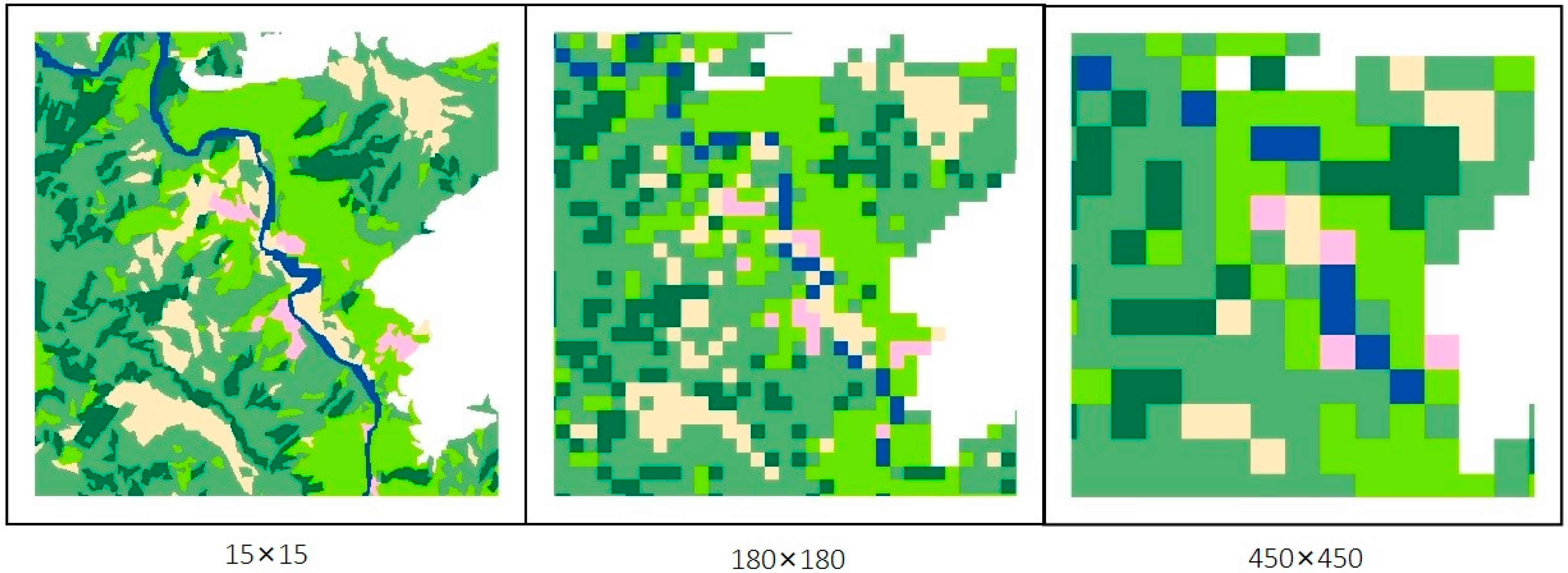
Landscape pattern data were transformed into GRID raster data for FRAGSTATS 4.2 [54] in ESRI’s ArcGIS 10.0 [55]. We selected 22 landscape grain sizes from 15 m to 450 m. We used a grain-size interval of 15 m between 15 m and 210 m, and an interval of 30 m between 210 m and 450 m. Figure 3 shows images of the same site using grain sizes of 15 m, 180 m, and 450 m. As the patch resolution is reduced, landscape boundaries become smoother and detail is lost.
The calculated data were imported into Origin 8.5 [56] to complete a map of the impact of landscape metrics on grain size effect. Using the curve-fitting function and regression analysis in SPSS 19.0, the functional relationship between landscape metrics and grain size was established, and the strength of the correlation was tested.
3. Results
3.1. Impact of Landscape Metrics
3.1.1. Landscape Level
Grain Size Response Curve
We used FRAGSTATS to calculate 12 landscape-level metrics for the three samples using 22 grain sizes, and a response curve for landscape size and performance index in relation to grain size was generated. The values for total area (TA) varied greatly so the grain size effect of this index for the three samples were shown separately; the other 11 metrics were placed on one map of the three sample areas for comparison (Figure 4).
There were four types of response curves for the 12 metrics:
Type I: No-law scaling relations. Area and edge, specifically TA and LPI, are Type-1 metrics. With changing grain size, these metrics show small-amplitude fluctuations with no obvious regularity or characteristic function. Fluctuations in TA increase and become less regular with increasing grain size, so accuracy was greater at smaller calculation scales. For LPI, the patch index at 30 m, 90 m and 210 m identified the inflection point, but there was no obvious change in the law.
Type II: Increasing scaling relations. This response curve corresponds to PAFRAC in the shape metric and IJI in the aggregation metric. The PAFRAC response curve has inflections at 30 m and 210 m, and the whole curve is smoother. The IJI response curve has inflection points at 60 m and 180 m; the index of arid valley js2 begins to be disordered at 195 m, while the response curves of mj and yj fluctuate greatly after 300 m.
Type III: Decreasing scaling relations. This response curve corresponds to FRAC_MN in the shape metric. Its curve is concave and tends to stabilize after the inflection point at 150 m. In addition, aggregation metrics with the exception of IJI have this relationship. The curves of NP and PD are convex, flat, and mostly stable after the inflection point at 300 m. The SPLIT curve declines rapidly before 45 m and then gradually begins to flatten. The AI curve is concave and flattens after 330 m. The response curve of LSI decreases linearly with slight waves at 45 m, 150 m, and 220 m.
Type IV: No change in scaling relations. This response curve corresponds to diversity metrics, including SHDI and SHEI. The curve is stable and unaffected by grain size, with only a small change in amplitude after 195 m.
Curve Fitting
Simulation by SPSS 19.0 (Table 3).
The greatest effect of grain size on landscape metrics in the three samples can be well simulated by the different functions. There is no suitable function to simulate the effects of TA, SHDI, or SHEI, and simulation of LPI and SPLIT is poor. The shape metric can be simulated well, with precision > 95%; PAFRAC fits a logarithmic function, average shape index, and FRAC_MN is a cubic function. LSI and AI are simulated using cubic functions; IJI is also cubic, but only js2 has precision > 90%. Of the aggregative metrics, NP and PD can be simulated with exponential functions, with fitting precision > 98%.
The first scale domain and the appropriate grain size were obtained from the response curves and simulation results for the 12 landscape level metrics (Table 4). The first scale domain at the landscape level is 60–90 m, and the optimum size is 75 m. For a single index, the scale domain is divided based on the inflection point of the index curve [57]. In the first scale domain, selecting the appropriate grain size can not only reflect the characteristic information of the landscape better, but also avoid the redundant computation [58]. The overlap of the appropriate grain size for each index is the optimum size for landscape pattern research for each index can be best explained in this grain size.
3.1.2. Class Level
Grain-Size Response Curve
In FRAGSTATS, 22 grain sizes for six landscape metrics at the class level were calculated for the three samples, and response curves were generated for landscape size and performance index according to grain size (Figure 5).
There were four types of response curves for the six metrics:
Type I: No law for scaling relations. This response curve applies to LPI. The values for water decrease sharply at 45 m and values for grassland increase at 45 m for js2. The js2 index is more stable from 60 to 120 m; mj is stable from 45 to 180 m, and yj is stable from 60 to 195 m.
Type II: Increasing scaling relations. This response curve also applies to LPI, showing an increasing trend but fluctuating after 135 m. Changes in the water class differ from other patches, showing a decreasing tendency in js2, but increasing before decreasing in mj and yj. The farmland and settlement classes fluctuate more strongly than other landscape patches.
Type III: Decreasing scaling relations. This response curve includes NP, PD, and AI. The curves of NP and PD are convex, and the response curve for water has a parabolic trend. All classes in AI show a concave, declining trend. The grain-size response curve of js2 and mj fluctuate after 150 m, and the curve of yj fluctuates after 120 m.
Type IV: No change in scaling relations. This response curve applies mostly to PLAND. The curve of js2 does not change with increasing grain size, but the mj and yj curves fluctuate after 125 m and 135 m, respectively. Thus, smaller index sizes are better.
Curve Fitting
Curve fitting simulated by SPSS 19.0 (Table 5).
The PLAND and LPI curve simulations are not good. All classes in the NP response curve can be simulated by cubic functions, with precision > 95% except for water. Curve fitting is the same for PD and NP. In PAFRAC, forest, shrub, grassland, farmland, and unused land take power functions with precision > 95%, but water and settlement are fitted with cubic functions with low precision. The classes in AI are well simulated, with precision > 94%; all classes take exponential functions, except grassland and farmland in js2 and mj, which are described by cubic functions.
According to the response curves and the simulation results for the six class-level landscape metrics, the first scale domain and the appropriate grain size were obtained (Table 6). The first scale domain at the class level is 60–135 m, and the optimum size is 75 m.
3.2. Landscape Pattern
In conclusion, the most suitable size for arid valleys is 75 m at both the landscape and class levels. The spatial data were transformed into grid data with 75 m grain size in ArcGIS 10.0, and the landscape metrics were then calculated in FRAGSTATS 4.2.
3.2.1. Landscape Level
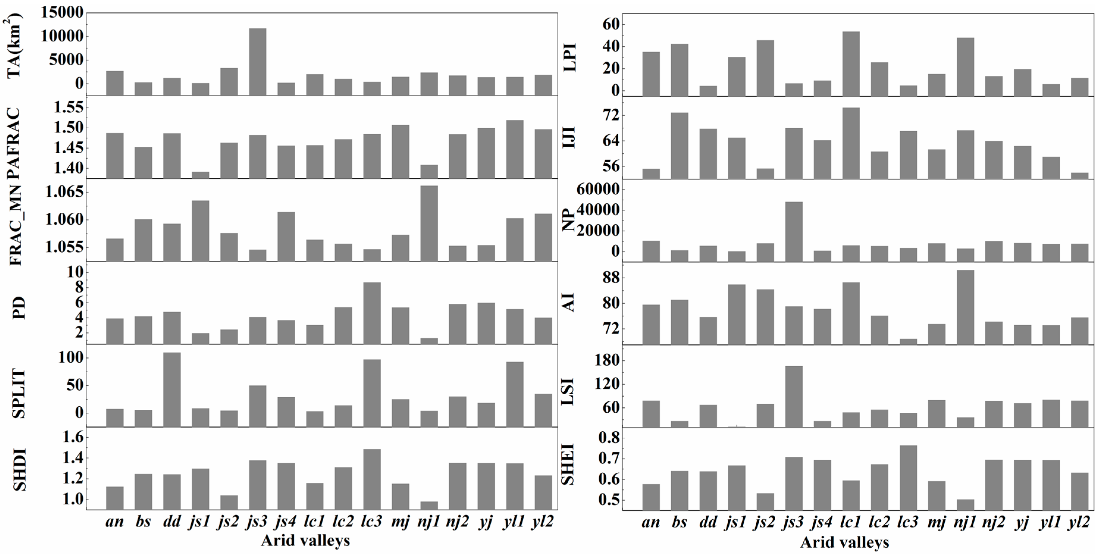
The six landscape metrics calculated at the landscape level are shown in Figure 6.
TA has the following characteristics: the area of js3 exceeds 10,000 km2 and is significantly larger than the other basins. The landscape area of js1, js4, yj, and lc3 is <500 km2. The area of the other basins is between 1000 and 3500 km2. NP shows the same trend as TA. The PD of lc3 is largest and has the greatest uniformity; the PDs of js1 and js2 are low with more uniform landscape, and the others are intermediate.
From the calculation results for LPI, there is a dominant patch in nj1, js2, js4, lc3, and bs. The first four valleys have high elevation, steep terrain, little human disturbance, and thus little fragmentation. However, the area of basin bs is small, so it has consistent patches that dominate. Basin an has low elevation and flat terrain; an has been developed into a wide, uniform area of cultivated land, so the LPI value is just 35. Basins lc3 and js1 are small and have intermediate LPI. The other LPI values are <20, have no dominant patches, and are more fragile.
The calculated PAFRAC values of the arid valleys are between 1.4 and 1.5, which indicate that landscape shape has intermediate complexity, with climatic and human influences, and follows a rule. The calculation results for SPLIT show that valleys lc3, yl1, and dd have a greater degree of broken landscape, and smaller basins such as an, have a unified landscape.
FRAC_MN shows a moderate level of shape complexity of patches. In comparison, the shape of nj1 and js1 are more complex. However, nj2, lc, an, and yj have the most simple landscape shape.
IJI can reflect the distribution characteristics of ecosystems that are restricted by natural conditions. The calculated values of js2, yl2, and an are low, which indicates that these ecosystems are severely affected by vertical zonality and human activity, so their patches are distributed, and aggregation is low. AI expresses the degree of connectivity of the patches. It can be seen that the least amount of shared boundary between patches occurs in lc3, and connectivity between patches is greatest in nj1, js1, and js2. LSI shows the degree of aggregation of like patches, which is greatest in js3.
SHDI and SHEI are widely used in community ecology to indicate landscape diversity and uniformity. The results reflect landscape heterogeneity and are especially sensitive to the uneven distribution of patch types. The trends of these two indicators are basically the same. Basin lc3 has the highest value, indicating that the landscape has high fragmentation and large uncertainty. The values of nj1, lc1, and js2 are relatively low, indicating strong landscape integrity, a low degree of fragmentation, and a small amount of information. The other valleys are intermediate between these two scenarios.
3.2.2. Class Level
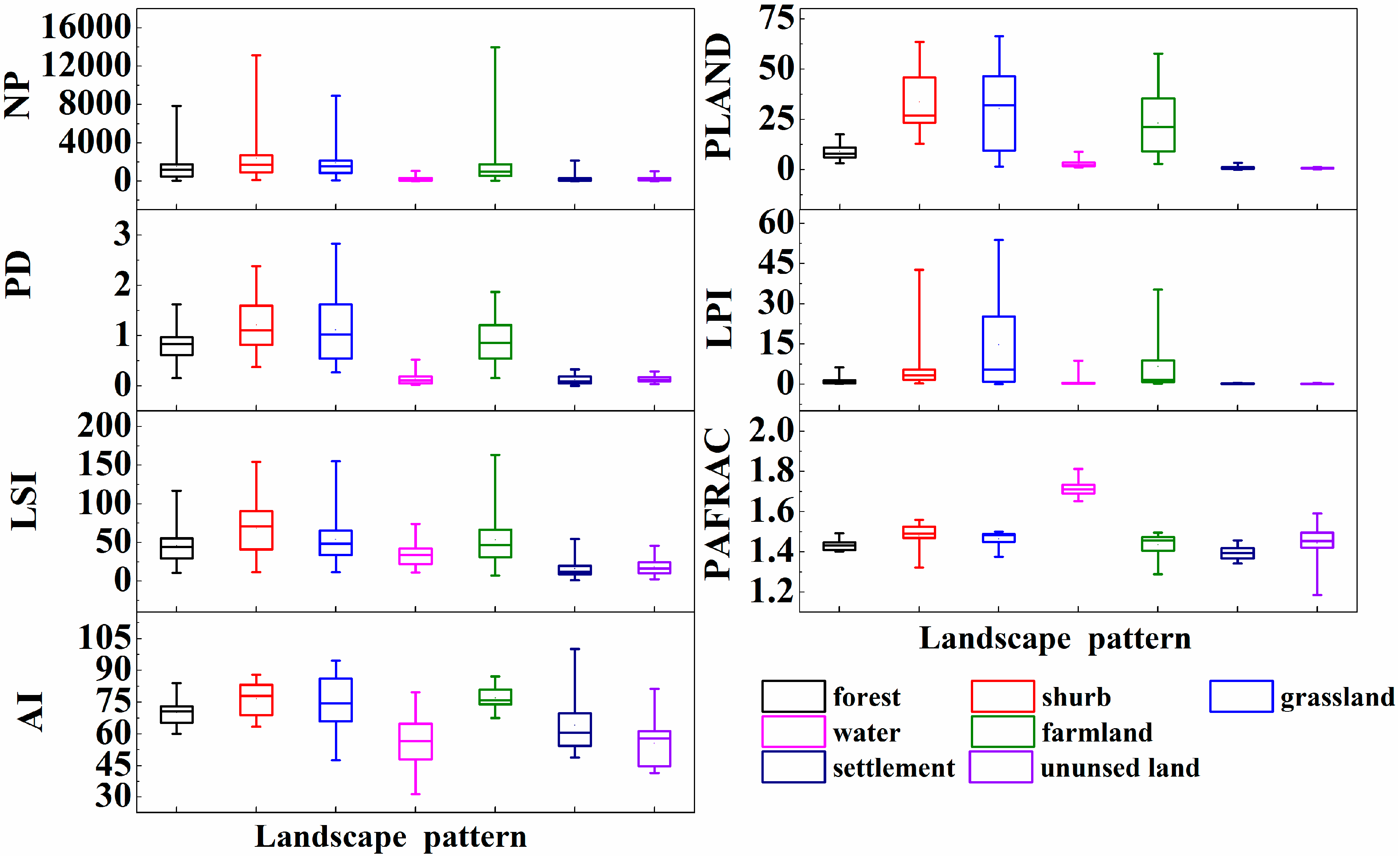
Landscape metrics of arid valleys at the class level were calculated for the different basins (Figure 7).
PLAND represents how much of the total landscape area a given patch type accounts for. The proportion of water, settlement, and unused land in all basins occupies less than 10%, and the proportion of forest is also generally small, less than 20% of the total area. The landscape matrix in bs, dd, mj, and yl2 is shrub, and the matrix in js, lc, nj, and yj is grass. The proportion of forest and grassland patches is almost equal in yj1. Major anthropogenic influence is apparent in basins an, js4, lc3, and nj2, which have a large proportion of farmland (>50% of the total area in an).
NP represents the number of patches in the landscape. NP is high in js3 because of its large area. The same tendencies are seen in other basins: the NPs of water, settlement, and unused land are low; farmland is the next lowest; the NPs of forest and grassland are equal; and shrub has the greatest number of patches. NP and PLAND are related, but the correlation is not entirely positive. For example, in the arid valley of an, although farmland occupies the largest proportion of landscape area, farmland patches are large and regular, so there are fewer patches of farmland compared to forest and shrub.
PD represents the number of patches per unit area. Landscape classes with low NP (water, settlement, unused land) also have low PD. The shrub class has the largest number of patches in an, js, and yl1, where it also has the largest PD. In bs, dd, nj, yj, mj, grassland has the highest PD, indicating that grassland is the most widely distributed landscape class. PD is not inevitably related to the landscape matrix. Although the landscape matrix always has the largest area of all landscape classes, PD is also affected by the degree of fragmentation and anthropogenic activity.
LPI represents the proportion of the largest patch of a given type in the whole landscape. The dominant patch types are shrub in bs, mj, and yl2; grassland in js1, js2, lc1, nj, and yj; and farmland in an and lc2. The other basins have no obvious dominant patch. LPI is positively correlated with PLAND.
PAFRAC represents the shape distribution of patches. The river corridor has the most irregular shape and the highest PAFRAC value. Patches that represent severe human influence, i.e., settlement and farmland, are uniform and have low PAFRAC values. The calculated values of the shrub class in js1 and nj1 are relatively low, which may be related to the use of shrub-type economic crops in arid valleys.
AI indicates the degree of polymerization of the same patch type. Water is generally distributed in the center of the arid valleys, occupying a small area and few patches, so the calculated AI value is relatively small. However, because rivers differ in width, there is no obvious, uniform rule for the AI of water. The arid valleys are oriented north–south and are long and narrow, and landscape patches are closely distributed on both sides of the river. Therefore, the calculated AI of patches other than water is high, and the highest AI value is for farmland in yl1.
4. Discussion
4.1. Impact of Grain Size on Landscape Metrics
The effect of spatial scale on landscape patterns in ecosystems is an important feature of landscape ecology [9,59]. Clarifying scale will make landscape research more effective and accurate [1,60]. Grain-size analysis is a differentiating factor in patterns observed in the study of the scale effect on spatial patterns, including land cover diversity metrics [20,25]. In this paper, we calculated 12 landscape-level and six class-level landscape metrics in arid valleys and generated response curves for grain size and landscape pattern. In a previous study on this subject, the metrics were classified into three categories (Wu et al. [61]); another study identified four types of metrics: monotonic increase, monotonic decrease, no change, or erratic [61]. We followed the four-category classification and refined the predictable responses to two, either increasing or decreasing. Using SPSS, we obtained high precision in curve fitting to show the relationship between landscape metrics and grain size.
We demonstrated that landscape patterns in arid valleys are scale-dependent. At the landscape level, the curves of area and edge have no low point; the curves of shape and aggregation metrics are regular, showing either an increasing or a decreasing trend; and the curves of diversity metrics do not change with grain size. With increasing grain size, small patches are “lost” or merge with bigger ones [7], such that the shape and aggregation metrics changed in a regular fashion. Species richness in the landscape increases with increasing extent, and landscape complexity has lower explanatory power at medium and large scales [24]. However, in our study, landscape classification is coarse and does not show changes in species diversity. At the class level, water has the lowest curve, and its pattern of change is irregular and contrary to other patches; farmland and settlement reflect human activity, so their metrics have a more significant effect on grain size selection than do those of natural patch types. Based on the first scale domain and the most suitable grain size, the best grain size for the landscape and class levels is 75 m; this grain size best predicts the landscape features measured. Our finding that agriculture is located in low-elevation areas and in more regular patches is consistent with the conclusions of other research [4].
The effect of changing grain size was more predictable than the effect of changing extent for various North American landscapes, a finding that our results support [17]. The curves of the three samples show the same trend, and their relationships can be fit by the same functions. However, the metrics change as grain size changes, such that grain size has more impact than areal extent. The area of the three samples we chose were different, but most of the grain size effects for calculated landscape metrics were consistent across the three samples. We believe that the impact of area extent on landscape metrics is not apparent in the study area, because we chose the specific landscape—arid valleys in different basins whose structures were similar, with rivers in the middle and surrounded by various types of vegetation.
4.2. Landscape Pattern
Landscape metrics are useful tools for quantifying the spatial patterns of landscapes after the appropriate grain size or extent is determined [61]. We used a grain size of 75 m to calculate all landscape metrics at two levels to observe the landscape patterns of arid valleys.
At the landscape level, the overall shape continuity and complex of arid valleys are intermediate. The northwestern valleys are wide, located at high elevation, and are steep and deep, so the natural landscape is well preserved; patches are closely connected with high integrity, and the degree of segmentation by land use and fragmentation is low. The central arid valleys are mostly subalpine, have relatively flat terrain, and are subject to some human activity; the landscape in these valleys retains some natural characteristics. Arid valleys of the southeast are moderate in extent, have low elevation and flat terrain, and are severely affected by human activity; the patch shape in these valleys is relatively simple, and there is poor connection among patches and a high degree of landscape segmentation and fragmentation. Highways and road construction expand anthropogenic impacts; as patches merge and expand, habitat is fragmented and areas of natural vegetation decrease [62].
At the class level, water, settlement, and unused land occupied the smallest area and patch number in the arid valleys. From northwest to southeast, the landscape matrix transitioned from grassland to shrub, the proportion of forest increased, and the degree of human disturbance gradually increased. Tightly distributed on both sides of the valley, all patches have a strong degree of aggregation. Water is the least affected by human disturbance and always shows the opposite pattern to other patch types. Artificial landscapes, specifically farmland and settlement, have the most regular patch shape. Changes in land use caused by human activity affect the property and function of natural landscapes; manipulated landscapes such as agricultural areas are characterized by physical connectedness and relatively simple geometries [4]. The two most important factors affecting landscape patterns are patch area and the degree of human disturbance.
5. Conclusions
Arid valleys in southwestern China include fragile ecosystems which are vulnerable to ecological degradation, and are difficult to protect. An increased understanding of landscape patterns in arid valleys will help ensure regional ecological security, and aid in the development of environmental protection measures appropriate to local conditions. The landscape metrics of arid valleys were calculated at different spatial distributions with the use of remote sensing data to describe their landscape pattern. First, we analyzed the effect of scale (grain size and extent) on landscape metrics to calculate more effective and accurate metrics. We chose 22 size categories(from 15 to 450 m) to calculate twelve metrics at landscape level, and six landscape metrics at class level to analyze the most appropriate grain size for the arid valleys.
We found that the optimum grain size for the arid valleys in the Hengduan Mountains of China at landscape and class levels was 75 m. The landscape pattern was scale-dependent and the effect of changing grain size was more predictable than the effect of changing extent. At the landscape level, the overall shape continuity and complexity of arid valleys were intermediate, and the landscape patterns changed from northwest to southeast due to topography and hydrothermal conditions. At class level, the value of aggregation for different size classes was high, and the other metrics showed significant differences due to the size of the area and degree of human activity. Moving from the northwest to the southeast of the area, the degree of landscape fragmentation increased with a decrease in elevation, the terrain became flat, and man-made activity increased.
Acknowledgments
This research was jointly supported by the National Natural Science Foundation of China (Grant No. 31670549,31170664), the Fundamental Research Funds for the Central University ( 310829173501 and 310827172007)and the Key Science and Technology Program for Creative Research Groups of Shaanxi Province, China (2016KCT-23).
Author Contributions
Yonghua Zhao and Shu Fang conceived and designed the experiments; Shu Fang performed the experiments, analyzed the data and wrote the paper; Lei Han and Chaoqun Ma optimized the experiment and modified the manuscript.
Conflicts of Interest
The authors declare no conflict of interest. The founding sponsors had no role in the design of the study; in the collection, analyses, or interpretation of data, in the writing of the manuscript, and in the decision to publish the results.
References
- Remmel, T.K.; Csillag, F.; Mitchell, S.W.; Boots, B. Empirical Distributions of Landscape Pattern Indices as Functions of Classified Image Composition and Spatial Structure. Available online: https://pdfs.semanticscholar.org/23b6/4dd8f5d1dfd659494edd0cd2a84b8c08ecef.pdf (accessed on 5 December 2017).
- Fortin, M.J.; Boots, B.; Csillag, F.; Remmel, T. On the role of spatial stochastic models in understanding landscape indices in ecology. Oikos 2003, 102, 203–212. [Google Scholar] [CrossRef]
- Baldwin, D.J.; Weaver, K.; Schnekenburger, F.; Perera, A.H. Sensitivity of landscape pattern indices to input data characteristics on real landscapes: Implications for their use in natural disturbance emulation. Landsc. Ecol. 2004, 19, 255–271. [Google Scholar] [CrossRef]
- Plexida, S.G.; Sfougaris, A.I.; Ispikoudis, I.P.; Papanastasis, V.P. Selecting landscape metrics as indicators of spatial heterogeneity—A comparison among greek landscapes. Int. J. Appl. Earth Obs. Geoinf. 2014, 26, 26–35. [Google Scholar] [CrossRef]
- Schindler, S.; von Wehrden, H.; Poirazidis, K.; Wrbka, T.; Kati, V. Multiscale performance of landscape metrics as indicators of species richness of plants, insects and vertebrates. Ecol. Indic. 2013, 31, 41–48. [Google Scholar] [CrossRef]
- Wu, J. Scale and scaling: A cross-disciplinary perspective. In Key Topics in Landscape Ecology; Cambridge University Press: Cambridge, UK, 2007. [Google Scholar]
- Saura, S. Effects of remote sensor spatial resolution and data aggregation on selected fragmentation indices. Landsc. Ecol. 2004, 19, 197–209. [Google Scholar] [CrossRef]
- Wu, J. Effects of changing scale on landscape pattern analysis: Scaling relations. Landsc. Ecol. 2004, 19, 125–138. [Google Scholar] [CrossRef]
- Johnson, G.D.; Patil, G.P. Quantitative multiresolution characterization of landscape patterns for assessing the status of ecosystem health in watershed management areas. Ecosys. Health 1998, 4, 177–187. [Google Scholar] [CrossRef]
- Crow, T.R.; Perera, A.H. Emulating natural landscape disturbance in forest management—An introduction. Lands. Ecol. 2004, 19, 231–233. [Google Scholar] [CrossRef]
- Lam, N.S.N.; Quattrochi, D.A. On the issues of scale, resolution, and fractal analysis in the mapping sciences. Prof. Geogr. 1992, 44, 88–98. [Google Scholar] [CrossRef]
- Wu, J.; Qi, Y. Dealing with scale in landscape analysis: An overview. Ann. GIS 2000, 6, 1–5. [Google Scholar] [CrossRef]
- Turner, M.G.; O’Neill, R.V.; Gardner, R.H.; Milne, B.T. Effects of changing spatial scale on the analysis of landscape pattern. Landsc. Ecol. 1989, 3, 153–162. [Google Scholar] [CrossRef]
- Wiens, J.A. Spatial scaling in ecology. Funct. Ecol. 1989, 3, 385–397. [Google Scholar] [CrossRef]
- Dungan, J.L.; Perry, J.; Dale, M.; Legendre, P.; Citron-Pousty, S.; Fortin, M.J.; Jakomulska, A.; Miriti, M.; Rosenberg, M. A balanced view of scale in spatial statistical analysis. Ecography 2002, 25, 626–640. [Google Scholar] [CrossRef]
- Nagendra, H.; Munroe, D.K.; Southworth, J. From pattern to process: Landscape fragmentation and the analysis of land use/land cover change. Agric. Ecosyst. Environ. 2004, 101, 111–115. [Google Scholar] [CrossRef]
- Wu, J.; Shen, W.; Sun, W.; Tueller, P.T. Empirical patterns of the effects of changing scale on landscape metrics. Landsc. Ecol. 2002, 17, 761–782. [Google Scholar] [CrossRef]
- Wu, J.; Jelinski, D.E.; Luck, M.; Tueller, P.T. Multiscale analysis of landscape heterogeneity: Scale variance and pattern metrics. Geogr. Inform. Sci. 2000, 6, 6–19. [Google Scholar] [CrossRef] [PubMed]
- McGarigal, K.; Marks, B.J. FRAGSTATS: Spatial Pattern Analysis Program for Quantifying Landscape Structure. Available online: https://www.fs.usda.gov/treesearch/pubs/3064 (accessed on 24 November 2017).
- Jackson, N.D.; Fahrig, L. Landscape context affects genetic diversity at a much larger spatial extent than population abundance. Ecology 2014, 95, 871–881. [Google Scholar] [CrossRef] [PubMed]
- Levin, S.A. The problem of pattern and scale in ecology. Ecology 1992, 73, 1943–1967. [Google Scholar] [CrossRef]
- Uuemaa, E.; Roosaare, J.; Mander, Ü. Scale dependence of landscape metrics and their indicatory value for nutrient and organic matter losses from catchments. Ecol. Indic. 2005, 5, 350–369. [Google Scholar] [CrossRef]
- Wickham, J.D.; O’Neill, R.V.; Riitters, K.H.; Wade, T.G.; Jones, K.B. Sensitivity of selected landscape pattern metrics to land-cover misclassification and differences in land-cover composition. Photogramm. Eng. Rem. Sens. 1997, 63, 397–402. [Google Scholar]
- Amici, V.; Rocchini, D.; Filibeck, G.; Bacaro, G.; Santi, E.; Geri, F.; Landi, S.; Scoppola, A.; Chiarucci, A. Landscape structure effects on forest plant diversity at local scale: Exploring the role of spatial extent. Ecol. Complex. 2015, 21, 44–52. [Google Scholar] [CrossRef]
- Kallimanis, A.S.; Koutsias, N. Geographical patterns of corine land cover diversity across europe: The effect of grain size and thematic resolution. Prog. Phys. Geogr. 2013, 37, 161–177. [Google Scholar] [CrossRef]
- Yuan, J.; Cohen, M.J.; Kaplan, D.A.; Acharya, S.; Larsen, L.G.; Nungesser, M.K. Linking metrics of landscape pattern to hydrological process in a lotic wetland. Landsc. Ecol. 2015, 30, 1893–1912. [Google Scholar] [CrossRef]
- Scown, M.W.; Thoms, M.C.; De Jager, N.R. Measuring floodplain spatial patterns using continuous surface metrics at multiple scales. Geomorphology 2015, 245, 87–101. [Google Scholar] [CrossRef]
- Long, D.Y.; Wang, J.; Bai, Z.K.; Guo, Y.Q. Grain effect of landscape pattern index of land consolidation area in the west of songnen plain. Res. Soil Water Conserv. 2014, 21, 65–70, (In Chinese with English Abstract). [Google Scholar]
- Qiu, Y.; Yang, L.; Wang, J.; Zhang, Y.; Meng, Q.H.; Zhang, X.G. Grain effect of landscape pattern indices in a gully catchment of loess plateau, china. Acta Ecol. Sin. 2010, 21, 1159–1166, (In Chinese with English Abstract). [Google Scholar]
- Liu, Y.X.; Jiao, F. Landscape pattern characteristics and grain effect of landscape index in loess hilly region. Res. Soil Water Conserv. 2013, 20, 23–27, (In Chinese with English Abstract). [Google Scholar]
- Hou, S.Y.; Li, Y.X. Analysis on grain effect on landscape indices in mountain and plain based on gis. J. Hebei Agric. Sci. 2010, 5, 43, (In Chinese with English Abstract). [Google Scholar]
- Zhang, L.L.; Shi, Y.F.; Liu, Y.H. Effects of spatial grain change on the landscape pattern indices in yimeng mountain area of shandong province, east china. Chin. J. Ecol. 2013, 32, 459–464, (In Chinese with English Abstract). [Google Scholar]
- Ji, Y.Z.; Zhang, X.L.; Wu, J.G.; Li, H.B. Analysis of mechanism of the settlements landscape change during transforming data with several spatial granularities. Resour. Environ. Yangtze Basin 2013, 22, 322–330, (In Chinese with English Abstract). [Google Scholar]
- Fan, C.; Myint, S. A comparison of spatial autocorrelation indices and landscape metrics in measuring urban landscape fragmentation. Landsc. Urban Plan. 2014, 121, 117–128. [Google Scholar] [CrossRef]
- Wu, W.; Xu, L.P.; Zhang, M.; Ou, M.H.; Fu, H. Impact of landscape metrics on grain size effect in different types of patches: A case study of wuxi city. Acta Ecol. Sin. 2016, 9, 35, (In Chinese with English Abstract). [Google Scholar] [CrossRef]
- Zhang, R. The Dry Valleys of the Hengduan Mountains Region; Science Press: Beijing, China, 1992; (In Chinese with English Abstract). [Google Scholar]
- Yang, Z.-P.; Chang, Y.; Hu, Y.-M.; Liu, M.; Wen, Q.-C.; Zhang, W.-G. Landscape change and its driving forces of dry valley in upper reaches of minjiang river. Chin. J. Ecol. 2007. (In Chinese with English Abstract). [Google Scholar] [CrossRef]
- Yang, Z.P.; Chang, Y.; Bu, R.C.; Liu, M.; Zhang, W.G. Long-term dynamics of dry valleys in the upper reaches of mingjiang river, China. Acta Ecol. Sin. 2007, 27, 3250–3256, (In Chinese with English Abstract). [Google Scholar]
- Li, B.Y. On the boundaries of the hengduan mountains. J. Mt. Res. 1987, 2, 74–82, (In Chinese with English Abstract). [Google Scholar]
- Li, Z.X.; He, Y.Q.; Wang, C.F.; Wang, X.F.; Xin, H.J.; Zhang, W.; Cao, W. Spatial and temporal trends of temperature and precipitation during 1960–2008 at the hengduan mountains, China. Quat. Int. 2011, 236, 127–142. [Google Scholar] [CrossRef]
- Dong, D.H.; Huang, G.; Tao, W.C.; Wu, R.G.; Hu, K.M.; Li, C.F. Interannual variation of precipitation over the hengduan mountains during rainy season. Int. J. Climatol. 2017. [Google Scholar] [CrossRef]
- Wen, Z.X.; Yang, Q.S.; Quan, Q.; Xia, L.; Ge, D.Y.; Lv, X. Multiscale partitioning of small mammal β-diversity provides novel insights into the quaternary faunal history of qinghai–tibetan plateau and hengduan mountains. J. Biogeogr. 2016, 43, 1412–1424. [Google Scholar] [CrossRef]
- Yang, Q.; Zheng, D. Physico-gepgraphical feature and economic development of the dry valleys in the hengduan mountains, southwest China. J. Arid Land Res. Environ. 1988, 2, 18–23, (In Chinese with English Abstract). [Google Scholar]
- Zhang, K.; Pan, S.; Cao, L.; Wang, Y.; Zhao, Y.; Zhang, W. Spatial distribution and temporal trends in precipitation extremes over the hengduan mountains region, China, from 1961 to 2012. Quat. Int. 2014, 349, 346–356. [Google Scholar] [CrossRef]
- Ding, W.R. Trend of the climate changes in dry valleys of hengduan mountains, China. J. Ecol. Rural Environ. 2013. (In Chinese with English Abstract). [Google Scholar] [CrossRef]
- Li, M. Rational land exploitation of dry valleys in the hengduan mountains region. J. Nat. Res. 1991, 6, 326–334, (In Chinese with English Abstract). [Google Scholar]
- Sun, H.; Tang, Y.; Huang, X.J.; Huang, C.M. Present situations and its r&d of dry valleys in the hengduan mountains of sw china. World Sci-Tech R&D 2005, 3, 15, (In Chinese with English Abstract). [Google Scholar]
- Li, Y.; Bao, W.; Wu, N. Spatial patterns of the soil seed bank and extant vegetation across the dry minjiang river valley in southwest china. J. Arid Environ. 2011, 75, 1083–1089. [Google Scholar] [CrossRef]
- Dandan, Z.; Zhiwei, Z. Biodiversity of arbuscular mycorrhizal fungi in the hot-dry valley of the jinsha river, southwest china. Appl. Soil Ecol. 2007, 37, 118–128. [Google Scholar] [CrossRef]
- Zhang, Y.; Liu, J.; Wang, L. Changes in water quality in the downstream of lancangjiang river after the construction of manwan hydropower station. Resour. Environ. Yangtze Basin 2005, 14, 500–506, (In Chinese with English Abstract). [Google Scholar]
- Cai, F.L.; Zhang, J.; Hu, K.B. Distribution and area investigation of the arid valley in Sichuan province. J. Sichuan For. Sci. Technol. 2009, 30, 82–85, (In Chinese with English Abstract). [Google Scholar]
- Yan, H.; University, S.A. Arid river valley division research in sichuan province based on remote sensing. J. Sichuan Agric. Univ. 2013, 31, 182–187, (In Chinese with English Abstract). [Google Scholar]
- Roy, D.P.; Wulder, M.; Loveland, T.R.; Woodcock, C.; Allen, R.; Anderson, M.; Helder, D.; Irons, J.; Johnson, D.; Kennedy, R.; et al. Landsat-8: Science and product vision for terrestrial global change research. Rem. Sens. Environ. 2014, 145, 154–172. [Google Scholar] [CrossRef]
- Mcgarigal, K.S.; Cushman, S.A.; Neel, M.C.; Ene, E. Fragstats: Spatial Pattern Analysis Program for Categorical Maps. Available online: www.umass.edu/landeco/research/fragstats/fragstats.html S (accessed on 2 November 2017).
- ESRI (Environmental Sciences Research Institute). Available online: http://www.esri.com/ (accessed on 11 June 2012).
- Stevenson, K.J. Review of originpro 8.5. J. Am. Chem. Soc. 2011, 133, 5621. [Google Scholar] [CrossRef]
- Hay, G.; Marceau, D.; Dube, P.; Bouchard, A. A multiscale framework for landscape analysis: Object-specific analysis and upscaling. Landsc. Ecol. 2001, 16, 471–490. [Google Scholar] [CrossRef]
- Zhao, W.W.; Fu, B.J.; Chen, L.D. The effects of grain change on landcsape indices. Quat. Sci. 2003, 3, 326–333, (In Chinese with English abstract). [Google Scholar]
- Turne, M.G. Landscape Ecology: The effect of pattern on process. Ann. Rev. Ecol. Syst. 1989, 20, 171–197. [Google Scholar] [CrossRef]
- Youssoufi, S.; Foltête, J.-C. Determining appropriate neighborhood shapes and sizes for modeling landscape satisfaction. Landsc. Urban Plan. 2013, 110, 12–24. [Google Scholar] [CrossRef]
- Buyantuyev, A.; Wu, J. Effects of thematic resolution on landscape pattern analysis. Landsc. Ecol. 2007, 22, 7–13. [Google Scholar] [CrossRef]
- Liang, J.; Liu, Y.; Ying, L.; Li, P.; Xu, Y.; Shen, Z. Road impacts on spatial patterns of land use and landscape fragmentation in three parallel rivers region, yunnan province, china. Chin. Geogr. Sci. 2014, 24, 15–27. [Google Scholar] [CrossRef]
Figure 1.
The arid valleys distribution from north to south and from west to east, and their labels.
Figure 1.
The arid valleys distribution from north to south and from west to east, and their labels.

Figure 2.
The landscape pattern of three samples of different area, elevation, slope and human influence.
Figure 2.
The landscape pattern of three samples of different area, elevation, slope and human influence.

Figure 3.
The landscape of the sample in different grain sizes.

Figure 4.
Response curve of the impact of grain size effect on landscape metrics in landscape level.
Figure 4.
Response curve of the impact of grain size effect on landscape metrics in landscape level.
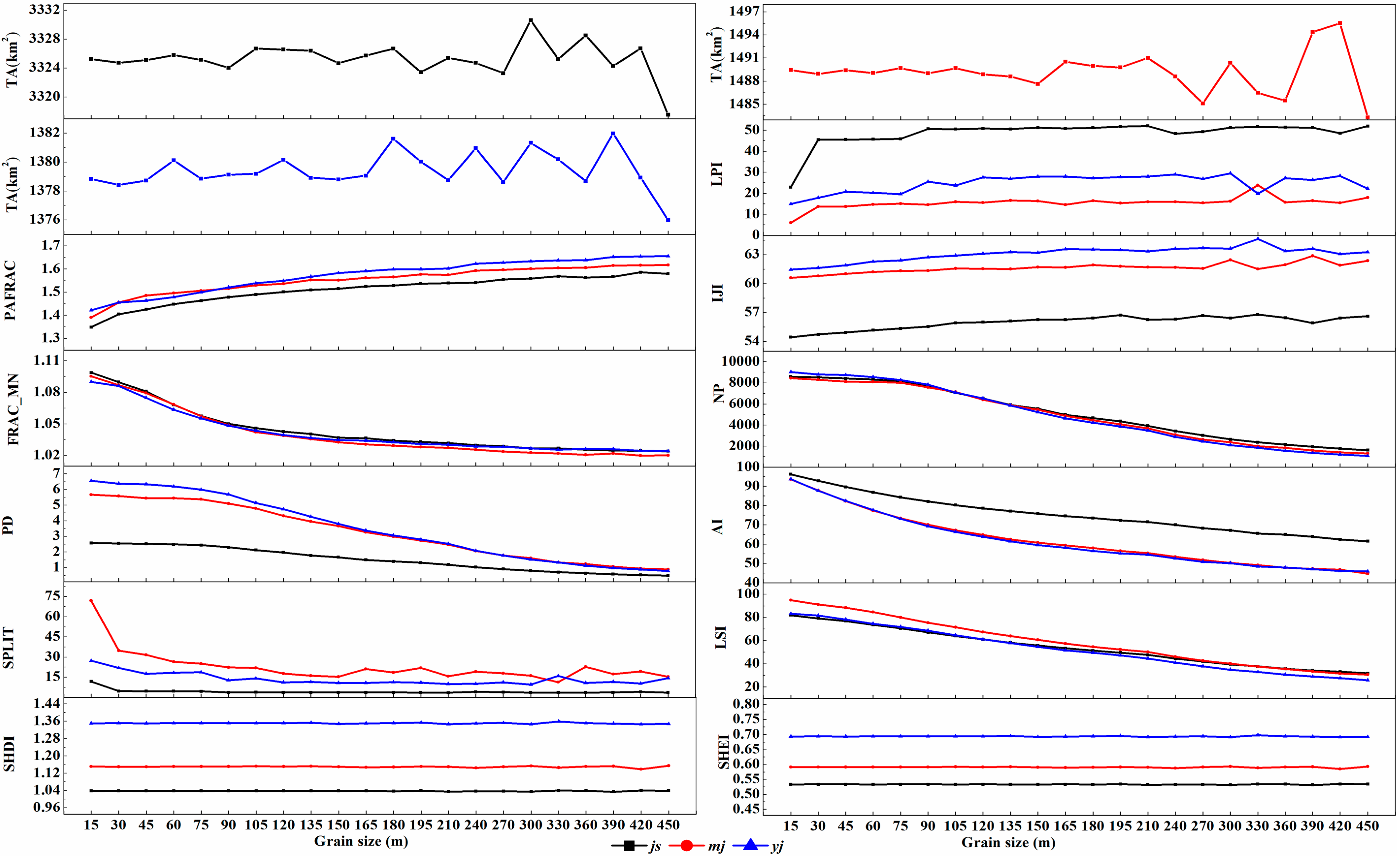
Figure 5.
Response curve of landscape metrics in class level.
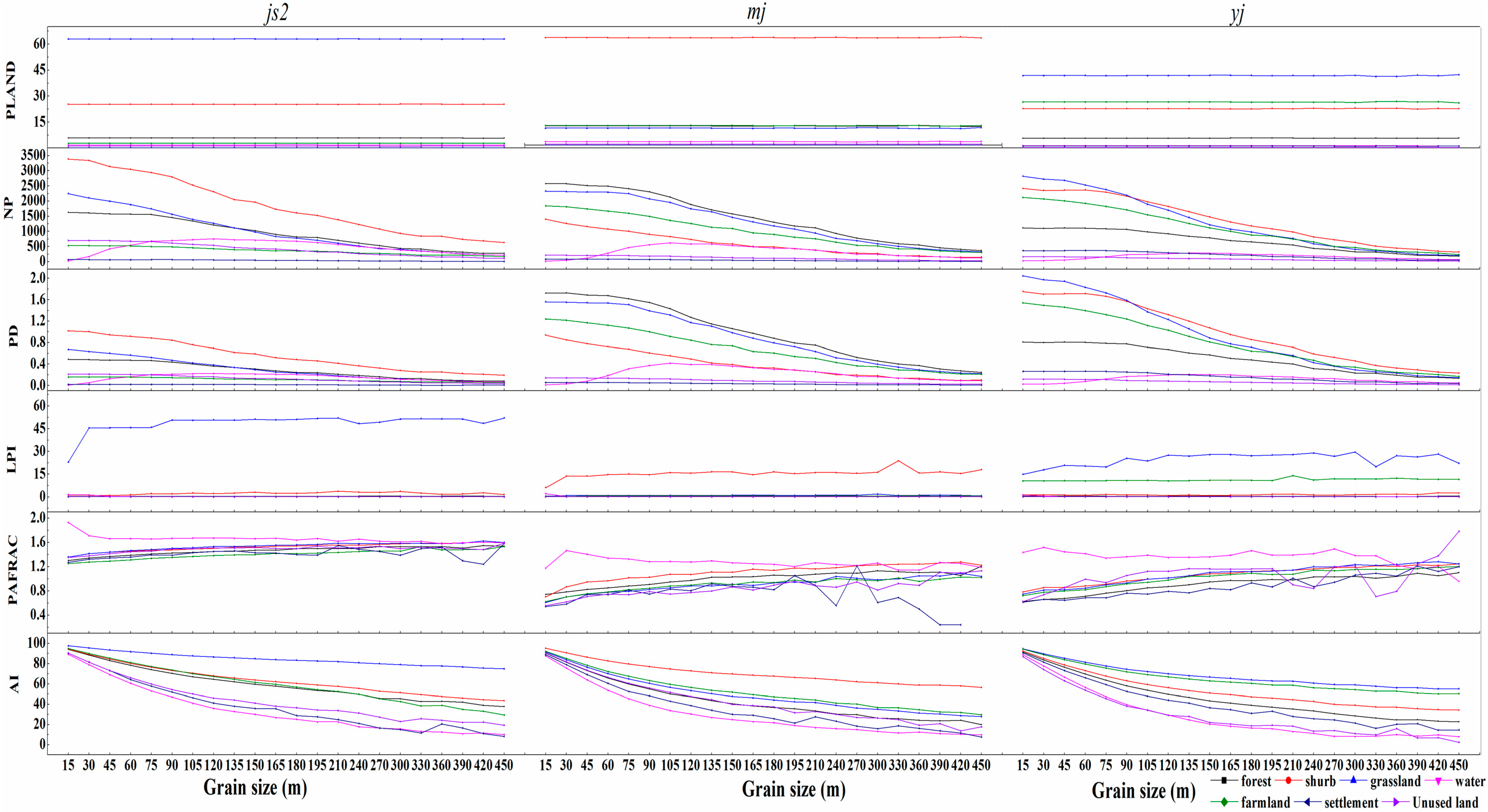
Figure 6.
The landscape metrics of the arid valleys at landscape level.

Figure 7.
The landscape metrics of the arid valleys at class level.

Table 1.
The area, length of river and boundary, mean DEM and mean slope of arid valleys.
| Basin Attributes | Area (km2) | The Length of River (km) | The Length of Boundary (km) | Mean DEM (m) | Mean Slope (°) |
|---|---|---|---|---|---|
| Dadu River | 1202.11 | 229.23 | 2845.23 | 2387.66 | 29.31 |
| Yuanjiang | 1378.76 | 187.50 | 1357.49 | 807.456 | 19.41 |
| Minjiang | 1489.17 | 404.41 | 3330.44 | 2377.56 | 30.46 |
| Anning River | 2693.62 | 677.71 | 2781.95 | 1649.52 | 15.10 |
| Yalong River | 3347.99 | 340.33 | 5734.65 | 2177.29 | 27.89 |
| Lancang River | 3457.13 | 586.16 | 4197.94 | 2572.87 | 29.68 |
| Nujiang | 4100.81 | 730.54 | 3312.10 | 2264.63 | 29.13 |
| Jinsha River | 15,390.53 | 2438.28 | 15,844.28 | 1927.06 | 25.58 |
Table 2.
Landscape pattern metrics, and their description, were chosen at landscape level.
| Metrics | Name | Description |
|---|---|---|
| Area and Edge metrics | Total Area (TA) | The area of the landscape |
| Largest Patch Index (LPI) | The proportion of the largest patch area | |
| Shape metrics | Perimeter-Area Fractal Dimension (PAFRAC) | Non-randomness or degree of aggregation for different patches |
| Fractal Index Distribution (FRAC_MN) | The shape complexity of patches, which approaches 1 for shapes with simple perimeters and 2 for complex shapes | |
| Aggregation metrics | Number of Patches (NP) | The number of patches |
| Patch Density (PD) | Number of patches per unit area | |
| Splitting Index (SPLIT) | The number of patches of a landscape divided into equal sizes keeping landscape division constant, express the separation degree of individual distribution in different | |
| Interspersion and Juxtaposition Index (IJI) | The measurement of evenness of patch adjacencies and the degree of intermixing of patch types | |
| Aggregation Index (AI) | The degree of aggregation of similar patches | |
| Landscape Shape Index (LSI) | The continuity and complex of landscape shape and the measurement of the perimeter-to-area ratio for the landscape as a whole. | |
| Diversity metrics | Shannon’s Diversity Index (SHDI) | Uncertainties and landscape heterogeneity of patches |
| Shannon’s Evenness Index (SHEI) | The degree of evenness of each patch in the area, which only consider the evenness of patch sizes, not the number of patches |
Table 3.
The estimation of response curves of landscape metrics in landscape level.
| Metrics | js2 | mj | yj | |||
|---|---|---|---|---|---|---|
| Curve Fitting | R2 | Curve Fitting | R2 | Curve Fitting | R2 | |
| TA | ||||||
| LPI | S function | 0.870 | S function | 0.790 | Cubic function | 0.746 |
| PAFRAC | Log function | 0.994 | Log function | 0.991 | Log function | 0.972 |
| FRAC_MN | Cubic function | 0.987 | Cubic function | 0.991 | Cubic function | 0.988 |
| NP | Exp function | 0.989 | Exp function | 0.987 | Exp function | 0.990 |
| PD | Exp function | 0.989 | Exp function | 0.987 | Exp function | 0.990 |
| SPLIT | S FUNCTION | 0.894 | S FUNCTION | 0.827 | S FUNCTION | 0.683 |
| IJI | Cubic function | 0.933 | Cubic function | 0.751 | Cubic function | 0.897 |
| AI | Cubic function | 0.999 | Cubic function | 0.998 | Cubic function | 0.998 |
| LSI | Cubic function | 0.999 | Cubic function | 0.998 | Cubic function | 0.998 |
| SHDI | ||||||
| SHEI | ||||||
Table 4.
The appropriate grain size of the landscape metrics by calculating in landscape level.
| Metrics | First Scale Domain | The Appropriate Grain Size |
|---|---|---|
| TA | The smaller, the better | |
| LPI | 30–90 m | 45–75 m |
| PAFRAC | 30–210 m | 45–195 m |
| NP | 60–105 m | 75–90 m |
| PD | 60–105 m | 75–90 m |
| SPLIT | 30–90 m | 45–75 m |
| IJI | 60–180 m | 75–125 m |
| AI | 45–240 m | 60–210 m |
| LSI | 45–105 m | 60–135 m |
| SHDI | <195 m | |
| SHEI | <195 m | |
| All | 60–90 m | 75 m |
Table 5.
The estimation of response curves of landscape metrics in class level.
| Metrics | js2 | mj | yj | ||||
|---|---|---|---|---|---|---|---|
| Patch | Curve Fitting | R2 | Curve Fitting | R2 | Curve Fitting | R2 | |
| PLAND | Forest | ||||||
| Shrub | |||||||
| Grass | |||||||
| Water | |||||||
| Farmland | |||||||
| Settlement | |||||||
| Unused land | |||||||
| NP | Forest | Cubic function | 0.995 | Cubic function | 0.997 | Cubic function | 0.992 |
| Shrub | Cubic function | 0.995 | Cubic function | 0.984 | Cubic function | 0.995 | |
| Grass | Cubic function | 0.991 | Cubic function | 0.994 | Cubic function | 0.990 | |
| Water | Cubic function | 0.518 | Cubic function | 0.490 | Cubic function | 0.399 | |
| Farmland | Cubic function | 0.984 | Cubic function | 0.996 | Cubic function | 0.996 | |
| Settlement | Cubic function | 0.950 | Cubic function | 0.985 | Cubic function | 0.977 | |
| Unused land | Cubic function | 0.996 | Cubic function | 0.990 | Cubic function | 0.987 | |
| PD | Forest | Cubic function | 0.995 | Cubic function | 0.997 | Cubic function | 0.992 |
| Shrub | Cubic function | 0.995 | Cubic function | 0.984 | Cubic function | 0.995 | |
| Grass | Cubic function | 0.991 | Cubic function | 0.994 | Cubic function | 0.990 | |
| Water | Cubic function | 0.519 | Cubic function | 0.490 | Cubic function | 0.400 | |
| Farmland | Cubic function | 0.984 | Cubic function | 0.996 | Cubic function | 0.996 | |
| Settlement | Cubic function | 0.950 | Cubic function | 0.985 | Cubic function | 0.977 | |
| Unused land | Cubic function | 0.996 | Cubic function | 0.990 | Cubic function | 0.987 | |
| LPI | Forest | S FUNCTION | 0.708 | Cubic function | 0.609 | Cubic function | 0.484 |
| Shrub | S FUNCTION | 0.458 | Cubic function | 0.487 | Cubic function | 0.524 | |
| Grass | Exp function | 0.547 | S FUNCTION | 0.499 | S FUNCTION | 0.551 | |
| Water | Power function | 0.909 | S FUNCTION | 0.408 | Exp function | 0.541 | |
| Farmland | Cubic function | 0.526 | Cubic function | 0.500 | Cubic function | 0.817 | |
| Settlement | Cubic function | 0.471 | Cubic function | 0.477 | Cubic function | 0.281 | |
| Unused land | Cubic function | 0.585 | Cubic function | 0.484 | Cubic function | 0.773 | |
| PAFRAC | Forest | Power function | 0.987 | Power function | 0.934 | Power function | 0.951 |
| Shrub | Power function | 0.995 | Power function | 0.974 | Power function | 0.966 | |
| Grass | Power function | 0.969 | Power function | 0.973 | Power function | 0.958 | |
| Water | Cubic function | 0.830 | Cubic function | 0.346 | Cubic function | 0.503 | |
| Farmland | Power function | 0.951 | Power function | 0.954 | Power function | 0.961 | |
| Settlement | Cubic function | 0.376 | Cubic function | 0.562 | Cubic function | 0.937 | |
| Unused land | Power function | 0.733 | Power function | 0.821 | Cubic function | 0.338 | |
| AI | Forest | Exp function | 0.984 | Exp function | 0.988 | Exp function | 0.987 |
| Shrub | Exp function | 0.984 | Exp function | 0.992 | Exp function | 0.988 | |
| Grass | Cubic function | 0.997 | Cubic function | 0.998 | Exp function | 0.989 | |
| Water | Exp function | 0.981 | Exp function | 0.963 | Exp function | 0.947 | |
| Farmland | Cubic function | 0.998 | Cubic function | 0.998 | Exp function | 0.989 | |
| Settlement | Exp function | 0.978 | Exp function | 0.980 | Exp function | 0.983 | |
| Unused land | Exp function | 0.988 | Exp function | 0.988 | Exp function | 0.969 | |
Table 6.
The appropriate grain size of the landscape metrics by calculating in class level.
| Metrics | Basin | First Scale Domain | The Appropriate Grain Size |
|---|---|---|---|
| PLAND | js2 | The smaller, the better | |
| mj | <125 m | ||
| yj | <135 m | ||
| NP | js2 | 60–135 m | 75–125 m |
| mj | 60–135 m | 75–125 m | |
| yj | 60–135 m | 75–125 m | |
| PD | js2 | 45–195 m | 60–180 m |
| mj | 45–195 m | 60–180 m | |
| yj | 45–195 m | 60–180 m | |
| LPI | js2 | <150 m | |
| mj | <150 m | ||
| yj | <120 m | ||
| PAFRAC | js2 | 45–135 m | 60–120 m |
| mj | 45–150 m | 60–135 m | |
| yj | 45–165 m | 60–150 m | |
| AI | js2 | 60–120 m | 75–105 m |
| mj | 45–180 m | 60–165 m | |
| yj | 60–195 m | 75–180 m | |
| All | 60–135 m | 75 m |
© 2017 by the authors. Licensee MDPI, Basel, Switzerland. This article is an open access article distributed under the terms and conditions of the Creative Commons Attribution (CC BY) license (http://creativecommons.org/licenses/by/4.0/).
Share and Cite
MDPI and ACS Style
Fang, S.; Zhao, Y.; Han, L.; Ma, C. Analysis of Landscape Patterns of Arid Valleys in China, Based on Grain Size Effect. Sustainability 2017, 9, 2263. https://doi.org/10.3390/su9122263
AMA Style
Fang S, Zhao Y, Han L, Ma C. Analysis of Landscape Patterns of Arid Valleys in China, Based on Grain Size Effect. Sustainability. 2017; 9(12):2263. https://doi.org/10.3390/su9122263
Chicago/Turabian StyleFang, Shu, Yonghua Zhao, Lei Han, and Chaoqun Ma. 2017. "Analysis of Landscape Patterns of Arid Valleys in China, Based on Grain Size Effect" Sustainability 9, no. 12: 2263. https://doi.org/10.3390/su9122263
Note that from the first issue of 2016, this journal uses article numbers instead of page numbers. See further details here.