Quantitative Analyses of Transition Pension Liabilities and Solvency Sustainability in China

School of Economics and Management, Beihang University, Beijing 100191, China
*
Author to whom correspondence should be addressed.
Sustainability 2017, 9(12), 2252; https://doi.org/10.3390/su9122252
Submission received: 17 October 2017
/
Revised: 19 November 2017
/
Accepted: 2 December 2017
/
Published: 6 December 2017
Abstract
:In the context of the aging population, the debt risk and solvency situation of China’s pension plan are of major concern for government and individuals. The aim of this paper is to project public pension liabilities and evaluate the solvency sustainability of China’s pension reform during transition periods. By using cohort component and actuarial models, transition debt and solvency sustainability are projected under the existing policy scenario and several sets of hypothetical policy scenarios. We find that the transition liabilities will peak in 2035 and the pension plan will become unsustainable in 2048 under existing policies. In the proposed scenario, postponing retirement age helps to maintain pension plan sustainability until 2083, but this option can’t solve the financial distress in the long run. Further, the transition pension debt will double in the peak moment if the retirement age is postponed for five years, which would pose a risk to the liquidity of the fund. Moreover, an increase to invest return can only improve the baseline solvency in short term. Sustainable options should be designed as composite reform measures, including retirement and investment adjustment.
1. Introduction
The issue of pension liability in China has aroused widespread concerns from research institutions and scholars at home and abroad. Especially after the 1997 structural reform, attention has been focused on the problems related to public pension liability and solvency sustainability during the transition period [1,2,3]. The goal of pension reform in China is to shift the financing mode from an unfunded system to a partially funded system (UF-PFF shift). With respect to actuarial theory, pension liability can be further subdivided into implicit debt and explicit debt in the UF-PFF shift. Implicit pension debt is the committed payment of the pension system, while explicit pension debt arises from the aging population and structural reform. Evidently, the UF-PFF shift will inevitably lead to the dominance of implicit pension debt. If the pension debt arising from the system transition is not handled properly, it will lead directly to an unsustainable pension plan. Thus, to ensure a stable shift in pension reform, it is necessary to measure the transition pension liabilities and the finances needed to repay it.
Franco (1995) clarified three main definitions of pension liabilities: accrued-to-date liabilities, current workers and pensioners’ liabilities, and open-system liabilities [4]. The calculation method of accrued-to-date liabilities assumes that a pension plan will terminate in the future and that the amount of accrued-to-date liabilities equals the present value of future pensions due to the past contributions of current workers. Furthermore, the calculations of current workers and pensioners’ liabilities assume that pension plans will remain sustainable until the last contributor dies and there are no new entrants. The amounts of current workers and pensioners’ liabilities equal the outcome of accrued-to-date liabilities plus the present value of future pensions due to future contributions of current workers. The calculation of open-system liabilities includes the present value of the pensions of new entrants, and the liabilities equal the current workers and pensioners’ liabilities plus the present value of pensions due to contributions of future generations [5]. However, with respect to an UF-PFF shift, the transition pension liability is not relevant to Franco’s definitions as it represents only the compensation for retirees who do not have individual pension accounts in the new system. Li Yang (2013) held that implicit pension debt is the sum of the current value of the fiscal gap in payments over time, a view considered from the perspective of the balance sheet [6]. Implicit debt is divided into two parts in Li Yang (2013)’s research, specifically, one arises from the structural reform of the pension system and the other stems from an aging population. Moreover, the definition of implicit pension debt in Li Yang (2013) is similar to the definition of open-system liabilities, and hence, his hierarchical computing method was conducive to a deeper understanding of the sources of pension liability and the repayment mechanism. Liu et al. (2015) constructed basic actuarial models that considered the expenditures of old retirees, middle retirees, and new retirees to forecast the liquidity gap of the social pooling account [7]. Their study, however, did not take into account differences in the insured population projections between the old and new pension systems. That said, there are no separate calculations for transition debt and annual expenditures. Tian and Zhao (2016) predicted the solvency sustainability of the social pooling for basic pensions on the basis of demographic projections [8], but they did not measure the transition debt that should have been paid by the social pooling pension fund. To compensate for the pension debt during the transition period, Wang, L. (2016) proposed that the government should increase the legal retirement age, reduce the pension replacement rate, and improve the investment yield of the pension fund [9]. However, his research did not evaluate how the pension debt would change as a result of the suggested policy options.
There are many studies that examine the effects of reform on pension schemes. Casamatta and Gondim (2009) considered the political support for parametric reforms of the pay-as-you-go pension scheme by using a continuous-time overlapping generation model [10]. Tabata (2015) estimated the effects of the reform of a defined benefit scheme to a defined contribution scheme using the framework of a two-period OLG model within endogenous growth [11]. Other relevant studies have examined the effects of a transition from the perspectives of population aging and fertility decline [12,13]. However, few empirical studies have investigated the transition liability and solvency sustainability from an unfunded system to a partially funded system, especially for the case of China. In this paper, we build on earlier work to estimate transition pension liabilities and solvency sustainability. Moreover, scenario analysis is implemented to evaluate the effect of the reform policy. The structure of this paper is organized as follows: Section 2 introduces the feature and system reform of China’s pension plan; Section 3 introduces the assumptions and data sources of actuarial evaluations; Section 4 describes the mathematical population model and summarizes the baseline results of the projections; the modelling of the transition pension debt and solvency sustainability are presented in Section 5; Section 6 analyses the transition debt and solvency sustainability from the perspective of alternative policy scenarios; and Section 7 concludes the contents of the previous six sections.
2. The Public Pension System in China
China’s public pension system for urban employees was established in early 1950s. Like most countries in the world, it was a pay-as-you-go system in the initial stage. As China moved toward a market economy, the transformation required a mobile workforce. Obviously, the unfunded pension system limited the portability of accrued benefits, and it was no longer suitable for economic growth. Further, the dramatic aging process of the population aggravated the financial burden of the pension scheme. In order to maintain the sustainability of the public pension system and promote economic development, China’s social security administration changed the pension system from an unfunded system to a partially funded system in 16 July 1997. Compared with the old pension system, the newly established scheme sets up two pension fund accounts (social pooling account and individual account) for each insured member. The social pooling part adopts the pay as you go system while the individual account part employs the funded system.
According to the Decision on Perfecting Enterprise Workers Basic Pension Insurance System (State Council No. 38 document) promulgated by the State Council of China, the insured employee contributed twenty percent of basic wage to the social pooling account and eight percent to the individual account every year [14]. Premiums paid by the insured for the social pooling account are not used for personal accumulation, but are mainly used to provide basic pensions for the retired elderly. The accumulated fund of individual account belongs to the insured employee, and the accumulation value determines the size of the individual pension when they retire. Since the insured workers in the old system did not have corresponding individual accounts, the pension benefits of this generation will be lower than the new entrants if calculated by the actuarial rules of the new system. To reflect the welfare and intergenerational equity of the pension plan, the Social Insurance Law of the People’s Republic of China promulgated in 2011 stipulates that the government should subsidize compensatory pensions to the transition generation. But in actuarial practice, the social pooling account bears the compensatory pension which should be paid by the government. Therefore, compensatory pensions are an extra liability for social pooling account during the transition period and they are also a latent factor of actuarial imbalance.
3. Actuarial Assumptions and Data Source
3.1. Actuarial Assumptions
- (1)
- Age assumptions: Age assumptions include entry age, normal retirement age, and survival limit age. Similar to previous studies, we suppose the entry age for insurance is 20 over the long term. Under the current legal provisions of China, male workers retire at 60, women retire at 50, and female cadres retire at 55 [8,15]. However, with the implementation of policies for gradually postponing the retirement age of employees, the retirement age will increase. Thus, in the benchmark scenario, the retirement age is set at 60 for men and 55 for women. Furthermore, since the 2010 to 2013 life table [16] is used in this article, for consistency, we chose the 105 as the survival limit age.
- (2)
- Sex ratio at birth: According to the National Population Development Plan (2016–2030), the future objective of gender ratio is set at 112 in year 2020 and 107 in year 2030 [17], while the generally accepted theoretical value is 102 to 107 [18]. Thus, with the reduction of gender preference, the gender ratio of Chinese urban infants is projected to be 107 boys to 100 girls in the evaluation period.
- (3)
- Contribution rate: According to the State Council No. 38 document, the contribution rate of the social pooling fund is set at 20 percent of the taxable payroll during the evaluation period [14].
- (4)
- Coverage rate: In terms of the development of human resources and social security in the 13th Five-Year plan, the coverage rate of the plan will reach 90 percent. Therefore, the coverage rate of urban employees’ pension plan is set to increase every year to reach 90 percent during the evaluation period.
- (5)
- Urbanization rate: According to the data released by the National Bureau of Statistics, the urbanization rate of the population has increased from 17.92 percent in 1978 to 56.10 percent in 2015. The urban development report of China indicates that the urbanization rate of China will increase to more than 75 percent by 2050. Hence, the urbanization rate is set to increase year by year to reach 75 percent.
- (6)
- Urban employment rate: According to the Statistical Yearbook of China, the ratio of urban employment in the past year has remained at approximately 85 percent. Thus, this paper assumes that the future urban employment rate will remain at this level during the prediction interval.
- (7)
- The social pooling replacement rate: According to the State Council No. 38 document, the total replacement rate of an urban employee’s contributed payroll tax for more than 35 years is set at 59.2 percent of the social average wage, and the social pooling replacement rate is set at 35 percent of the social average wage [14].
- (8)
- Return rate: Referring to past study [8] and recent changes, we assume that the interest rate under the benchmark scenario is 0.03.
- (9)
- Growth rate of the social average wage: To predict the future pension debt, the future growth rate of social average wage is needed. However, based on the forecast of historical time series, the predicted value is inaccurate. Therefore, we refer to the research [19] to set 8 percent as the average wage growth benchmark.
- (10)
- Growth rate of pension benefit: According to the latest statistics announcement from the Ministry of Human Resources and Social Affairs (MHRSA), the pension growth rate was approximately 6.5 percent in 2016 and 5.5 percent in 2017. Therefore, in the predictable future, we assume the pension growth rate will remain at approximately 6 percent.
- (11)
- Actuarial parameters in the old pension system: The actuarial parameters in the old system include replacement rate () of the old retiree, the adjustment proportion (d) and the calculation coefficient (R) of the transition pension for the middle retiree. Based on reference to previous research [19], we suppose equals 75 percent, d equals 0.6, and R equals 1.3 percent.
3.2. Data Source
- (1)
- Life table: this research uses the China Life Insurance Mortality Table (2010–2013) [16] to obtain the survival rate of the insured population. Compared to the second set of life tables issued in 2005, life expectancy of the third set of tables for men and women, respectively, is 79.5 and 84.6; an increase of 2.8 and 3.7.
- (2)
- Initial population: the transition equations of population projections use age-sex specific population data of 2013 as the initial population vector. The data are obtained from China’s population and employment statistics yearbook [20].
- (3)
- The initial accumulated net assets of pension funds are obtained from a statistical bulletin on human resources and social security development [21]. The accumulated social pooling pension fund equals the total fund less the assets of individual accounts that have been partially repaid.
4. Projection of Population
4.1. Projection of the Insured Population in the Old Pension System
We primarily forecast the insured population in the old pension system. According to the previous research, the population that retired before 1997 is defined as the old retiree, and the population that worked before 1997 and retired after 1997 is defined as the middle population [22]. The middle population can be further divided into middle retiree and middle worker. The difference is that middle retiree is older than normal retirement age while middle worker is younger than normal retirement age in year t. To analyze the trend of the transition pension debt scale over time, we first predict the population size of insured old retirees, middle retirees and middle workers and investigate the transformation among the three groups.
Based on the statistics from the Ministry of Labour and Social Security and National Bureau of Statistics, by the end of 1997, the basic old-age insurance system covered 86.71 million employees (i.e., middle workers) and 25.33 million retirees (i.e., old retirees). The population of middle retirees after 1997 can be calculated based on their survival probability. To obtain the age-sex-specific populations of old retirees and middle workers in 1997, we use 1% of the sample survey data of the 1997 national population to calculate the urbanization rate, age structure and gender ratio. Accordingly, based on the demographic structure data of 1997, the next t year’s age-specific population can be forecasted using a survival transition equation that is expressed as follows:
where denotes the number of people aged x at time t and denotes the survivorship proportion of age group x at 1997 to age group x + t − 1997 at time t. On the basis of the third set of life table data, the survival probability after t years is obtained as follows:
Figure 1 presents the projected population tendency of old retiree, middle retiree and middle worker. From the picture, it is evident that the populations of old retiree and middle worker exhibit a decline trend. Due to death, the old retiree group will decrease to zero in 2047. The middle worker, who will transition to middle retiree upon reaching retirement age, will decrease to zero in 2036. The population of middle retiree experiences a tendency to first increase and then decrease. Before year 2036, the growth of ‘middle retiree’ is mainly driven by the inflow of ‘middle worker’. When all middle workers reach the normal retirement age, the population of the middle retiree will reach a maximum of 67.7 million, after which the population of middle retiree is affected mainly by death and hence will be attenuated in 2081.
4.2. Projection of Total Insured Population in the New Pension System
In the long run, the insured population under the new system is dynamic and open. We first use the cohort component method to project the age-sex specific population. Then, based on the forecasted population and relative proportion parameters, we forecast the number of insured employees and beneficiaries.
4.2.1. Projection of Age-Sex-Specific Population
The cohort component method is widely employed to forecast the structure of populations [23,24,25]. The key to this approach is to construct a Leslie matrix model based on the Euler-Lotka equation. A Leslie matrix is a discrete, age-structured model of population growth, it stems from the works of Bernardelli, Lewis, and Leslie [26,27,28]. In the field of demography, a Leslie matrix is used to forecast the changes of population over a period of time. Before constructing the transition equation, we first compute the age specific fertility rate of baby boys and baby girls. As we have assumed in Section 3.1, the sex ratio at birth, denoted as , equals 107 boys to 100 girls in the evaluation period. Thus, the proportion of baby boys in new born babies is and the proportion of baby girls in new born babies is . The annual age specific fertility rate of baby boys and baby girls can be calculated as:
where denotes the age specific fertility rate of baby boys in year ; denotes the age specific fertility rate of baby girls in year ; denotes age specific fertility rate in year ; denotes the sex ratio at birth. The indexes , , , and denote male, female, time, and age. The transition equations are modelled through iterative equations that encompass demographic elements, specifically, initial age-specific population vector, age-specific fertility rate and survival rate, as follows:
Since the demographic elements (population, fertility rate and survival rate) are divided into 19 age groups (0–4, 5–9, 10–14, …, 80–84, 85–89, 90+) in the basic data, the time cycle is set to be 5 years in the population transfer process. Also, the time cycle of Leslie matrix is set to 5 years. Based on the assumption of a five-year cycle, the women of childbearing age will experience five reproductive opportunities. Thus, the number of births per year () needs to be adjusted to the number of births in five years () in the transition equation. Because most of the members in the social pension scheme are employees of state-owned enterprises, the migration rate of these employees can be disregarded in the long run. These transition equations can be conveniently written in matrix form as:
or in more compactly form as
Using the Leslie matrix operations, the cohort component method makes it possible to forecast populations a few years in the future. That is, to project the population in year , the initial population vector is multiplied by the Leslie matrix until :
where denotes the population of age class in year t, denotes the survival rate of an age-sex class; denotes the age-specific fertility; is the population vector, and is the Leslie matrix. The indexes t, s, m, f, and n refer to year, age, male, female, and the maximum age group respectively.
Figure 2 presents the result of the seventy-year population projection. From the picture, it is evident that total population will experience a growth trend in years 2018 to 2028 and then decrease rapidly after that. Accordingly, the forecasted value of the total population will increase from 1388 million in 2018 to 1408 million in 2028 and then decline to 838 million in 2088.
4.2.2. Projection of Insured Employees in the New Pension System
The insured employees in the new system contribute payroll taxes to the social pooling account every year. To calculate the annual contributions, the population of insured employees is projected based on the projected age-sex specific population. The forecasting model of insured employees is presented as
where denotes the population of insured employees in year t; denotes the urbanization rate of population in year ; denotes the ratio of urban employment in year ; denotes the coverage ratio of urban employee’s pension plan in year . The indexes m, f, and s refer to male, female and age respectively.
Figure 3, which displays the population of insured employees indicates that the number of insured employees will increase during the initial period and then begin a continual decline. The forecasted population of insured employees will decrease from 314 million in 2023 to 152 million in 2088.
4.2.3. Projection of Insured Beneficiaries in the New Pension System
The insured beneficiaries receive scheduled benefits from the social pooling account, and thus the population of beneficiaries is comprised of new arrivals who have attained retirement age and survived retirees from previous years. The forecasting model of insured beneficiaries is presented as
where denotes the population of pension beneficiaries in year t; denotes the urbanization rate of population in year t; denotes the ratio of urban employment in year t; denotes the coverage ratio of urban employee’s pension plan in year t. The indexes m, f, and s refer to male, female and age respectively. Figure 4, which presents the projected population of pension beneficiaries, indicates that with the acceleration of the aging population, the number of retired employees will continue to increase. Moreover, due to the retirement of the baby boomers, the retirement population will increase rapidly between 2018 and 2023. Hence, the forecasted value of pension beneficiaries will increase from 91.99 million in 2018 to 185.11 million in 2088.
5. Modeling Transition Pension Liabilities and Pension Fund Solvency
5.1. Modeling Transition Pension Liabilities
5.1.1. Modeling Transition Pension Liability of Old Retiree Group
Due to the structural reform of the pension plan, the transition liability of the old retiree generation originated from the social security administration’s additional subsidies. Assume that the x-year-old old retiree retired at , the social average wage level is , the growth rate of the social average wage is , the retirement age is r, and the pension replacement rate of old retiree is . Accordingly, the average wage of the old retiree in the last year before retirement is calculated as
According to the official data released by Ministry of Human Resources and Social Security of China, the pension growth rate was d ratio of the average social wage growth rate before 2007, and the pension growth rate remained at 10 percent in 2007–2015 [29]. After that, the pension growth rate remains at the assumed level . The x-year-old old retiree receives a pension benefit in the first year of retirement, and the amount of the pension at the beginning of t is , which can be calculated as
By formula (15), the x-year-old old retiree at the beginning of t year receives a pension benefit. Wang (2000) assumed that the transitional pension of old retiree is about 50% of the basic pension [30]. After offsetting the pension rights accumulated in the pay-as-you-go system, the total transition pension liability of the old retiree group equals 0.5 percent of the pension multiplied by the age-specific population , which is calculated as
Because the old retirees were retired before 1997, the lower limit of their age should be . If the lower limit age of the old retiree exceeds the upper age limit age in the life table, it means that the old retiree group are no longer alive, and hence, this group can be ignored when calculating pension debt.
5.1.2. Modeling Transition Pension Liability of Middle Retiree Group
The transition pension liability of the middle retiree reflects the government’s commitment to subsidize the middle retiree group during the period. Accordingly, this subsidy is also called the transition pension and it can be calculated as
where denotes the indexed average payment wage; e is the entry age for pension insurance; R is the computation coefficient; (x – e − (t − 1997)) denotes the compensation years. Taking into account the difference in the calculation of the indexed average payment wages of different provinces, we simplified the indexed average payment wage as the social average wage a year before retirement. Thus, the transition pension of the x-year-old middle retiree is calculated as
The age range of the middle retiree is , and the total transition pension liability of the middle retiree can be calculated as
The total transition pension debt is measured by aggregating the liabilities of the old retiree and the middle retiree groups
where denotes the total transition pension liabilities in year ; denotes the transition pension liabilities of old retiree in year ; denotes the transition pension liabilities of middle retiree in year .
5.2. Modeling Social Pooling Pension Fund Solvency
The annual accumulated net asset, or fiscal gap when it is negative, is a common measure to evaluate the solvency of the pension fund. The social pooling account receives payroll taxes and interest income. In turn, scheduled benefits are paid from the social pooling account. To assess the solvency of the social pooling fund contributed from the taxable payroll, the government’s subsidy is not considered in the evaluation. Thus, the annual accumulated net asset at the end of a given year is numerically equal to the net asset at the beginning of the year, plus payroll taxes, plus interest income, less scheduled benefits and less transition debt, and the administrative expenses are neglected in the long run. Accordingly, the actuarial model is expressed as
where denotes the contributions from payroll taxes in year ; denotes the scheduled benefits in year ; denotes the value of net assets (reserve fund) in year ; denotes the contribution ratio of taxable payroll in year ; denotes the social average wage in year ; denotes the population of insured employees in year ; denotes the replacement ratio of the social pooling pension in year ; denotes the population of pension beneficiaries in year ; and denotes the interest rate.
6. Scenario Analysis
Scenario-based analyses are widely used to evaluate uncertain shocks and alternative policies. In this section we mainly use the scenario analysis method to assess the impact of potential reform measures on transition pension liability and solvency sustainability. For a given pension system, the main economic and demographic assumptions that determine pension liabilities and solvency sustainability include interest rate, real wage growth, survival probabilities, and retirement age. In particular, we consider changes to retirement age and investment return in the scenario analysis.
6.1. Scenario Analysis of Transition Pension Liability
According to the existing retirement policy, the benchmark age for retirement is 60 for men and 55 for women, which is no longer suitable for the development of the aging society. To illustrate how the delayed retirement policy affect the transition liabilities, we present two scenarios: the baseline scenario and the delayed retirement scenario. The baseline scenario assume the employees retire at the existing benchmark age, while the delayed retirement scenario propose a retirement age delay of five years. Because the old retiree group had retired before 1997, their pension benefit will not be affected by delaying retirement age. However, the case for the middle retiree group is different. Since the delayed retirement policy mainly affects the retirement age of middle workers, the middle retiree group are most affected by postponing retirement. Firstly, we analyze the projected population of the middle retiree group in the baseline and delayed retirement scenarios. Figure 5 provides the projections of the middle retiree population in two scenarios.
The middle retiree population in the baseline scenario will increase from 34.99 million in 2018 to 67.74 million in 2036. When the middle worker group is fully converted into retirees in 2036, the number of middle retirees will reach its maximum. Compared with the baseline level, the population of middle retirees in the delayed retirement scenario is less than the baseline population in the years 2018 to 2041, and the population will be equal in the two scenarios until the youngest middle worker reaches the delayed retirement age, in 2041. After which the population of middle retirees is affected only by death and hence will be attenuated in 2081.
As introduced in model (17), the middle retiree receives an unchanged transition benefit every year. The total amount is only relevant to the population and the indexed average payment wage, which are two factors that have different effects on the total debt at different times. Figure 6, which presents the total transition debt of the middle retiree group, reveals that the transition debt in the delayed retirement scenario increases rapidly up to 2044, with a maximum of two times the baseline level. This indicates that the population of middle retirees dominated the debt amount in the initial stage, but that over time the indexed average payment wage and compensation years (x − e − (t − 1997)) have a major effect on the total amount of the transition debt.
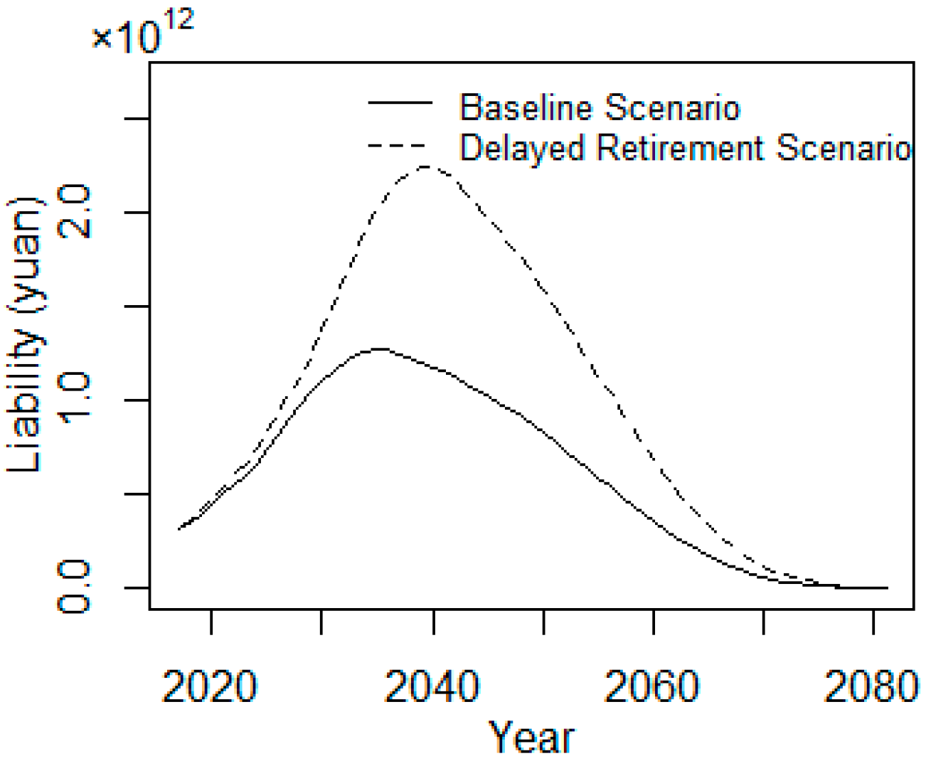
As introduced in model (20), the total amount of transition pension debt is estimated by aggregating the liabilities of the old retiree and the middle retiree groups. Because the transition debt of the middle retiree group has a high percentage of total debt, the projected trend of total debt is similar to the transition liability of the middle retirees, as shown in Figure 7. The total transition debt in the baseline scenario increases from 437 billion yuan in 2018 to 1286 billion yuan in 2035. The total transition debt in the delayed retirement scenario increases from 453 billion yuan in 2018 to 2051 billion yuan in 2044, with a maximum of two times the baseline total debt in the peak moment. So, this debt risk arising from delayed retirement should not be ignored when drawing up funding plans.
6.2. Scenario Analysis of Solvency Sustainability
There are different ways to measure the solvency sustainability of the pension plan. W. Cheng et al. (2004) presented three types of measures to assess the financial sustainability of the combined OASDI trust funds: (1) annual balances, income rates, and cost rates; (2) trust fund ratios; and (3) open group unfunded obligation [31]. Tian and Zhao (2016) presented the accumulated net asset to evaluate pension fund sustainability [8]. Compared with the indicators introduced by W. Cheng et al. (2004), the accumulated net asset is more applicable to assess China’s pension plan. If the accumulated net asset value goes below zero in the assessment period, the pension fund becomes unsustainable. Thus, this research used the accumulated net assets as the main indicator to evaluate solvency sustainability. Based on the actuarial model (23) and the population forecasting models, a comparison of solvency sustainability in the baseline, postponing retirement, and increasing return rate scenarios is conducted.
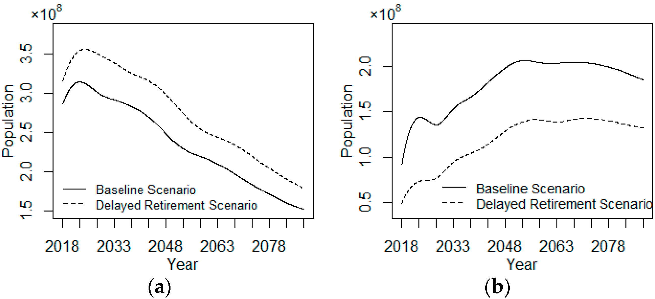
We first compare the projection of insured employees and retirees in the baseline and postponing retirement scenario. Then, we evaluate the solvency sustainability of pension plan in the alternative scenarios. Figure 8a presents the population of insured employees in each of the two cases, both of which experience a declining trend in the context of aging. With the implementation of the delayed retirement policy, the predicted value of insured employees increases by 15% on average during the horizon 2018–2078. Figure 8b, which displays the population of insured retirees in two scenarios, indicates that the predicted trends are nearly the same. Compared with the projection in the baseline scenario, the population of insured retirees in the postponing retirement scenario decreases by 35% on average during the horizon 2018–2078.
Next, we examined impact of postponing retirement age on solvency sustainability. As presented in Figure 9, the trend of accumulated net assets first increases slowly and then decreases. The baseline solvency of the pension fund becomes unstainable in 2048, while the solvency in the postponing retirement scenario maintains sustainability until 2083. Compared with the average retirement age in the world, the retirement age of insured employees in China is relatively earlier, and a retirement age of five years later can effectively improve the solvency of the pension scheme. However, the implementation of the delayed retirement policy is only effective in the short term (2018–2083) and it is not effective to change the downward trend of the accumulated net assets in the long run.
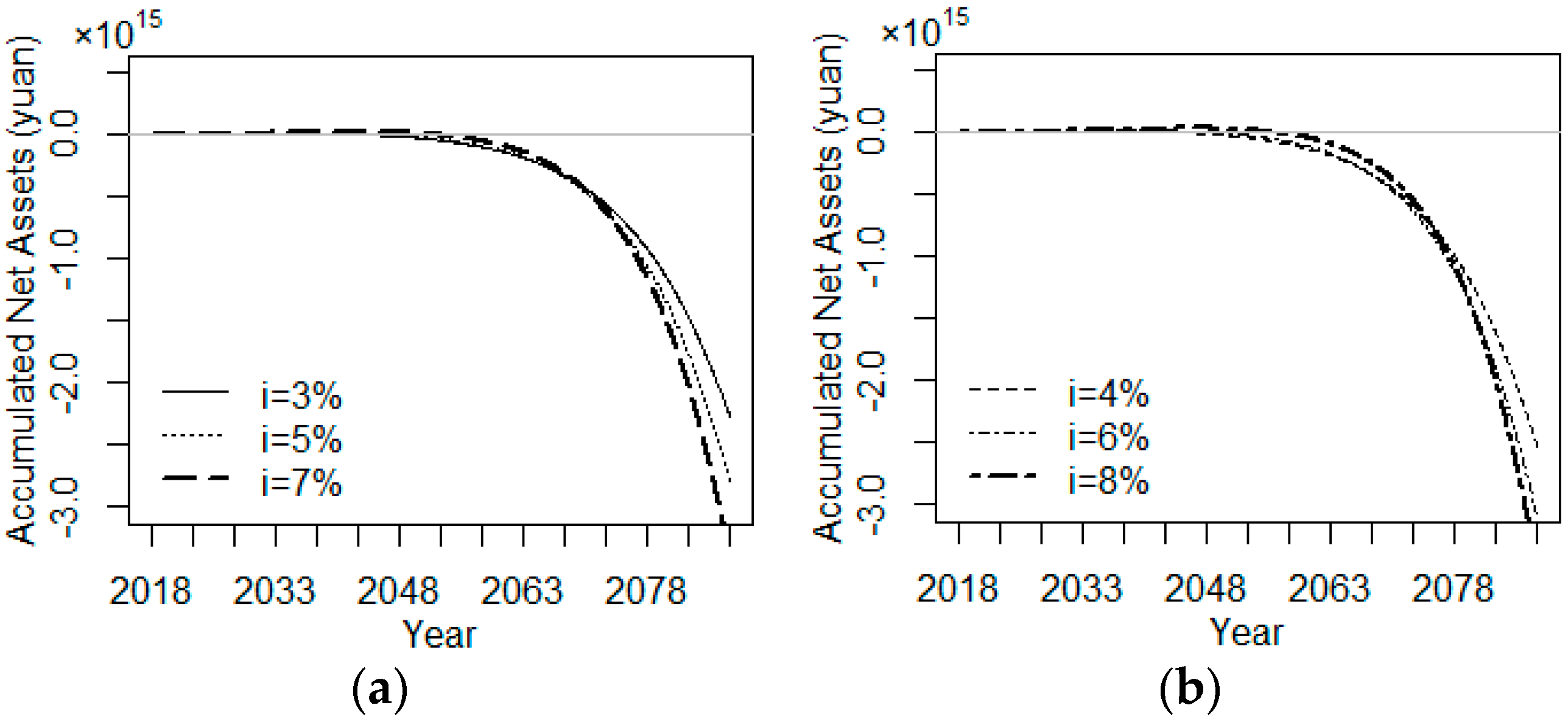
As Rauh and Novymarx (2011) pointed out, the expected return on pension plan assets is typically around 8% in the major international financial institutions [32]. However, China’s social pension fund calculates earnings based on fixed deposit interest rates, about 3%. In order to solve the problem of the low yield of the pension fund, on 1 April 2015, the State Council of China executive meeting decided to appropriately expand the scope of pension fund investment, expand the fund investment to local government bonds, equity investment, trust loan investment, interbank deposit certificate and so on. According to the Investment Management Regulations for Old-age Insurance Pension Fund issued by the State Council in 17 August 2015, the pension fund of each province will gradually entrust to the National Council for Social Security Fund of China for investment operation. As reported by the annual report of Social Security Fund in 2016, the average annual yield of the Social Security Fund managed by the National Council for Social Security Fund had reached 8.37% during the whole investment operation period [33]. Therefore, we assume that the upper limit of the yield is 8%, and the corresponding scenario analysis is implemented by assuming the return rate increase from 3% to 8% while the other assumptions remain unchanged. Figure 10 illustrates the sensitivity tests of return rate under the baseline retirement scenario.
In the existing retirement policy, the general trend of pension fund solvency will remain the same regardless of the increase in the return rate by several percentage points. It can be concluded that the pension plan can’t alleviate financial burden simply by increasing investment yield. Table 1 gives the test results of return rate increases under the baseline retirement scenario. It can be seen clearly that with the increase of the return rate, the timing of the financial gap is delayed for 5–15 years. When the yield is below four percent, the pension plan will have a funding gap between years 2043–2048. However, a one percentage point increase in the return rate would delay the gap time for five years when the return rate exceeds six percent.
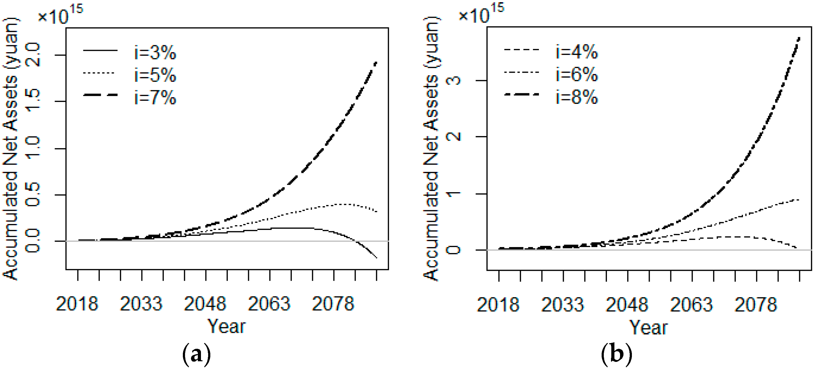
Figure 11 presents the sensitivity tests of return rate under the delayed retirement scenario. As can be seen, the pension plan will maintain sustainability throughout the evaluation period, except the interest rate equals three percent. The accumulated net assets of the pension fund will increase first and then decrease when the return rate is below five percent, whereas the cumulative asset will continue to increase when the yield exceed five percent.
Table 2 gives the test results of return rate increases under the delayed retirement scenario. When the return rate is three percent, the accumulated net asset will reach a maximum of 149 trillion in 2068; the accumulated net asset will reach a maximum of 227 trillion in 2073 when the return rate is four percent; and the accumulated net asset will reach a maximum of 393 trillion in 2078 when the return rate is five percent. When the return rate exceeds five percent, the accumulated net asset will keep increasing during the evaluation period, and a one percentage point increase in return rate would raise the total asset significantly.
Together, these results suggest that the proposed policy options will significantly improve the solvency sustainability. Specifically, to ensure the pension scheme maintains financial sustainability in the long run, the yield of pension fund investment should be more than five percent under the delayed retirement option. However, we should also evaluate the effects of relevant policies on social welfare and economic growth to choose an optimal strategy.
7. Conclusions
In this paper, we highlight the importance of evaluating pension debt and solvency sustainability of a pension plan during a transition period. Based on the projected population and relative economic variables, we forecast transition pension liability and solvency sustainability for the years 2018 to 2088. Moreover, evaluations of potential reform options are measured using the scenario-analysis method. Our empirical results indicate that due to the unique actuarial model of transition pension liability, the amount of the transition pension debt will double in the peak moment if the retirement age is delayed by five years, hence increasing the risk of budget shortfalls. Furthermore, compared to the solvency sustainability under the baseline scenario, postponing retirement age could help to maintain the pension plan as sustainable in the years 2018–2083, but this situation will not last long due to the low return of pension assets. In addition, it should be noted that the mortality trends are estimated based on the historical mortality rates from the 2010–2013 life table, which will underestimate the impact of longevity risk. If the mortality trends are projected using a dynamic model, the transition liabilities will be larger and the pension fund will face a greater gap.
The sensitivity tests of the return rate in the baseline scenario and delayed retirement scenario indicate that, rather than relying solely on a postponed retirement age to maintain sustainability, combined policy options are more effective in improving solvency sustainability and they exhibit less distortion. Based on the simulated results, to ensure the pension plan is sustainable in the long term, the minimum objective of the social security sector reform is to postpone retirement age for 5 years and hold the investment yield above 5%. However, as the policy options that we have designed are not yet fully realistic, in future studies we will consider the impact of changing the actuarial parameters on solvency sustainability.
Acknowledgments
This work was supported by Contracts (71571007, 71333014) from National Natural Science Foundation of China. We would like to thank Qiyao Luo and Yazhou Gao for their help. However, the opinions expressed here do not necessarily reflect the policy of National Natural Science Foundation.
Author Contributions
Yueqiang Zhao established the model and implemented in R; Yali Liu and Junzhang Hao contributed analysis and discussion; Manying Bai modified the grammar approved the final manuscript.
Conflicts of Interest
The authors declare no conflict of interest.
References
- Feldstein, M. Social security pension reform in China. China Econ. Rev. 1999, 10, 99–107. [Google Scholar] [CrossRef]
- Yin, J.Z.; Lin, S.; Gates, D.F. Social Security Reform: Options for China; World Scientific Publishing Co. Pte. Ltd.: Singapore, 1999; pp. 223–259. ISBN 978-981-02-4104-9. [Google Scholar]
- Dorfman, M.C.; Holzmann, R.; O’Keefe, P.; Wang, D.; Sin, Y.; Hinz, R. China’s Pension System: A Vision; World Bank: Washington, DC, USA, 2013; pp. 15–75. [Google Scholar] [CrossRef]
- Franco, D. Pension Liabilities—Their Use and Misuse in the Assessment of Fiscal Policies; Working Paper; Directorate General for Economic and Financial Affairs, European Commission: Brussels, Belgium, 1995. [Google Scholar]
- Holzmann, R. Financing the Transition to Multipillar; Working Paper; World Bank: Washington, DC, USA, 1998. [Google Scholar]
- Yang, L.; Xiao, Z. China’s National Balance Sheet 2013: Theory, Methodology and Risk Assessment; China Social Sciences Publishing House: Beijing, China, 2013; pp. 214–215. ISBN 978-7516138199. [Google Scholar]
- Liu, X.; Zhang, Y.; Fang, L.; Li, Y.; Pan, W. Reforming China’s Pension Scheme for Urban Workers: Liquidity Gap and Policies’ Effects Forecasting. Sustainability 2015, 7, 10876–10894. [Google Scholar] [CrossRef]
- Tian, Y.; Zhao, X. Stochastic Forecast of the Financial Sustainability of Basic Pension in China. Sustainability 2016, 8, 46. [Google Scholar] [CrossRef]
- Wang, L. Actuarial model and its application for implicit pension debt in China. Chaos Solitons Fractals 2016, 89, 224–227. [Google Scholar] [CrossRef]
- Casamatta, G.; Gondim, J.L.B. Reforming the Pay-As-You-Go Pension System: Who Votes for it? When? FinanzArchiv Public Financ. Anal. 2011, 67, 225–260. [Google Scholar] [CrossRef]
- Tabata, K. Population Aging and Growth: The Effect of Pay-as-You-Go Pension Reform. FinanzArchiv Public Financ. Anal. 2015, 71, 385–406. [Google Scholar] [CrossRef]
- Fanti, L.; Gori, L. Fertility and PAYG Pensions in the Overlapping Generations Model. J. Popul. Econ. 2012, 25, 955–961. [Google Scholar] [CrossRef] [Green Version]
- Artige, L.; Cavenaile, L.; Pestieau, P.; SSRN. The Macroeconomics of PAYG Pension Schemes in an Aging Society. 2014. Available online: http://dx.doi.org/10.2139/ssrn.2438689 (accessed on 10 October 2017).
- The State Council of China. Available online: http://www.gov.cn/zhuanti/2015-06/13/content_2878967.htm (accessed on 19 September 2017).
- Yang, D.U.; Wang, M. Demographic Ageing and Employment in China; ILO Employment Working Paper No. 57; Employment Sector, International Labor Office: Geneva, Switzerland, 2010. [Google Scholar]
- China Insurance Regulatory Commission. Available online: http://www.circ.gov.cn/web/site0/tab5213/info4054990.Htm (accessed on 12 October 2017).
- The State Council of China. Available online: http://www.gov.cn/zhengce/content/2017-01/25/content_5163309.htm (accessed on 19 October 2017).
- Jiang, Y.Y. Construction of Intergenerational Accounting System and Social Insurance System Reform in China; Peking University Press: Beijing, China, 2015; p. 22. ISBN 978-7301254592. [Google Scholar]
- Zhang, Y.B.; Liu, Z.-X.; Bai, M.-Y.; Luo, Q.-Y. China’s Basic Implicit Pension Debt Trends Analysis—Based on the Improved Actuarial Calculation Model Empirical Study. Chin. J. Manag. Sci. 2013, 21, 40–49. [Google Scholar]
- National Bureau of Statistics of the People’s Republic of China. Available online: http://www.stats.gov.cn/tjsj/ndsj/2014/indexch.htm (accessed on 12 September 2017).
- Ministry of Human Resources and Social Security of the People’s Republic of China. Available online: http://www.mohrss.gov.cn/.2014 (accessed on 15 October 2017).
- Tao, M.; Qi, Y. An actuarial analysis on the implicit pension debt in social pension system of China. Popul. J. 2011, 4, 68–74. [Google Scholar] [CrossRef]
- Thomas, J.R.; Clark, S.J. More on the cohort-component model of population projection in the context of HIV/AIDS: A Leslie matrix representation and new estimates. Demogr. Res. 2011, 25, 39–101. [Google Scholar] [CrossRef] [PubMed]
- Tian, F. Demographic Probabilistic Forecast Method and Its Application. Northwest Popul. J. 2011, 5, 9–13. [Google Scholar] [CrossRef]
- Pânzaru, C. On the Sustainability of the Romanian Pension System in the Light of Population Declining. Procedia Soc. Behav. Sci. 2015, 183, 77–84. [Google Scholar] [CrossRef]
- Bernardelli, H. Population Waves. J. Burma Res. Soc. 1941, 31, 1–18. [Google Scholar] [CrossRef]
- Lewis, E.G. On the Generation and Growth of a Population. Sankhya Indian J. Stat. 1942, 6, 93–96. [Google Scholar] [CrossRef]
- Leslie, P.H. Some Further Notes on the Use of Matrices in Population Mathematics. Biometrika 1948, 35, 213–245. [Google Scholar] [CrossRef]
- Ministry of Human Resources and Social Security of China. Available online: http://www.mohrss.gov.cn/SYrlzyhshbzb/shehuibaozhang/zcwj/yanglao/ (accessed on 9 August 2017).
- Wang, X.J. China’s Pension System and Its Actuarial Evaluation; Economic Science Press: Beijing, China, 2000; pp. 172–177. ISBN 978-7505820289. [Google Scholar]
- Cheng, A.W.; Miller, M.L.; Morris, M.; Schultz, J.P.; Skirvin, J.P.; Walder, D.P. A Stochastic Model of the Long-Range Financial Status of the OASDI Program; Annual Report; Pub. No. 11-11555; Office of the Chief Actuary, U.S. Social Security Administration: Washington, DC, USA, 2004.
- Rauh, J.D.; Novymarx, R. Policy Options for State Pension Systems and Their Impact on Plan Liabilities. J. Pension Econ. Financ. 2011, 10, 173–194. [Google Scholar] [CrossRef]
- National Council for Social Security Fund of the People’s Republic of China. Available online: http://www.ssf.gov.cn/cwsj/ndbg/201706/t20170612_7277.html (accessed on 20 October 2017).
Figure 1.
Population trend of ‘old retiree’, ‘middle retiree’ and ‘middle worker’ (2018–2081).
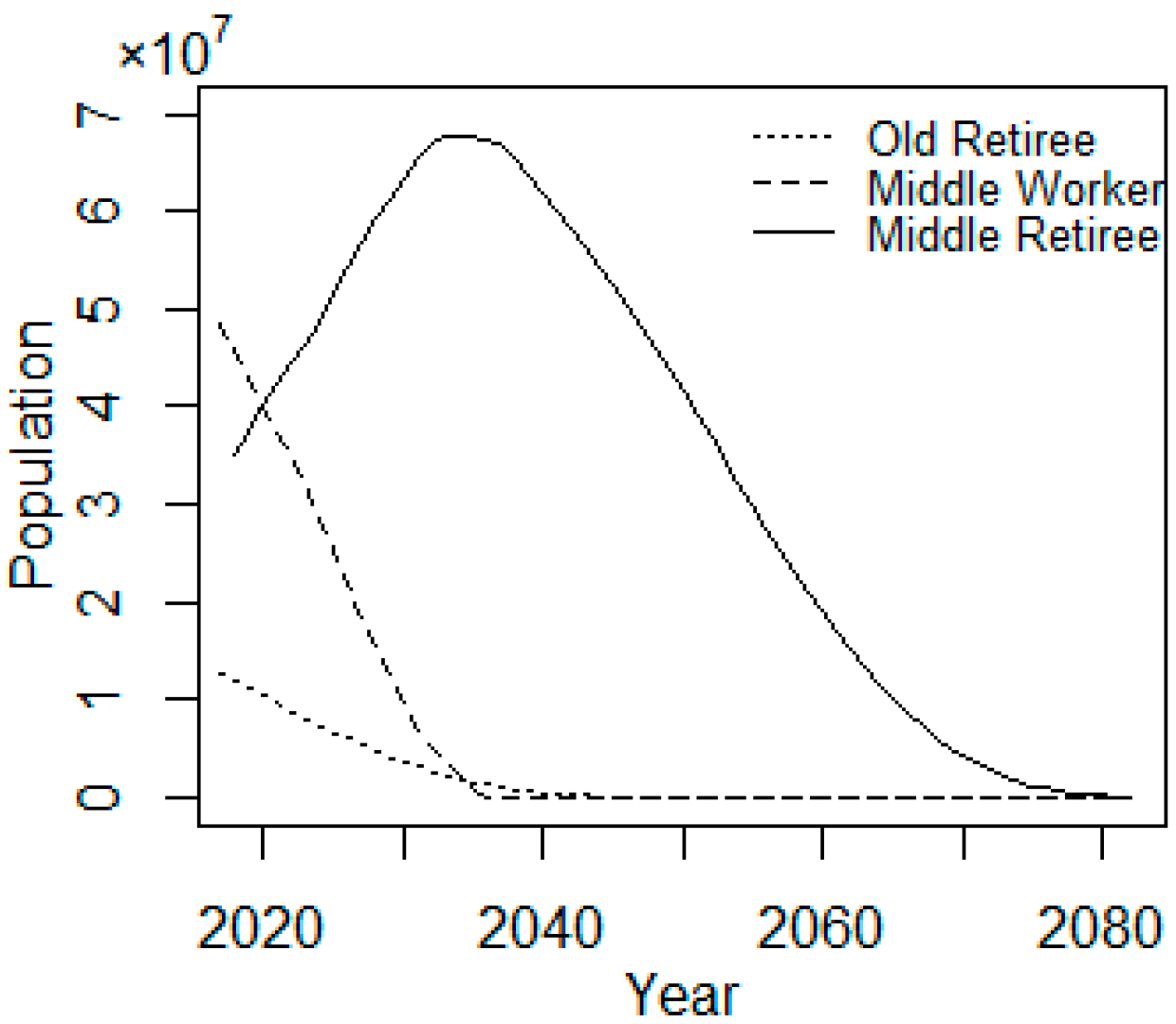
Figure 2.
Projection of total population.
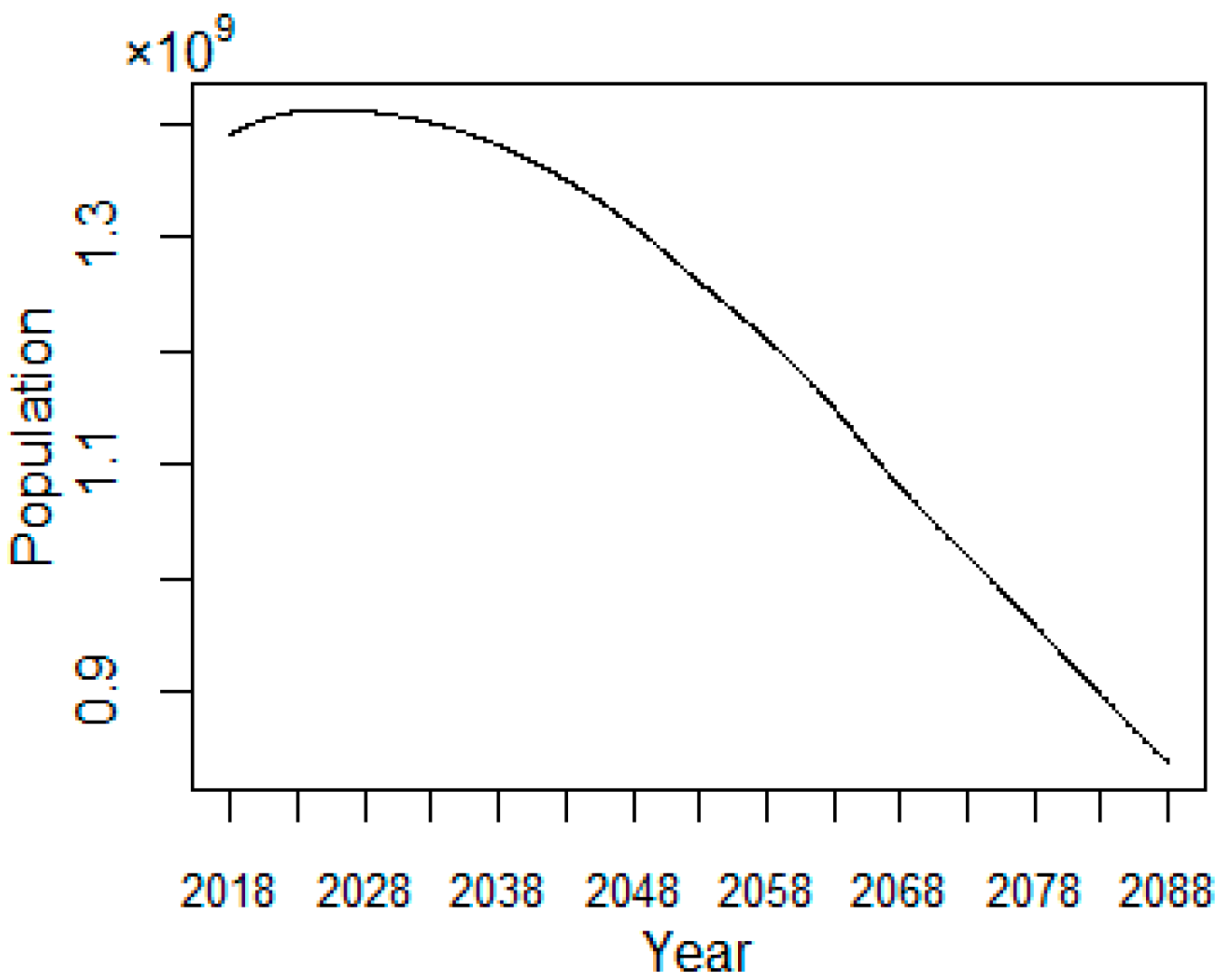
Figure 3.
Projection of insured employees.

Figure 4.
Projection of insured beneficiaries.
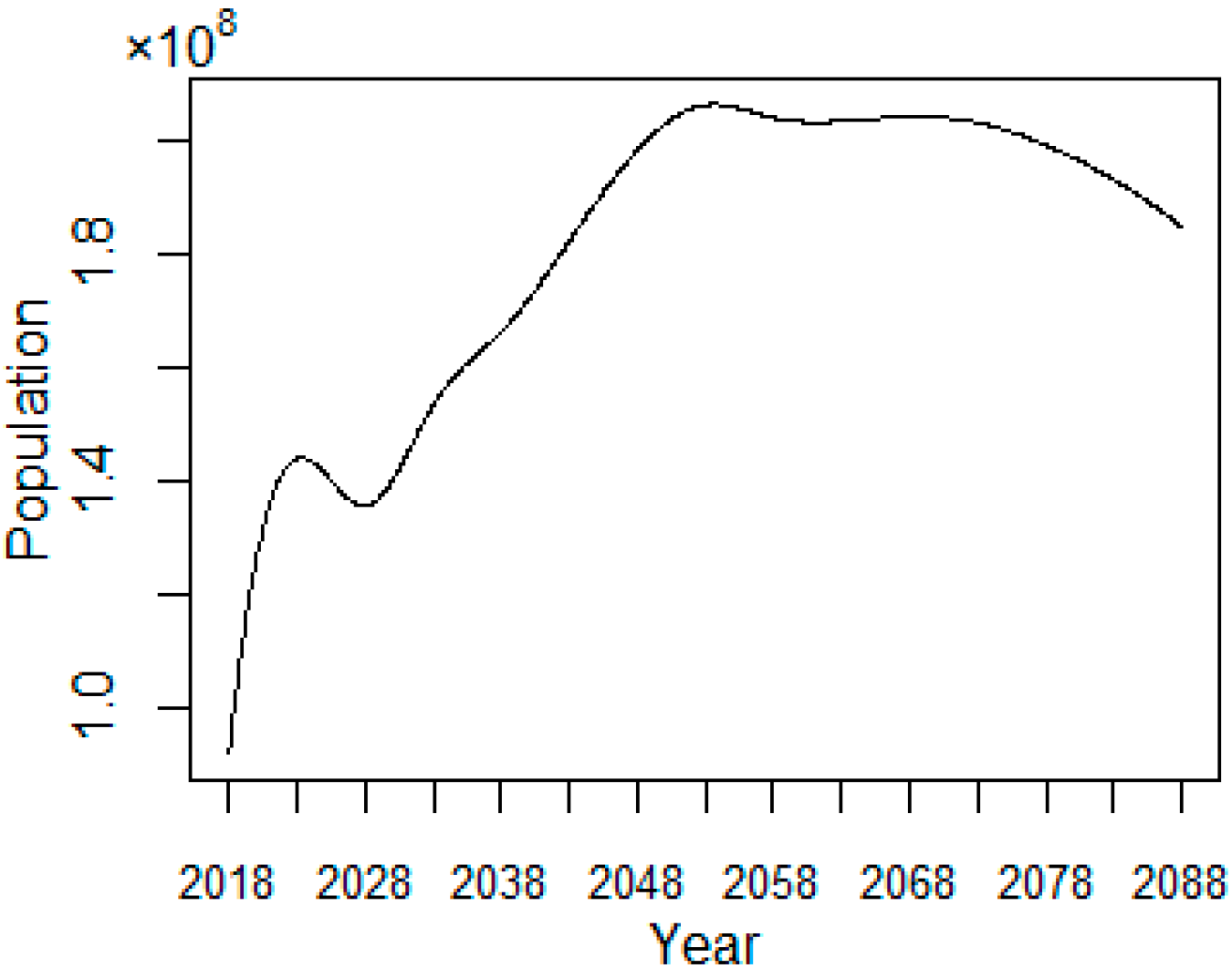
Figure 5.
Comparison of projected middle retiree group.

Figure 6.
Transition pension liability of middle retiree group.

Figure 7.
Total transition pension liability.
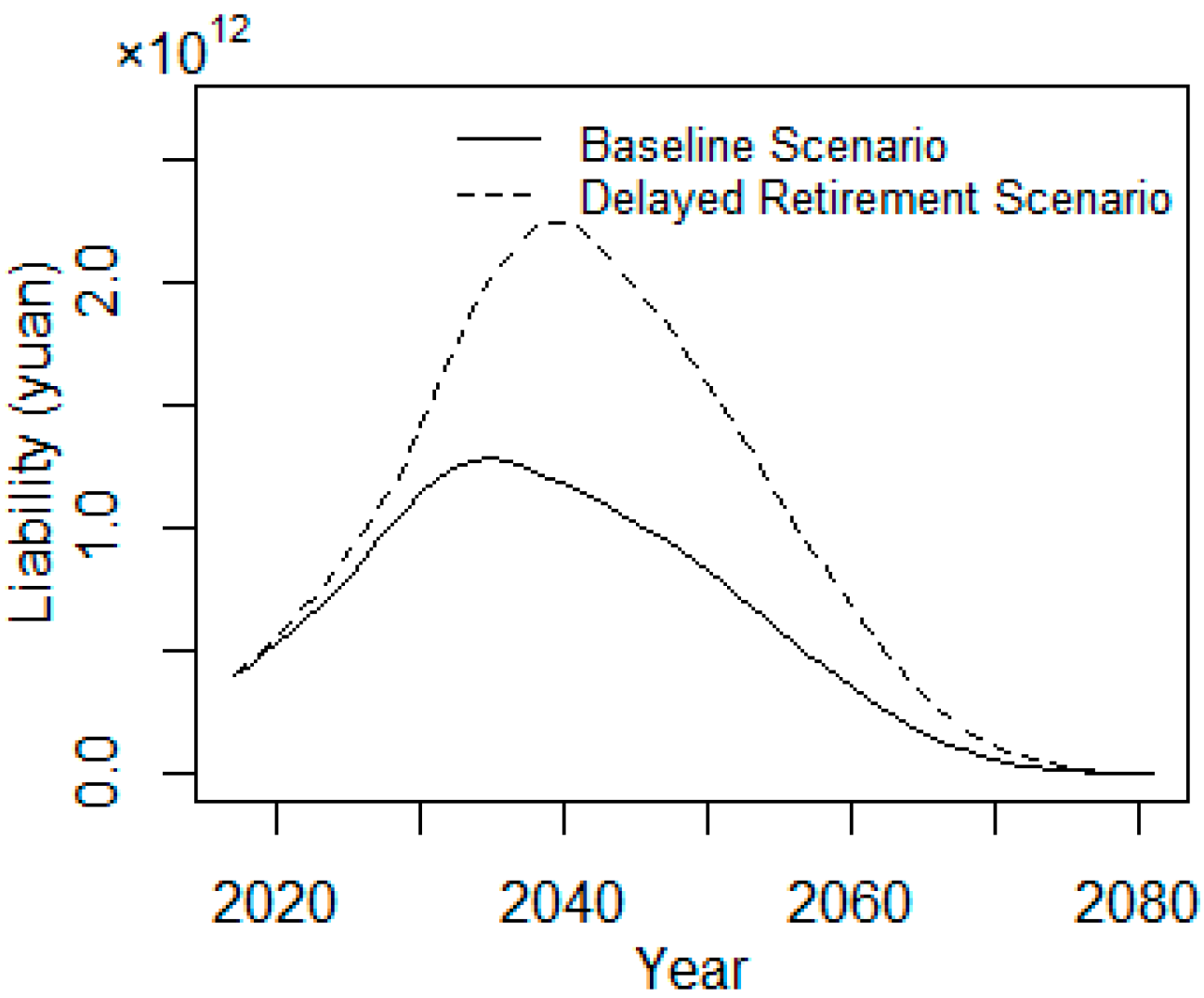
Figure 8.
(a) Projection of insured employees; (b) Projection of insured retirees.

Figure 9.
Projection of pension fund solvency.
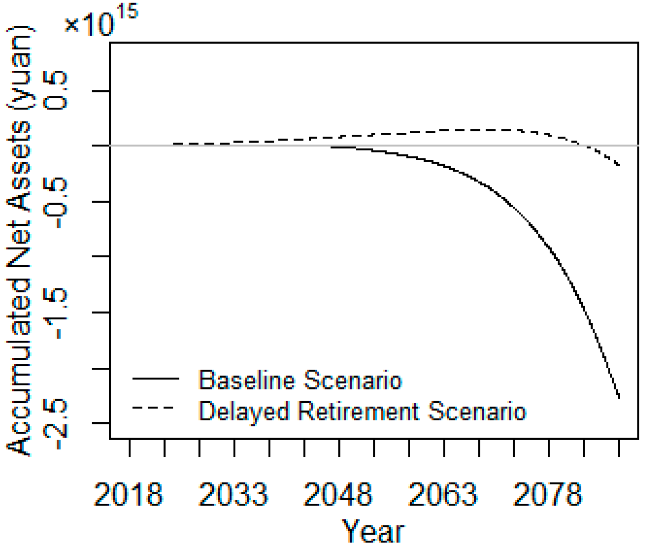
Figure 10.
(a) i = 3%, 5%, 7%; (b) i = 4%, 6%, 8% (the baseline retirement scenario).

Figure 11.
(a) i = 3%, 5%, 7%; (b) i = 4%, 6%, 8% (the delayed retirement scenario).

Table 1.
Test results of accumulated asset under baseline scenario (trillion).
| Year | i = 3% | i = 4% | i = 5% | i = 6% | i = 7% | i = 8% |
|---|---|---|---|---|---|---|
| 2018 | 4.43 | 4.57 | 4.71 | 4.86 | 5.02 | 5.18 |
| 2023 | 6.09 | 6.52 | 6.97 | 7.46 | 7.99 | 8.57 |
| 2028 | 8.49 | 9.35 | 10.30 | 11.40 | 12.60 | 14.00 |
| 2033 | 9.91 | 11.40 | 13.20 | 15.30 | 17.80 | 20.70 |
| 2038 | 9.63 | 12.10 | 15.00 | 18.70 | 23.10 | 28.50 |
| 2043 | 4.79 | 8.31 | 12.80 | 18.60 | 26.00 | 35.50 |
| 2048 | −10.60 | −6.08 | 0.18 | 8.73 | 20.30 | 36.00 |
| 2053 | −42.90 | −37.90 | −30.30 | −18.80 | −2.00 | 22.40 |
| 2058 | −95.70 | −92.20 | −84.70 | −71.20 | −48.90 | −13.30 |
| 2063 | −182.00 | −183.00 | −179.00 | −166.00 | −139.00 | −90.30 |
| 2068 | −325.00 | −337.00 | −342.00 | −337.00 | −310.00 | −247.00 |
| 2073 | −558.00 | −590.00 | −618.00 | −631.00 | −615.00 | −543.00 |
| 2078 | −920.00 | −993.00 | −1060.00 | −1120.00 | −1140.00 | −1070.00 |
| 2083 | −1470.00 | −1610.00 | −1760.00 | −1900.00 | −2000.00 | −1980.00 |
| 2088 | −2270.00 | −2530.00 | −2810.00 | −3110.00 | −3370.00 | −3480.00 |
Table 2.
Test results of accumulated net asset under delayed retirement scenario (trillion).
| Year | i = 3% | i = 4% | i = 5% | i = 6% | i = 7% | i = 8% |
|---|---|---|---|---|---|---|
| 2018 | 6.02 | 6.16 | 6.30 | 6.45 | 6.61 | 6.77 |
| 2023 | 11.60 | 12.10 | 12.70 | 13.25 | 13.88 | 14.56 |
| 2028 | 19.80 | 21.10 | 22.60 | 24.14 | 25.88 | 27.80 |
| 2033 | 30.30 | 33.00 | 36.10 | 39.57 | 43.57 | 48.12 |
| 2038 | 44.00 | 49.00 | 54.90 | 61.83 | 69.97 | 79.57 |
| 2043 | 61.70 | 70.40 | 80.80 | 93.47 | 108.87 | 127.65 |
| 2048 | 81.50 | 95.60 | 113.00 | 135.06 | 162.68 | 197.55 |
| 2053 | 101.00 | 122.00 | 150.00 | 186.86 | 234.24 | 296.30 |
| 2058 | 118.00 | 150.00 | 194.00 | 251.61 | 330.11 | 436.94 |
| 2063 | 138.00 | 184.00 | 248.00 | 337.21 | 463.41 | 642.58 |
| 2068 | 149.00 | 213.00 | 306.00 | 441.25 | 639.82 | 933.51 |
| 2073 | 141.00 | 227.00 | 359.00 | 558.24 | 865.41 | 1340.12 |
| 2078 | 98.90 | 213.00 | 393.00 | 682.08 | 1149.78 | 1906.14 |
| 2083 | 6.39 | 149.00 | 392.00 | 804.68 | 1504.52 | 2690.08 |
| 2088 | −173.00 | 4.81 | 325.00 | 898.00 | 1930.00 | 3770.00 |
© 2017 by the authors. Licensee MDPI, Basel, Switzerland. This article is an open access article distributed under the terms and conditions of the Creative Commons Attribution (CC BY) license (http://creativecommons.org/licenses/by/4.0/).
Share and Cite
MDPI and ACS Style
Zhao, Y.; Bai, M.; Liu, Y.; Hao, J. Quantitative Analyses of Transition Pension Liabilities and Solvency Sustainability in China. Sustainability 2017, 9, 2252. https://doi.org/10.3390/su9122252
AMA Style
Zhao Y, Bai M, Liu Y, Hao J. Quantitative Analyses of Transition Pension Liabilities and Solvency Sustainability in China. Sustainability. 2017; 9(12):2252. https://doi.org/10.3390/su9122252
Chicago/Turabian StyleZhao, Yueqiang, Manying Bai, Yali Liu, and Junzhang Hao. 2017. "Quantitative Analyses of Transition Pension Liabilities and Solvency Sustainability in China" Sustainability 9, no. 12: 2252. https://doi.org/10.3390/su9122252
Note that from the first issue of 2016, this journal uses article numbers instead of page numbers. See further details here.