The Catalan Economy towards the New European Energy Policy: Through Accounting of Greenhouse Emission Multipliers

Abstract

The aim of this paper is to study the effect that implementing the agreement signed by the European Union at the end of 2008 will have on reducing greenhouse gas emissions in Catalonia. Emission multipliers and the impact of reducing emissions by 10%, in sectors not covered by the EU ETS (EU Emissions Trading System) and reducing those that are covered by 21%, are analysed. More specifically, the effects on the endogenous income of the multiplier model (production, factorial and private income) is studied, while reducing and increasing endogenous income and the decomposition of emission multipliers into open, own and circular effects is analysed to include the different channels of the process of generating CO₂ equivalent emissions. The empirical application is for the Catalan economy and uses economic and environmental data for the year 2001. The results show that increases in greenhouse gas emissions will essentially depend on the account that receives the exogenous inflow in demand. Greenhouse gas emissions in Catalonia are affected very differently at the sectoral level and the effects of production activities, factors of production and consumption on air pollution are very heterogeneous. The analytical approach used in this paper provides interesting results that can help to design and implement policies to reduce emissions.

1. Introduction

For years, modern societies have been characterised by the ever-increasing requirement that a high standard of welfare must be compatible with a high level of environmental protection and that it should be possible to sustain the demand for natural resources, while at the same time absorbing pollution and decreasing negative impacts on the planet. The economic model currently in force in industrialised countries, combined with increasing population figures in developing countries and these people’s desire to attain a higher standard of welfare, has often led to the inappropriate consumption of natural resources, causing serious environmental problems. Consequently, the greatest problem facing the planet now is climate change.

It should be remembered that carbon dioxide emissions and those of other greenhouse effect gases occur naturally and are an essential pre-condition for life on Earth, since they retain the heat from the Sun in our atmosphere. Artificial emissions produced by humans add carbon dioxide to the atmosphere, leading to greater global warming. This is the phenomenon known as climate change. (according to the Intergovernmental Panel on Climate Change, the contribution made by Working Group I to the Fourth Assessment Report (Paris, 2007) concludes that global warming is unequivocal and can be attributed with over 90% certainty to human activity. The average global temperature on the Earth’s surface has increased by 0.74 °C in the last hundred years. The surface temperature in the last ten years of the twenty-first century is predicted to be between 1.8 and 4.0 °C higher than in the last twenty years of the twentieth century. Atmospheric CO₂ concentrations have increased by 35.36% since the preindustrial era. All of this has had a significant negative impact on ecosystems and socioeconomic systems across the planet, including considerable effects in southern Europe.)

Finding solutions to mitigate the effects of climate change requires sustained strategies, implemented in both the medium- and long-term, that meet the requirements of each sector or economic system. Finding appropriate solutions and putting them into practice is a formidable task and very few of those proposed so far have prospered, resulting in underestimations of the consequences of the problem or it being pushed aside by putting other subjects, such as the economic crisis, into the media spotlight.

The magnitude of the problem is very real and if we do not find an effective way to resolve the problem, the consequences for humanity may be disastrous. It is, therefore, vitally important that viable policies and measures are conceived to be able to react to the situation within an appropriate period as a continuous interactive process. Only if we manage to put effective policies to reduce emissions of greenhouse effect gases into action will we be able to improve air quality and quality of life in general for both humans and all other species living on the planet. What is more, such policies would enable us to save energy and to improve the quality and reliability of our infrastructures, in addition to making companies more competitive with greater potential to export highly technical goods and services without inflicting so much damage on the natural environment.

Bearing in mind that CO₂ emissions are closely related to economic growth, it is interesting to note that greenhouse gas emissions decreased in the European Union (EU) by an average of 2.5% between 2010 and 2011, although they increased in several other countries (according to the reports “Approximated EU greenhouse gas inventory: early estimates for 2011 [1]“ and ‘Greenhouse gas emission trends and projections in Europe 2012 [2]”).

The lowered greenhouse gas emissions in the EU may be largely due to the financial crisis, as consumers have moderated their use of electricity and private vehicles and merchant shipping has declined. Similarly, high petrol prices, drastically reduced construction activity, decreased car sales, lower demand for electricity and natural gas and higher unemployment have contributed to this reduction (according the report “Greenhouse Gas Emissions in Spain 1990–2012 [3].

In Spain in 2012, greenhouse gas emissions fell by 1.9% compared with the previous year. However, comparing figures with those from 1990, the base year for the Kyoto Protocol, emissions in fact increased by 18.7%. In the period 2008–2012, Spain’s emissions rose by an average of 24.5% relative to the base year, thus exceeding the Kyoto Protocol target by over 15%. Although in 2012 greenhouse gases in Spain were reduced, it continues to be one of the industrialised countries that has increased emissions most since 1990. In Catalonia, greenhouse gas emissions have increased by 47% in the last 15 years, 10% above the increase established by the Kyoto Protocol, which aimed to reduce emissions growth by 37% relative to the base year 1990 (according to the Department of Climate Change in Catalonia, as in the rest of the world, there has been an increase in the average annual temperature, in this case of 0.24 °C per decade for the period 1950–2011, with a higher increase in the summer (up to 0.35 °C per decade). Changes in precipitation, however, are far more difficult to establish clearly, particularly in our Mediterranean region of highly variable seasonal and inter-annual rainfall and its irregular spatial distribution. However, a 5.4% per decade reduction in summer rainfall has been observed for the period 1950–2011.)

At the end of 2008, the EU adopted an integrated policy for climate change and energy, which includes various ambitious objectives for 2020. The intention is to take Europe towards a sustainable future, with an economy that is low in carbon and has more rational consumption levels; the aim is to reduce greenhouse gas emissions in the Union by 20% relative to 1990 levels by 2020 (30% of other developed countries have agreed to effect similar reductions and the more advanced developed countries have agreed to contribute based on their responsibilities and capabilities). This agreement also stipulates that energy consumption must be reduced by 20% through improved energy performance and that 20% of our energy demands must be supplied by renewable energies (see the report “European council adopts climate-energy legislative package [4]).

This agreement establishes that the most contaminating sectors, which have been identified by the EU emissions trading system (EU ETS), have to cut their emissions by 21% compared to 2005, while other sectors, such as transport and household, have to reduce emissions by 10%. To prevent the sectors that contaminate most from moving their factories outside the EU, thereby leading to massive job losses, 100% of emission rights are awarded to companies that exceed certain thresholds. With respect to countries outside the ETS system, each country is assigned an objective relative to its GDP (in this way, the richest countries would have to reduce greenhouse gases by up to 20% and the poorest countries would be able to increase them by up to 20%).

In the case of Spain, 20% of the energy consumed must come from renewable sources by 2020. Furthermore, emissions must be reduced by 10% relative to 2005 levels (reference year) in sectors that are not covered by the ETS, such as transport, household, agriculture and farming and residues and sectors that are covered by the ETS must reduce their emissions by 21% by the same year.

The COP23 UN Climate Summit 2017, recently held in Bonn (Germany), was attended by 194 countries, 9200 government representatives and more than 16,000 participants. The talks in Bonn were mainly centred around establishing specific regulations to implement the 2015 Paris Climate Agreement. The Paris Agreement was a political milestone in that the countries involved set a firm goal to keep global warming below 2 °C. However, experts agree that this ambitious objective will be even more difficult to reach after President Trump’s rejection of the Paris Agreement and his threat to withdraw from the deal altogether in 2020 unless it was renegotiated.

Fijian Prime Minister and COP23 President, Frank Bainimarama, said that the COP23 had been a success, “especially given the challenge to the multilateral consensus for decisive climate action” and that, “We have done the job we were given to do, which is to advance the implementation guidelines of the Paris Agreement and prepare for more ambitious action in the Talanoa Dialogue of 2018”. (The CPO 23 also released the Talanoa dialogue design for facilitative dialogue at the next conference (Katowice, Poland) in 2018 where countries will, “take stock of the collective efforts of Parties in relation to progress towards the long-term goal and reiterate their collective commitment to make a wise decision for the collective good: new and more ambitious NDCs by 2020 to achieve the temperature goal of the Paris Agreement” (i.e., to keep global warming below 2 °C) or, if possible to limit the increase in temperature to a maximum of 1.5 °C (i.e., in regards to the pre-industrial era).)

He also added that, “We all leave Bonn having notched up some notable achievements, including our Ocean Pathway, the historic agreement on agriculture, an action plan on gender and a decision that benefits local communities and indigenous peoples. We have also secured more funding for climate adaptation and […] we have taken the important next step to ensure that the Adaptation Fund shall serve the Paris Agreement. We have also launched a global partnership to provide millions of climate-vulnerable people the world over with affordable access to insurance”.

A key outcome of the Bonn conference was The Powering Past Coal Alliance made up of more than twenty countries and other sub-national players advocating for phasing out coal and oil-fired electricity production by 2030 for OECD countries and by 2050 for the rest of the countries. The Alliance has warned not only of the serious effects to health burning coal has (such as respiratory diseases), but also the impact it has on global warming. The declaration signed by the Alliance members notes that, “… more than 800,000 annual deaths are related solely to coal burning” and that coal phase-out is “one of the most important steps” governments can take to tackle climate change and to meet their commitment to limit the increase in temperature to a maximum of two degrees with regard to pre-industrial values. Led by the United Kingdom and Canada, the Alliance also has the support of Italy, France, Holland, Austria, and Mexico. However, the group has caused a division within the EU as Germany, Poland and Spain, with their varying degrees of coal dependency, have yet to join (in Spain this year, coal will provide 18% of the electricity demand—it reached 20% in 2015, and is a vital back-up resource for when, due to a lack of rain, hydroelectric production is low. As the energy consultant Jaume Morron commented, Spain continues to use dirty, expensive technology from last century, when what it should do is double its renewable sources. Coal is blocking the advance of renewables, which means the cost of power does not depend on technology, but rather on whether it rains or if wind the blows).

Here, a linear model of emission multipliers for the Catalan economy in 2001 has been defined, showing how unitary increases in exogenous demand affect greenhouse gas emissions. The linear Social Accounting Matrix model (SAM) is similar to the input–output model designed by Leontief [5], but with one clear difference: the extended multipliers incorporate not only production relations in the process of income creation, but also relations of income distribution and final demand.

Revision of the Literature

In 1993, the UN published the System of National Accounts (United Nations 1993), a handbook that formulated an accounting framework for assessing national accounts and environmental statistics and determined how economic and environmental information was to be integrated, although it did not define a comprehensive method for doing so. This integrated system was later revised and an updated handbook, United Nations 2003, was published, providing a consistent analysis of the environment’s contribution to the economy and the economy’s impact on the environment.

In addition to UN efforts to integrate economic and environmental accounts, various studies have analysed how economic information and environmental information interact (see, for example, Ahmad et al. [6] and Lutz [7]). Studies on incorporating pollution emissions and environmental impacts into the SAM framework started to emerge in the 1990s (Chapters 4 and 6 of the System for Integrated Environmental and Economic Accounting (U.N. [8]) explicitly call for associated environmental flows to be included in a SAM). However, the focus of this paper, after having analysed the literature, is on studying the linear models applied to the environment, a topic on which there are few examples. The linear models allow us to evaluate how the economic activity of the different agents affects the relations of the circular flow of income. These relations include the interdependence within the productive sphere, the final demand, and the income distribution operations. SAM models calculate the countable or extended multipliers that quantify the global effects, in terms of increased income, produced by the set-up of the economic system from the instruments of income that have an exogenous character. By analysing these extended multipliers, it is possible to determine the extent to which sectors affect economic activity (see Pié [9]).

In Spain, Manresa and Sancho [10] conducted the first integrated economic and environmental analysis for Catalonia, taking 1987 as the base year. Their paper analysed the sectorial power intensity of the Catalan economy using a regional SAM that differentiated between polluting emissions originating from production and those originating from final consumption. In the energy analysis, simple Leontief multipliers and extended SAM multipliers were calculated. CO₂ emissions were estimated using the Leontief input–output sub-model of the SAM, together with a table of coefficients of emissions per unit of monetary expenditures. The authors observed that the energy sectors themselves use energy sources with the greatest intensity.

Rodriguez et al. [11] showed that a SAM with environmental accounts can be used to analyse economic and environmental efficiency. In this study, Spanish data for the year 2000 were applied to water resources and greenhouse gas emissions and the matrix was used as a database for a multisectoral model of economic and environmental performance, enabling domestic multipliers to be calculated along with their decomposition into direct, indirect and induced effects. These multipliers were then used to evaluate the economic and environmental efficiency of the Spanish economy. The study demonstrated that there is no causal interrelation between sectors with greater backward economic linkages and those with greater environmental deterioration.

Flores and Sánchez [12] analysed and assessed the most relevant environmental impacts on the economy of Aragon, relating the main economic dimensions to the uses of resources and levels of pollution. First, a SAM for Aragon for 1999 was constructed, which was then used to build a SAM including Environmental Accounts (SAMEA) for the same year. Water resources and several types of aquatic and atmospheric pollution were specifically incorporated into this SAMEA and an open Leontief model was constructed from these matrices. This model enabled water and pollution to be associated with final demand and showed the role the matrices play in exploiting water resources and generating pollution. An estimate was also made of imported flows (of resources and pollution). Finally, Pié [9] defined a linear model of emission multipliers for the Catalan economy.

Duarte et al. [13] using linear models based on Social Accounting Matrices, analysed the accountability of Spanish households, as final consumers, for the generation of domestic greenhouse gases emissions (GHG), by region of residence and distinguishing between autonomous regions. They closely examined the relationships between a representative household in each region and its patterns of consumption. The results show in the richest regions (i.e., northeast and east Madrid), despite their having a less polluting pattern than other regions, because of their higher levels of consumption, the level of per capita embodied emissions is, in fact, greater.

Methods that integrate economic information and environmental effects are extremely useful for determining the environmental consequences of economic activity. Improved databases and linear models allow the effects of the circular flow of income and associated environmental loads to be analysed jointly. This area of research captures both environmental and economic aspects of the environmental problems that affect the global economy (see Pié [9]).

Here, the aim is to study the effect that implementing the agreement signed by the European Union at the end of 2008 will have on reducing greenhouse gas emissions in Catalonia. To accomplish this, the Catalan economy (2001) is analysed with a linear multipliers model (using the classic multipliers Pyatt and Round [14]), and the resulting impact 10% and 21% reductions in emissions (i.e., 10% in sectors that are not included in the ETS and 21% sectors that are) would have. In this paper, three possible scenarios are proposed: first, a 10% and 21% reduction is analysed, keeping endogenous income constant; second, a 10% and 21% reduction is studied with an endogenous income of 8.6% (the Spanish Minister for the Economy, Luis de Guindos, is confident that “economic reforms will reap rewards and will make the Spanish economy grow by one point per year over the next eight years. In total, there will be growth of 8.6 points between 2012 and 2020”); and, third, a 10% and 21% reduction is proposed with an increase in endogenous income. (The emission multipliers endogenous components: 27 sectors of production, factor labour (gross wages and salaries plus social contributions), factor capital (gross operating surplus) and the private sector, which includes consumers. The exogenous components are: the public sector (public administration consumption), the saving-investment account, net production tax, net product tax, indirect taxes connected with production, import taxes, value added tax and the foreign sector.) Finally, the multipliers of emissions are decomposed into open, own and circular effects to capture the different channels of the process of generating emissions of CO₂ equivalents.

Decreasing polluting emissions levels while maintaining a high standard of living in society requires analyses of the different possible policies to understand the effects involved. Policies oriented towards reducing emissions may clash with society’s development objectives, since economic growth, the consumption of natural resources and pollution are closely related. Attempts should therefore be made to establish a link between economic activity and environmental impact to ensure sustainable development.

The article is organised as follows. Section 2 and Section 3 describe the linear SAM model with greenhouse emissions and with the database, respectively, and Section 4 presents the empirical application. Some concluding remarks are made in the last section.

2. Modelling the Linear SAM Model with Greenhouse Emissions

The analytical framework that accounts for the SAM model with greenhouse emissions is based on the SAM income multiplier model. The standard representation of the SAM model in matrix notation is as follows (see Pié [9]):

$$y_n=n+x=A{y}_n+x={\left(I-A\right)}^{-1}x=Mx,$$

(1)

where y_n is the vector of endogenous income in every account, I is the identity matrix, A is a matrix of structural coefficients (calculated by dividing the transactions in the SAM by total endogenous income) and x is the vector of exogenous income. In Equation (1), M = (I − A)⁻¹ is the matrix of SAM multipliers. This matrix shows the overall effects (direct and indirect) on the endogenous accounts of unitary and exogenous changes in the exogenous income.

Within the SAM structure, accounts that represent potential tools of economic policy or variables determined outside the economic system are traditionally considered as exogenous. The usual endogeneity assumption in SAM models follows the Pyatt and Round [15] criteria, which considers sectors of production, factors (labour and capital) and private consumers as endogenous components. The government, the saving-investment account and the foreign sector are considered exogenous components. This assumption, therefore, captures all the relations of the circular flow of income and shows the connections between productive income, factorial and personal distribution of income and consumption patterns. The SAM model is similar to the input–output model, but with a clear difference: in the process of income creation, the extended multipliers incorporate not only the production relations, but also the relations of income distribution and final demand.

Decomposition of the Countable NAMEA Multipliers

The SAM model completes the circular flow of income, capturing not only the relations of intermediate demand, but also the relations between the distribution of income and factors of private consumption.

The decomposition of SAM multipliers identifies the different channels by which income effects can be produced and transmitted throughout the economy. This kind of information is, of course, very useful for establishing the origin of income shocks on economic agents and institutions, providing deeper insights into the circular flow of income.

In the classic endogeneity assumptions of Stone [16] and Pyatt and Round [14], activities, factors of production and households are considered as endogenous components. Therefore, matrix A of structural coefficients has the following structure,

$$A=\left[\begin{array}{ccc}{A}_{11}& 0& A_{13}\\ A_{21}& 0& 0\\ 0& A_{32}& A_{33}\end{array}\right]$$

where A₁₁ contains the input–output coefficients, A₁₃ the coefficients of households’ sectorial consumption, A₂₁ the factors of production coefficients and A₃₂ the coefficients of factor income to consumers. The SAM model completes the circular flow by capturing not only the intermediate demand relations, but also the relations between factor income distribution and private consumption.

To provide a deeper insight into the analysis of SAM multipliers, Pyatt and Round [14] divided matrix M into different circuits of interdependence. Specifically, it may be checked that

$$\begin{array}{l}Y=AY+X\\ =\left(A-\overline{A}\right)Y+\overline{A}Y+X\\ ={\left(I-\overline{A}\right)}^{-1}\left[\left(A-\overline{A}\right)Y+X\right]\\ =\left(\left(I-\overline{A}\right)\left(A-\overline{A}\right)\right)Y+{\left(I-\overline{A}\right)}^{-1}X\\ ={\left(\left(I-\overline{A}\right)\left(A-\overline{A}\right)\right)}^{2}Y+\left(I+\left(I-\overline{A}\right)\left(A-\overline{A}\right)\right){\left(I-\overline{A}\right)}^{-1}X\\ ={\left(\left(I-\overline{A}\right)\left(A-\overline{A}\right)\right)}^{3}Y+\left(I+\left(I-\overline{A}\right)\left(A-\overline{A}\right)+{\left(\left(I-\overline{A}\right)\left(A-\overline{A}\right)\right)}^2\right)\left(I+\overline{A}\right){}^{-1}X\\ =M_3{M}_2{M}_{1}X,\end{array}$$

(2)

where $M_1={\left(I-\overline{A}\right)}^{-1},$ $M_2={(I+(I-\overline{A})(A-\overline{A})+{((I-\overline{A})(A-\overline{A}))}^2)}^{-1},$ and $M_3={(I-{((I-\overline{A})(A-\overline{A}))}^3)}^{-1}.$

Matrix M is defined as the product of the three matrices, each of which has different economic content.

Finally, matrix $\overline{A}$ has the following structure:

$$\overline{A}=\left[\begin{array}{ccc}{A}_{11}& 0& 0\\ 0& 0& 0\\ 0& 0& A_{33}\end{array}\right]$$

In the above expression, matrix M total SAM multipliers is defined by three multiplicative components that convey different economic meanings. (Note that the decomposition in Equation (2) is not unique. Consequently, interpretation of the decomposed multipliers basically depends on dividing the matrix of expenditure share coefficients; that is, the structure of matrix $\overline{A}$) Once the corresponding matrix algebra is applied, the first block M₁ can be check for the following elements:

$$M_1=\left[\begin{array}{ccc}\left(I-A_{11}\right)& 0& 0\\ 0& I& 0\\ 0& 0& {\left(I-A_{33}\right)}^{-1}\end{array}\right]$$

Matrix M₁ contains the own effects explained by the connections between the accounts belonging to the same income relationships. Specifically, the perspective of income transmission reflected in M₁ responds to the effects of intersectoral linkages and to the effects of transactions between consumers.

Additionally, matrix M₂ is as follows:

$$M_2=\left[\begin{array}{ccc}I& {\left(I-A_{11}\right)}^{-1}{A}_{13} I A_{32}& {\left(I-A_{11}\right)}^{-1}{A}_{13}\\ A_{21}& I& A_{21}{\left(I-A_{11}\right)}^{-1}{A}_{13}\\ \left(I-A_{33}\right)A_{32} A_{21}& {\left(I-A_{33}\right)}^{-1}{A}_{32}& I\end{array}\right]$$

This block contains the open effects caused by the accounts on the parts of the circular flow of income. As it shows the effects of the accounts on the other income circuits of the system, the main diagonal in M₂ is unitary and the other elements are positive.

In the end, matrix M₃ has the following structure:

$$M_3=\left[\begin{array}{ccc}{\left[I-{\left(I-A_{11}\right)}^{-1}{A}_{13}{\left(I-A_{33}\right)}^{-1}{A}_{32}{A}_{21}\right]}^{-1}& 0& 0\\ 0& {\left[I-A_{21}{\left(I-A_{11}\right)}^{-1}{A}_{13}{\left(I-A_{33}\right)}^{-1}{A}_{32}\right]}^{-1}& 0\\ 0& 0& {\left[I-{\left(I-A_{33}\right)}^{-1}{A}_{32}{A}_{21}{\left(I-A_{11}\right)}^{-1}{A}_{13}\right]}^{-1}\end{array}\right]$$

Block M₃ contains the circular effects on the accounts that are activated because of the exogenous inflows received. The component M₃ is a block diagonal matrix showing the closed-loop effects of the circular flow of income caused by own exogenous shocks received by the accounts.

To better interpret the results, an additive decomposition as proposed by Stone [16] is considered, which allows how each effect contributes to the total multiplier to be seen, using an additive formula. The expression obtained is as follows:

$$M=M_3{M}_2{M}_1=I+\left(M_1-I\right)+\left(M_2-I\right)M_1+\left(M_3-I\right)M_2{M}_1$$

(3)

where I (matrix identity) includes the initial injection of income that initiates the entire multiplier process, $\left(M_1-I\right)$ shows the net contribution of the multiplier of own derived effects, $\left(M_2-I\right)M_1$ quantifies the open net effects and $\left(M_3-I\right)M_2{M}_1$ represents the net contribution of the multiplier of circular effects.

It must be mentioned that in addition to this multiplier decomposition process, some authors have suggested alternative analyses. Defourny and Thorbecke [17], for example, proposed the so-called structural or trajectory analysis, which supposes exogenous injections of spending and observes the paths along which they travel; that is, it qualitatively determines the accounts affected. The advantage of this method of analysis is that it captures the entire network through which the influence is transmitted, from a source account to a destination account. According to Equation (3), the additive decomposition of the income multipliers is:

$$M-I=\left(M_1-I\right)+\left(M_2-I\right)M_1+\left(M_3-I\right)M_2{M}_1$$

(4)

This new expression (Equation (4)) leads to the total net multiplier effect, that is (M − I), which is the result of the aggregation of the own net effects (M₁ − I), the open net effects (M₂ − I)M₁ and the circular net effects (M₃ − I)M₂M₁.

The SAM model of multipliers can be extended to account for environmental pollution associated with production and consumption activities, which are considered endogenous in the definition of the model (see Pié [9]).

Let B be the matrix of greenhouse emissions per unit of endogenous income. Each element is the amount of gas type i (in physical units) per monetary unit of endogenous income in account j. That is (see Pié [9]):

$$B=E{(\widehat{Y})}^{-1},$$

(5)

where E is a matrix of greenhouse emissions made by the endogenous accounts of the model (i.e., activities of production, factors and consumers) and $\widehat{Y}$ is the diagonal matrix of the elements of vector y_n of endogenous income. The amount of emissions associated with a given level of exogenous income (X) can then be calculated as follows:

$$f=B{\left(I-A\right)}^{-1}X,$$

(6)

where f is the vector of i greenhouse emissions. The elements in matrix B(I − A)⁻¹ are the emission multipliers, which measure the amount of type i emissions caused by exogenous and unitary inflows to account j. With this approach, how unitary changes in exogenous demand (such as an increase or decrease in investment and exports) affect the amount of greenhouse emissions can be seen. This information is valuable for environmental protection since it reveals the environmental impacts associated with the endogenous components of the model, i.e., production activities, factors of production and private consumption.

Considering Equations (1), (2), (3) and (6), the NAMEA multiplier matrices of polluting emissions can be broken down into:

$$BM=B{\left(I-A\right)}^{-1}=B{M}_{3}B{M}_{2}B{M}_1.$$

(7)

Considering Equations (3) and (4), the additive decomposition of the income multipliers can be obtained and the NAMEA multiplier matrix of polluting emissions can be divided into:

$$B\left(M-I\right)=B\left(M_1-I\right)+B\left(M_2-I\right)M_1+B\left(M_3-I\right)M_2{M}_1$$

(8)

This expression allows the overall effect of the total net emission multipliers to be obtained. The $B\left(M_1-I\right)$ matrix, or the own effects matrix, captures the effects that a group of accounts has on itself because of internal transfers within the group. This is a block diagonal matrix; as there are no transfers between the productive factors, the first submatrix located over the main diagonal is an identity matrix. B is the matrix of greenhouse emissions per unit of endogenous income. The last block of this matrix is the Leontief inverse matrix.

The $B\left(M_2-I\right)M_1$ matrix, on the other hand, captures the cross-effects of the multiplier process derived from an injection of income into an account on the other accounts. In this case, the sub-matrices located over the main diagonal are identity matrices, while the remaining components contained in this matrix are positive elements. Finally, $B\left(M_3-I\right)M_2{M}_1$ matrix shows the total circular effects of an injection of income of an exogenous nature that goes through the system and returns to its point of origin. This matrix is once again a block diagonal matrix.

3. Database

Constructing a regional SAM can involve statistical difficulties in terms of obtaining certain variables as complete homogenous sources are often unavailable. The statistical sources used to construct the Catalan SAM database are The Input–Output Table of Catalonia in 2001 (IDESCAT, [18]) and the Spanish Regional Accounts (INE [19]). The 1995 European System of National and Regional Accounts recommends that the input–output framework should include the following information: origin matrix, destination matrix and symmetric matrix. Despite European recommendations, however, the Catalan Institute of Statistics (IDESCAT) only developed an extended use table, believing that a symmetric table would not only incur huge costs and statistical effort, but that it would also be a cumbersome way of presenting the information. To build a SAM, however, we need a symmetric table that can be calculated indirectly using both the use and make matrices.

To avoid this statistical gap, the symmetric table is estimated here in a two-stage process and with this information the RAS method (Stone [20]; Stone and Brown [21]) is applied to the coefficients of the Spanish make matrix. This method consists of modifying the initial matrix of structural coefficients and multiplying it by correction coefficients in rows and columns, so that the horizontal and vertical totals of the elements in the estimated table are as close as possible to the real values. With this technique, a new matrix of technical coefficients is calculated based on information about new sectoral production. This matrix stemming from coefficients then uses the extended use table provided by IDESCAT and the make table estimated here to obtain the symmetric table sector by sector using the procedure described in Miller and Blair [22].

To build the NAMEA for Catalonia, some environmental information essential for empirical modelling but which is often difficult to obtain at a regional level is required. The NAMEA for Catalonia integrates the SAM database described in the previous section with the Satellite Account on Atmospheric Emissions (IDESCAT [23]). This database is applied to atmospheric emissions and is constructed by adding columns related to the greenhouse gases emitted by production activities and consumption. This database originally included the emissions of eleven pollutants.

In this paper, only the four emissions that show greenhouse pollution in the regional economy are used. The three gases analysed are those that must follow the Kyoto Protocol guidelines: methane (CH₄), carbon dioxide (CO₂) and nitrogen monoxide (N₂O) (this paper focuses only on the three gases that most affect Catalonia). The original units of these three emissions have been rescaled so that they are all expressed in the same units, which are carbon dioxide equivalents (CO₂ eq.). The list of accounts in the NAMEA for Catalonia 2001 is shown in

Table 1. Sectors list of accounts in the NAMEA for Catalonia or endogenous accounts and greenhouse gases.

Sectors of Production
1. Agriculture	19. Hotel management
2. Fishing	20. Transport and communications
3. Energy products, minerals, coke, petroleum and fuels	21. Financial intermediation
4. Electrical energy, gas and water	22. Real estate activities and entrepreneurial services
5. Food	23. Public services
6. Textile	24. Education
7. Manufacture of wood and cork	25. Sanitary and veterinary activities, social services
8. Paper	26. Other services, social activities and personal services
9. Chemistry	27. Homes that employ domestic staff
10. Rubber and plastic products	Factors of production
11. Other non-metallic mineral products	28. Labour
12. Metal	29. Capital
13. Machinery	Private and public agents
14. Electrical equipment, electronics and optics	30. Households
15. Automobiles	Gases (CO2 eq.)
16. Other industries	Methane (CH4)
17. Construction	Carbon dioxide (CO2)
18. Commerce	Nitrogen monoxide (N2O)

Source: Compiled by author.

(see Pié [9]).

4. Empirical Application to Catalan Greenhouse Emissions

The SAM methodology is applied as it allows relations between demand and production, between these and income and between income and demand to be captured. First, final demand is modified so that disaggregated effects are more accurately reflected (in contrast, the calculation of multipliers in the classic input–output model omits the relations that may be evident in the circular flow of income from the productive sectors towards incomes of factors and public and private spending agents and the effects of feedback from these to the productive sectors. In effect, although the classic model captures the effects of changes in final demand on activity in the productive sectors, therefore modifying the incomes of the primary factors, the chain of effects is interrupted at this point as it fails to consider the impact of incomes generated in production on consumption and saving).

What the multipliers matrix in fact really reflect is the necessary gross production to cover unitary exogenous final demand for each item. Therefore, the analytical context developed in Section 4 shows how the unitary exogenous inflow of production activities affects greenhouse gas emissions. In other words, it quantifies how much greenhouse gas emissions will rise when units of exogenous demand increase.

4.1. Emission Multipliers

Among the emission multipliers, sectors, labour (gross wages and salaries, plus social contributions), capital (gross operating surplus) and consumption are considered as endogenous items. The productive branches are disaggregated into the 27 sectors that appear in the social and environmental accounting matrix. The other accounts are considered as exogenous items.

In the SAM model, an increase in exogenous demand leads to an increase in endogenous income. At the same time, the direct relation between levels of pollution and endogenous income causes levels of pollution to rise. The emission multipliers show how productive sectors and consumers are linked to the pollution they generate.

How greenhouse gas emissions change in response to exogenous and unitary changes in exogenous demand for production activities, consumption and production factors, which are components considered endogenous in the definition of the model, are also analysed to identify which agents cause the highest levels of pollution. This information is valuable for designing policies aimed at reducing greenhouse gases that satisfy the European Directive.

Table 2. Emission multipliers (B(I − A)⁻¹).

	CH4		CO2		N2O		Total
	Value	(%)	Value	(%)	Value	(%)	Value	(%)
1. Agriculture	0.0004603	48.45%	0.0002217	23.34%	0.0002681	28.22%	0.0009501	100.00%
2. Fishing	0.0000124	5.49%	0.0002070	91.66%	0.0000065	2.86%	0.0002259	100.00%
3. Energy, minerals, coke, petroleum and fuels	0.0000159	2.12%	0.0007256	96.86%	0.0000077	1.02%	0.0007492	100.00%
4. Electrical energy, gas and water	0.0001111	14.14%	0.0006629	84.36%	0.0000118	1.50%	0.0007857	100.00%
5. Food	0.0001234	31.05%	0.0002048	51.51%	0.0000694	17.44%	0.0003976	100.00%
6. Textile	0.0000366	15.02%	0.0001896	77.82%	0.0000174	7.16%	0.0002436	100.00%
7. Manufacture of wood and cork	0.0000616	22.58%	0.0001781	65.33%	0.0000330	12.09%	0.0002726	100.00%
8. Paper	0.0000276	11.38%	0.0002029	83.73%	0.0000118	4.89%	0.0002424	100.00%
9. Chemistry	0.0000232	6.97%	0.0002976	89.21%	0.0000128	3.83%	0.0003336	100.00%
10. Rubber and plastic products	0.0000260	10.98%	0.0001997	84.20%	0.0000114	4.83%	0.0002372	100.00%
11. Other non-metallic mineral products	0.0000271	1.28%	0.0020714	97.83%	0.0000188	0.89%	0.0021174	100.00%
12. Metal	0.0000193	10.21%	0.0001622	85.63%	0.0000079	4.16%	0.0001894	100.00%
13. Machinery	0.0000241	15.64%	0.0001221	79.31%	0.0000078	5.05%	0.0001540	100.00%
14. Electrical equipment, electronics and optics	0.0000158	10.89%	0.0001228	84.54%	0.0000066	4.57%	0.0001453	100.00%
15. Automobiles	0.0000193	11.09%	0.0001470	84.29%	0.0000081	4.63%	0.0001744	100.00%
16. Other industries	0.0000272	11.44%	0.0001989	83.72%	0.0000115	4.84%	0.0002376	100.00%
17. Construction	0.0000385	7.49%	0.0004594	89.28%	0.0000166	3.23%	0.0005145	100.00%
18. Commerce	0.0000408	11.69%	0.0002909	83.29%	0.0000175	5.02%	0.0003493	100.00%
19. Hotel management	0.0000633	18.25%	0.0002539	73.16%	0.0000298	8.59%	0.0003470	100.00%
20. Transport and communications	0.0000334	4.85%	0.0006249	90.63%	0.0000311	4.51%	0.0006894	100.00%
21. Financial intermediation	0.0000345	12.91%	0.0002186	81.72%	0.0000144	5.37%	0.0002675	100.00%
22. Real estate activities, entrepreneurial services	0.0000356	12.45%	0.0002357	82.43%	0.0000146	5.12%	0.0002859	100.00%
23. Public services	0.0000395	12.92%	0.0002504	81.84%	0.0000161	5.24%	0.0003060	100.00%
24. Education	0.0000410	13.36%	0.0002491	81.17%	0.0000168	5.47%	0.0003069	100.00%
25. Sanitary, veterinary activities, social services	0.0000406	12.80%	0.0002517	79.43%	0.0000247	7.78%	0.0003169	100.00%
26. Other services, social and personal services	0.0002849	47.82%	0.0002715	45.58%	0.0000393	6.60%	0.0005957	100.00%
27. Homes that employ domestic staff	0.0000395	13.89%	0.0002286	80.40%	0.0000162	5.71%	0.0002843	100.00%
Labour	0.0000480	13.89%	0.0002777	80.40%	0.0000197	5.71%	0.0003455	100.00%
Capital	0.0000480	13.89%	0.0002777	80.40%	0.0000197	5.71%	0.0003455	100.00%
Households	0.0000480	13.89%	0.0002777	80.40%	0.0000197	5.71%	0.0003455	100.00%
Total	0.0018668	14.63%	0.0100823	79.04%	0.0008068	6.32%	0.0127559	100.00%

Source: Compiled by author. Tonnes of carbon dioxide equivalents.

contains the elements of matrix B(I − A)⁻¹ of the emission multipliers, which show the changes in Catalan emissions when there is an exogenous and unitary inflow to the endogenous accounts (production, factors and consumers). Table 2 should be read as follows: the first row and the first column indicate that, when agriculture (Sector 1) is subject to an exogenous and unitary increase in its exogenous demand, CH₄ emissions increase by 0.0004603 tonnes of CO₂ eq.

Table 2 illustrates how the sum of the columns produces an increase in greenhouse gas emissions in these columns when there is a unitary injection of final demand for all the activities simultaneously. These total values, therefore, reflect the effects of pollution on every type of emission caused by the joint inflows to all sectors of production. The highest value is CO₂ (tonnes of CO₂ eq.), with values of 0.0100823 (79.04% of the total).

Importantly, Table 2 also allows us to identify which productive activities have a significant influence on greenhouse effect emissions. For example, referring to the first column of emissions of CH₄, to produce one unit of goods from agriculture (Sector 1), satisfying final demand generates 0.0004603 tonnes of CO₂ eq. (24.66% of the total), while Sector 26 generates 0.0002849 tonnes of CO₂ eq. (15.76% of the total). In contrast, if we analyse the second column we can see that the most notable values refer to the energy sectors (Sectors 3 and 4) and Sector 11. If we focus on the energy sectors, to produce one unit of goods that come from energy (Sectors 3 and 4), satisfying final demand for Sector 3 generates 0.0007256 tonnes of CO₂ eq. (7.20% of the total) and for Sector 4 0.0006629 tonnes of CO₂ eq. (6.57% of the total). Finally, if we focus on the third column, it can be observed that inflows into agriculture (Sector 1) generate 0.0002681 tonnes of CO₂ eq. (33.23% of the total) to satisfy final demand, while Sector 5 generates 0.0000694 tonnes of CO₂ eq. (8.60% of the total).

In contrast, if we analyse the sum of the rows, we can see the effects that levels of greenhouse gas emissions have when the activity in that row receives a unitary and exogenous increase in demand. Similarly, these total values may quantify the effects of pollution in terms of carbon dioxide equivalents generated by the exogenous inflow to each activity.

Observing the results obtained in the rows, the largest sum of the rows is in other non-metallic mineral products (Sector 11), which generates 0.0021174 tonnes of CO₂ eq. per inflow of exogenous units received, followed by agriculture (Sector 1) with 0.0009501 tonnes of CO₂ eq. and electricity (Sector 4) with 0.0007857 tonnes of CO₂ eq. It must be pointed out, however, that emissions of CO₂ eq. in Catalonia behave very heterogeneously; as the results show, different results are obtained depending on the way exogenous and unitary inflows enter the endogenous accounts (production, factors and consumers).

4.2. Changes in the Emission Multipliers

This section analyses the impact of an environmental policy applied to emission multipliers. It consists of a 10% reduction in emissions in the sectors that are not covered by the ETS (Sectors 1, 2, 20 and 27) and a 21% reduction in the sectors that are. This percentage reduction in emissions would bring the Catalan economy in line with the total amount of emissions allowed by the European Directive. In this sense, three scenarios are considered: (1) 10% and 21% reductions in emissions are applied, according to the sector, while holding endogenous income constant; (2) 10% and 21% reductions are applied, according to the sector, and endogenous income is reduced by 8.6%; and (3) 10% and 21% reductions in emissions are applied, according to the sector, and production is increased by 8.6%.

This simulation analysis involves modifying the emissions per unit of endogenous income values of matrix B. According to Equation (5), which refers to the emissions model, the total emissions used in the simulations are reduced by 10% or 21% to calculate matrix B (i.e., the E values). In addition, the three situations analysed differ in the modification applied to the values of the endogenous income diagonal matrix $\widehat{Y}$: In the first simulation, a constant in the values of $\widehat{Y}$ is applied; in the second, the values of $\widehat{Y}$ are increased by 8.6%; and in the third, the values of $\widehat{Y}$ are decreased by 8.6%.

Table 3. Case 1: Applying a 10% reduction to Sectors 1, 2, 20 and 27 and a 21% reduction to the remaining sectors, with constant endogenous income.

	CH4 (%)	CO2 (%)	N2O (%)	Total (%)
1. Agriculture	−10.26%	−15.48%	−10.06%	−11.42%
2. Fishing	−15.21%	−14.31%	−11.55%	−14.28%
3. Energy, minerals, coke, petroleum and fuels	−18.84%	−20.86%	−17.80%	−20.79%
4. Electrical energy, gas and water	−19.98%	−20.46%	−14.05%	−20.30%
5. Food	−11.00%	−18.19%	−10.27%	−14.58%
6. Textile	−13.77%	−19.10%	−11.26%	−17.74%
7. Manufacture of wood and cork	−11.86%	−18.82%	−10.54%	−16.25%
8. Paper	−15.39%	−19.07%	−11.92%	−18.30%
9. Chemistry	−15.70%	−19.95%	−14.30%	−19.43%
10. Rubber and plastic products	−15.42%	−19.25%	−12.25%	−18.49%
11. Other non-metallic mineral products	−16.38%	−20.78%	−16.05%	−20.68%
12. Metal	−15.92%	−19.38%	−12.27%	−18.73%
13. Machinery	−17.19%	−18.86%	−12.64%	−18.29%
14. Electrical equipment, electronics and optics	−15.68%	−19.05%	−12.02%	−18.36%
15. Automobiles	−15.98%	−18.58%	−12.05%	−17.99%
16. Other industries	−15.47%	−19.13%	−11.95%	−18.37%
17. Construction	−15.68%	−19.81%	−12.36%	−19.26%
18. Commerce	−15.72%	−18.07%	−11.67%	−17.47%
19. Hotel management	−13.50%	−18.80%	−10.92%	−17.16%
20. Transport and communications	−15.57%	−13.44%	−10.80%	−13.42%
21. Financial intermediation	−15.47%	−18.60%	−11.64%	−17.82%
22. Real estate activities, entrepreneurial services	−15.69%	−18.61%	−11.77%	−17.90%
23. Public services	−15.63%	−18.65%	−11.68%	−17.90%
24. Education	−15.37%	−18.96%	−11.65%	−18.08%
25. Sanitary, veterinary activities, social services	−15.28%	−19.03%	−14.63%	−18.21%
26. Other services, social and personal services	−20.22%	−19.01%	−17.10%	−19.46%
27. Homes that employ domestic staff	−15.25%	−19.01%	−11.62%	−18.06%
Labour	−15.25%	−19.01%	−11.62%	−18.06%
Capital	−15.25%	−19.01%	−11.62%	−18.06%
Households	−15.25%	−19.01%	−11.62%	−18.06%
Total	−14.73%	−19.08%	−11.54%	−17.96%

Source: Compiled by author. Tonnes of carbon dioxide equivalents.

shows how the emissions multipliers are affected by applying reductions in emissions of 10% (Sectors 1, 2, 20 and 27) and 21% (the remaining sectors), while holding endogenous income constant. The last row of Table 3 shows the changes in emissions of the corresponding gas when there is an exogenous inflow into all accounts in the model. In this situation, emissions of greenhouse gases are reduced; for example, emissions of CH₄ (tonnes of CO₂ eq.) are reduced by −14.73%, emissions of CO₂ (tonnes of CO₂ eq.) by −19.08% and emissions of N₂O (tonnes of CO₂ eq.) by −11.54%.

This table reveals the greatest reductions in emissions of gases when they have received endogenous and unitary inflow. Focusing on emissions of CH₄ (tonnes of CO₂ eq.), the sectors which manage to reduce their CO₂ eq. emissions are Sector 26, with −20.22%, and Sector 4 with −19.98%. In contrast, for emissions of CO₂ (tonnes of CO₂ eq.), the sectors that reduce emissions are Sector 3 with −20.86% and Sector 11 with −20.78%. In the third column, Sector 26 is notable in that it manages to reduce emissions of N₂O (tonnes of CO₂ eq.) with −17.10%.

On examining the sum of the rows, the greatest reduction of emissions corresponds to energy (Sector 3) at −20.79%, followed by the other non-metallic sector (11) at −20.68%. The sector that reduces emissions least is agriculture (1), at −11.42%.

Thus, it can be seen that the sectors that would reduce emissions would be sectors 1, 3, 4, 11 and 26. This is extremely important since Catalonia is one of the three autonomous communities of Spain that generate the most pollution from industrial discharge, waste and oil and is also the most polluted, according to the Greenpeace report “Pollution in Spain”. According to data from the Territory Department of the Generalitat, the Autonomous Government of Catalonia, in 2015, the 126 installations (combustion, electricity generation and industry) subject to the ETS expelled 14.1 million tonnes of CO₂, 6.6% more than in 2014. The sector responsible for this increase was electricity generation with the seven verified plants emitting 2.2 million tons of greenhouse gases in 2014 and 2.9 million tons in 2015, a 30% increase. This sector, on the other hand, produced the least amount of gaseous pollutants: combustion facilities (those that convert fossil fuels to energy) and industry emitted 4.1 million tons and 7.1 million tons of these pollutants, respectively.

By applying this policy, we can achieve reduced emissions in the sectors that pollute most according to the European Environment Agency: industrial production, dumping and treating urban waste and hydrocarbons. The problem with applying this scenario, however, is that it is unlikely that endogenous income will remain constant.

The second hypothesis considered is a 10% reduction in emissions in the sectors not covered by the ETS (Sectors 1, 2, 20 and 27%) and a 21% reduction in the sectors which are, with an endogenous income reduction of 8.6%.

Table 4. Case 2: Applying a 10% reduction to Sectors 1, 2, 20 and 27, a 21% reduction to the remaining sectors, and reducing endogenous income by 8.6%.

	CH4	CO2	N2O	Total
	(%)	(%)	(%)	(%)
1. Agriculture	2.49%	30.33%	1.89%	8.82%
2. Fishing	69.64%	18.37%	64.20%	22.49%
3. Energy, minerals, coke, petroleum and fuels	26.31%	−6.97%	24.95%	−5.94%
4. Electrical energy, gas and water	4.10%	4.09%	62.57%	4.97%
5. Food	21.73%	38.06%	20.04%	29.85%
6. Textile	52.63%	41.93%	53.56%	44.37%
7. Manufacture of wood and cork	32.63%	38.52%	30.57%	36.23%
8. Paper	65.53%	39.16%	72.92%	43.82%
9. Chemistry	61.00%	16.63%	50.91%	21.04%
10. Rubber and plastic products	64.21%	37.02%	69.95%	41.60%
11. Other non-metallic mineral products	61.60%	−7.53%	37.54%	−6.25%
12. Metal	70.06%	36.45%	81.50%	41.76%
13. Machinery	51.67%	48.06%	77.67%	50.12%
14. Electrical equipment, electronics and optics	75.62%	45.08%	85.47%	50.25%
15. Automobiles	73.54%	45.86%	84.01%	50.69%
16. Other industries	64.29%	38.59%	73.14%	43.20%
17. Construction	71.04%	26.41%	78.32%	31.43%
18. Commerce	69.86%	46.06%	78.39%	50.46%
19. Hotel management	48.97%	48.92%	51.16%	49.12%
20. Transport and communications	70.72%	18.42%	36.82%	21.79%
21. Financial intermediation	74.19%	53.53%	84.94%	57.88%
22. Real estate activities, entrepreneurial services	72.13%	50.43%	83.82%	54.84%
23. Public services	65.82%	47.30%	77.82%	51.30%
24. Education	71.00%	52.02%	82.69%	56.23%
25. Sanitary, veterinary activities, social services	68.98%	49.67%	50.02%	52.16%
26. Other services, social and personal services	−2.30%	42.02%	24.16%	19.64%
27. Homes that employ domestic staff	72.32%	55.34%	83.66%	59.32%
Labour	57.50%	41.99%	67.87%	45.62%
Capital	57.50%	41.99%	67.87%	45.62%
Households	43.95%	29.77%	53.43%	33.10%
Total	30.73%	23.13%	36.24%	25.07%

Source: Compiled by author. Tonnes of carbon dioxide equivalents.

shows that in applying this scenario emissions increase, meaning that a reduction of total emissions together with a reduction of endogenous income would increase emissions per unit of income in the regional economy.

Observing all the columns, the greatest increase in greenhouse gases is for N₂O (tonnes of CO₂ eq.), at 36.24%. The first column shows that the sector which would generate the most emissions is Sector 4, with an increase in emissions of CH₄ (tonnes of CO₂ eq.) of 75.62%, while the second column shows that Sector 27 would generate the greatest increase in emissions of CO₂ (tonnes of CO₂ eq.), at 55.34%. Finally, Sector 14 would increase its emissions of N₂O (tonnes of CO₂ eq.) by 85.47%. Another aspect of the table is that an analysis of all its rows shows that the sectors which reduce their emissions most are other non-mineral metallic products (11) at −6.25% and energy (3) at −5.94%. This is not an effective scenario for the environment, as it would not allow emissions to be reduced on a general scale, but would only produce small reductions in sectors 3, 11 and 26.

The third hypothesis considered is a 10% reduction in emissions in the sectors not covered in the ETS (Sectors 1, 2, 20 and 27) and a 21% reduction in the sectors which are, with an increase in income of 8.6%. Another aspect of

Table 5. Case 3: Applying a 10% reduction to Sectors 1, 2, 20 and 27, a 21% reduction to the remaining sectors and increasing endogenous income by 8.6%.

	CH4 (%)	CO2 (%)	N2O (%)	Total (%)
1. Agriculture	−19.10%	−34.38%	−18.62%	−22.53%
2. Fishing	−49.16%	−29.53%	−42.41%	−30.98%
3. Energy, minerals, coke, petroleum and fuels	−38.49%	−30.00%	−36.50%	−30.25%
4. Electrical energy, gas and water	−32.28%	−33.40%	−44.66%	−33.41%
5. Food	−29.60%	−41.10%	−28.19%	−35.28%
6. Textile	−42.39%	−43.08%	−39.56%	−42.72%
7. Manufacture of wood and cork	−34.13%	−41.59%	−31.88%	−38.73%
8. Paper	−47.87%	−42.08%	−45.63%	−42.92%
9. Chemistry	−46.92%	−36.51%	−41.45%	−37.42%
10. Rubber and plastic products	−47.66%	−42.11%	−45.38%	−42.88%
11. Other non-metallic mineral products	−47.87%	−29.34%	−38.74%	−29.66%
12. Metal	−49.90%	−41.62%	−48.52%	−42.75%
13. Machinery	−45.86%	−44.43%	−47.88%	−44.83%
14. Electrical equipment, electronics and optics	−51.11%	−44.11%	−49.31%	−45.11%
15. Automobiles	−50.73%	−43.87%	−48.79%	−44.86%
16. Other industries	−47.82%	−42.35%	−46.09%	−43.15%
17. Construction	−49.91%	−40.39%	−47.80%	−41.34%
18. Commerce	−49.67%	−43.04%	−47.09%	−44.02%
19. Hotel management	−41.50%	−44.51%	−39.08%	−43.49%
20. Transport and communications	−49.51%	−28.69%	−31.77%	−29.84%
21. Financial intermediation	−50.83%	−45.23%	−49.13%	−46.16%
22. Real estate activities, entrepreneurial services	−50.36%	−44.69%	−48.84%	−45.61%
23. Public services	−48.51%	−43.77%	−47.08%	−44.55%
24. Education	−49.99%	−44.98%	−48.73%	−45.85%
25. Sanitary, veterinary activities, social services	−49.13%	−44.78%	−41.29%	−45.07%
26. Other services, social and personal services	−30.33%	−42.64%	−35.51%	−36.28%
27. Homes that employ domestic staff	−50.37%	−45.72%	−49.10%	−46.56%
Labour	−46.10%	−41.06%	−44.72%	−41.97%
Capital	−46.10%	−41.06%	−44.72%	−41.97%
Households	−41.47%	−35.99%	−39.96%	−36.98%
Total	−35.25%	−36.87%	−33.00%	−36.38%

Source: Compiled by author. Tonnes of carbon dioxide equivalents.

is that all the accounts reduce greenhouse gases per unit of exogenous entry (i.e., all the values in this table are negative). Comparing this with the first scenario, CO₂ eq. emissions reductions are greater, but it must be remembered that while all the values in Table 5 are negative, the individual changes are quantitatively different. In this scenario, greenhouse gas emissions are reduced in all sectors, but especially in sectors 14, 21 and 27. Above all, it must be noted that, by applying a reduction of 10%, Sector 27 could reduce its emissions by 46.56% and Sector 21 by 46.16%, meaning we could achieve the objectives approved in the agreement signed in 2008.

To conclude, by applying a reduction of greenhouse gas emissions together with a reduction of endogenous income, an increase in emissions of CO₂ eq. is obtained. In contrast, if instead of reducing production and income they are increased, a considerable reduction of emissions of the three greenhouse gases of CO₂ eq. in the Catalan economy at a general level is obtained. These results may help politicians to understand the consequences of different modifications in economic and ecological relations, which is essential for implementing successful interventions aimed at guaranteeing environmental quality and preserving natural ecosystems.

4.3. Decomposition of the Emission Multipliers Matrix

Analysing the breakdown of the multipliers on the social and environmental accounting matrix of Catalonia is an interesting exercise that aims to show the relevance of the various interdependent systems for the Catalan economy and the environment.

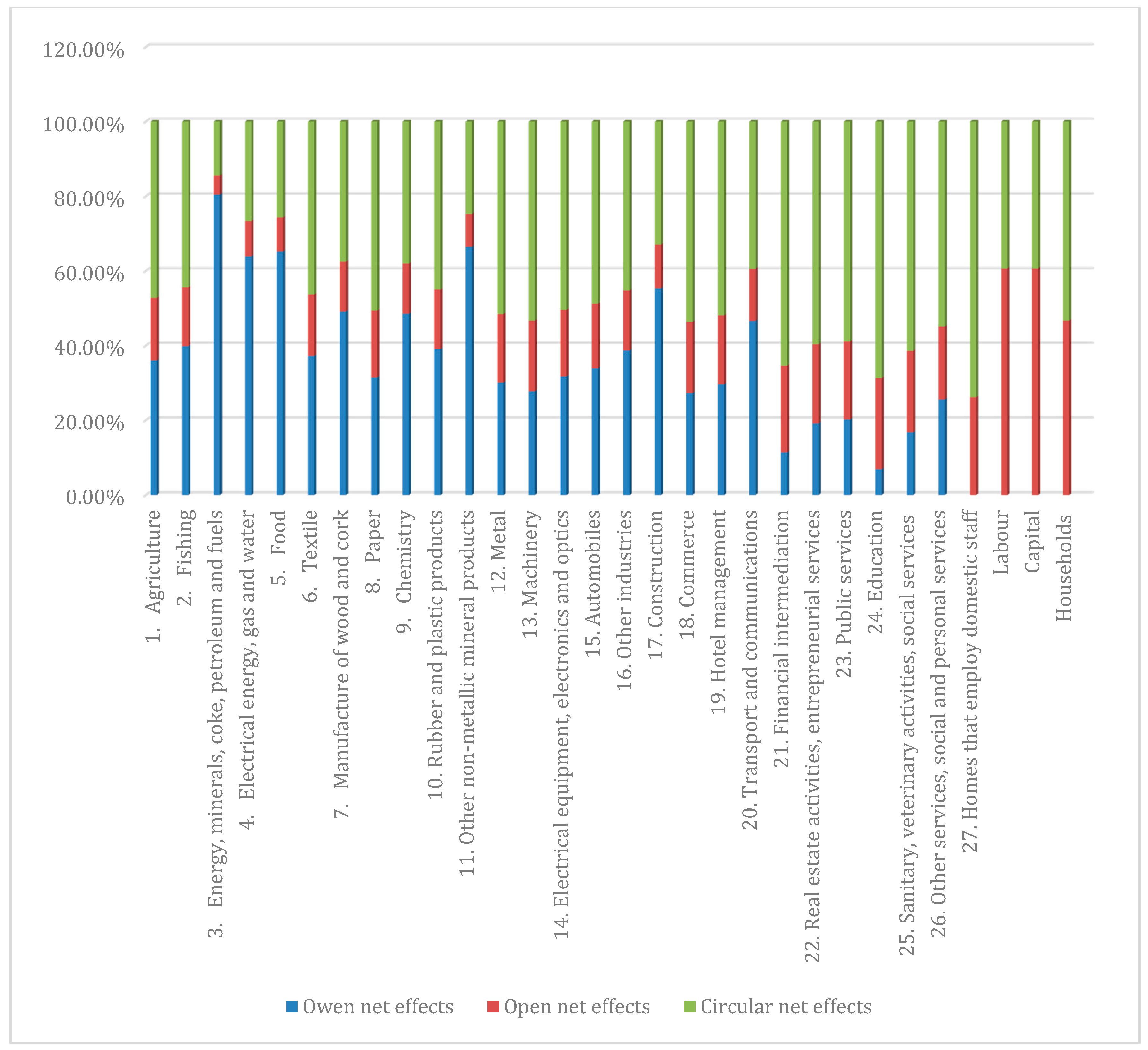
Figure 1 shows the results of the additive decomposition of the income multipliers, the NAMEA multiplier matrix of polluting emissions. In this paper, only the three emissions that show greenhouse gas pollution in the regional economy are used: methane (CH₄), carbon dioxide (CO₂) and nitrogen monoxide (N₂O). The original units of these four emissions have been rescaled to express them all in the same units, which are carbon dioxide equivalents. The analysis consists of calculating the matrices of own net effects $B\left(M_1-I\right)$ and open net effects and, last, the $B\left(M_3-I\right)M_2{M}_1$ matrix shows total circular net effects.

This table also reflects the values and percentages that each net effect contributes to the total emissions multipliers. Analysis of the table shows that circular effects with 45.66% of the total net effect and own effects with 33.33% have more weight than open effects (21.01%). On the other hand, it is important to note that in three accounts (labour, capital and households), open effects are considerably greater than circular effects. In these accounts and in account 27 (households which employ domestic staff), however, there are no own effects, either because of the high interrelation between the productive sectors, or due to the structure of the NAMEA which has only one account for the consumption sector, creating a possible limitation when the interrelations between the private sector and the economy are shown. Additionally, the sectorial values suggest that the contributions of the various components are highly asymmetric in quantitative terms.

5. Conclusions

Environmental tendencies, which can now be observed, require energetic and immediate measures involving politicians, businesses and citizens. If no changes are made, world deforestation will continue to advance to critical levels and the average global temperature could rise by up to 6.4 °C by the end of the century. Rising sea levels will endanger low-lying islands and coastal areas.

For the purposes of this paper, a linear model of emissions multipliers has been considered for the Catalan economy (2001). This model is used because it allows for analysing how exogenous and unitary inflows to final demand of production activities affect greenhouse gas emissions. In other words, this model illustrates the effects caused by an increase in units of exogenous demand on greenhouse gas emissions. Linear SAM models are similar (in terms of formal structure) to Leontief’s [5] open input–output model, but with the notable difference that SAM models incorporate a higher degree of endogeneity.

The NAMEA for Catalonia for 2001 was used to carry out this analysis, allowing for the interrelations between the economy and society (between the branches of activity and the institutional sectors and between these and the environment) to be better observed.

With the aim of reducing emissions in the Catalan economy in both the sectors which are not covered in the ETS and those that are, three possible scenarios were explored. In the first scenario, a reduction of emissions of CO₂ eq. of 10% in sectors 1, 2, 20 and 27 and of 21% in the remaining sectors were applied while keeping endogenous income constant, which achieved a general reduction of emissions. This would be a good policy for the environment, but is not a likely scenario since keeping endogenous income steady is unlikely.

In the second scenario, a reduction of emissions of CO₂ eq. of 10% in sectors not covered in the ETS (Sectors 1, 2, 20 and 27) and a reduction of 21% in the remaining sectors were applied, while reducing endogenous income (production and factorial and private income) by 8.6%, which achieved a general increase of all greenhouse gas emissions. This would not be a good policy for the environment because greenhouse gases would not be reduced and therefore the objectives signed by the European Union in 2008 would not be achieved.

In the third scenario, a reduction of emissions of CO₂ eq. of 10% in certain sectors (Sectors 1, 2, 20 and 27) and a reduction of 21% in the remaining sectors were applied, while increasing endogenous income by 8.6%. In this case, greenhouse gas emissions (tonnes of CO₂ eq.) were reduced per unit of exogenous demand. Therefore, a reduction in the total emissions together with an increase in endogenous income accounts would have a positive effect on the environment, which would enable the Catalan economy to achieve the objectives signed by the European Union in 2008.

In the current circumstances, the third scenario would be ideal, but, to be able to carry this out, public administration and companies would have their work cut out to be able to apply the different economic and environmental policies needed to achieve these objectives.

We can observe how, in all three cases, if we can reduce emissions, those that do achieve the objectives are sectors 1, 3, 4, 11, 14, 21, 26 and 27. This is, in fact, because these are sectors where the policies are implemented to a greater degree and therefore are more significantly affected.

The results also show that increases in greenhouse gas emissions essentially depend on the account that receives the exogenous inflow in demand. Greenhouse gas emissions in Catalonia are affected very differently at the sectorial level and the effects of production activities, factors and consumption on air pollution are very heterogeneous.

On the other hand, the results show that the different scenarios described have different effects on greenhouse gases. Because the pollutant shows a different sectoral pattern, the gas emissions must be analysed and treated individually to meet the targets set.

To complete this analysis, a decomposition of CO₂ eq. emissions was performed on own effects, open effects and circular effects. This decomposition shows the different channels of income creation and their effects on greenhouse gas emissions in the Catalan economy. For all the gases considered, the circular effects are the most important components in total multipliers. These results suggest that the different channels by which income effects can be produced have different effects on greenhouse gas emissions.

Finally, policies aimed at reducing emissions may clash with objectives for the development of societies, as there is a close relationship between economic growth and the consumption of natural resources. A link needs to be established between economic behaviour and the consumption of resources to achieve a better development model for societies while at the same time minimising damage to the environment.

References

- European Environment Agency. Approximated EU Greenhouse Gas Inventory: Early Estimates for 2011; EEA Report; European Environment Agency: Copenhagen, Denmark, 2012. [Google Scholar]
- European Environment Agency. Greenhouse Gas Emission Trends and Projections in Europe 2012; EEA Report; European Environment Agency: Copenhagen, Denmark, 2013. [Google Scholar]
- WWF Spain. Greenhouse Gas Emissions in Spain 1990–2012; WWF Spain: Madrid, Spain, 2013. [Google Scholar]
- Council of the European Union. Council Adopts Climate-Energy Legislative Package; Council of the European Union: Brussels, Belgium, 2009. [Google Scholar]
- Leontief, W. Environmental Repercussions and the Economic Structure: An Input-Output Analysis. Rev. Econ. Stat. 1970, 52, 262–271. [Google Scholar] [CrossRef]
- Ahmad, Y.J.; El Sefeary, S.; Lutz, E. Environmental Accounting for Sustainable Development; A UNEP-World Bank Symposium; The World Bank: Washington, DC, USA, 1989. [Google Scholar]
- Lutz, E. Toward Improved Accounting for the Environment: An UNSTAT-World Bank Symposium; The World Bank: Washington, DC, USA, 1993. [Google Scholar]
- United Nations. Integrated Environmental and Economic Accounting 2003. In Handbook of National Accounting; United Nations: New York, NY, USA, 2003. [Google Scholar]
- Pié, L. Multisectorial Models Applied to the Environment: An Analysis for Catalonia. Ph.D. Thesis, Universitat Rovira i Virgili, Reus, Spain, 2010. [Google Scholar]
- Manresa, A.; Sancho, F. Energy Intensities and CO2 Emissions in Catalonia: A SAM Analysis. Int. J. Environ. Workplace Employ. 2004, 1, 91–106. [Google Scholar] [CrossRef]
- Rodríguez, C.; Llanes, G.; Cardenete, M.A. Economic and Environmental Efficiency Using a Social Accounting Matrix. Ecol. Econ. 2007, 60, 774–786. [Google Scholar]
- Flores, M.; Sánchez, J. SAMEA for Aragon: Economic and Environmental Analysis. In Proceedings of the Second Spanish Conference of Input-Output Analysis: “Growth, Demand and Natural Resources”, Zaragoza, Spain, 5–7 September 2017. [Google Scholar]
- Duarte, R.; Mainar-Causapé, A.J.; Sánchez Chóliz, J. Domestic GHG emissions and the responsibility of households in Spain: Looking for regional differences. Appl. Econ. 2017, 49, 5397–5411. [Google Scholar] [CrossRef]
- Pyatt, G.; Round, J. Accounting and Fixed Price Multipliers in a Social Accounting Framework. Econ. J. 1979, 89, 850–873. [Google Scholar] [CrossRef]
- Pyatt, G.; Round, J. Social Accounting Matrices: A Basis for Planning; World Bank Symposium; The World Bank: Washington, DC, USA, 1985. [Google Scholar]
- Stone, R. The Disaggregation of the Household Sector in the National Accounts. In Proceedings of the World Bank Conference on Social Accounting Methods in Development Planning, Cambridge, UK, 16–21 April 1978. [Google Scholar]
- Defourny, J.; Thorbecke, E. Structural Path Analysis and Multiplier Decomposition within a Social Accounting Matrix Framework. Econ. J. 1984, 94, 111–136. [Google Scholar] [CrossRef]
- IDESCAT (Statistical Institute of Catalonia). Taules Input-Output Per a Catalunya; Institut d’Estadística de Catalunya: Catalonia, Spain, 2001. [Google Scholar]
- INE (Instituto Nacional de Estadística). Metodología. Las Cuentas Satélite sobre Emisiones Atmosféricas; Instituto Nacional de Estadística: Madrid, Spain, 2006.
- Stone, R. Input-Output and National Accounts; Organisation for European Economic Co-operation: Paris, France, 1961. [Google Scholar]
- Stone, R.; Brown, A. A Computable Model of Economic Growth; Chapman and Hall: London, UK, 1962. [Google Scholar]
- Miller, R.E.; Blair, P.D. Input-Output Analysis: Foundations and Extensions; Prentice-Hall International: Upper Saddle River, NJ, USA, 2009. [Google Scholar]
- Alcántara, V. Comptabilitat Satèl·lit del Medi Ambient. 2003. Available online: https://www.idescat.cat/estad/csc (accessed on 15 July 2017).
Figure 1.
Additive decomposition. Source: Compiled by author. Carbon dioxide equivalents; percentage.