The Impact of Aircraft Noise on Housing Prices in Poznan


1
Department of Microeconomics, Poznan University of Economics and Business, Al. Niepodleglosci 10, 61-875 Poznan, Poland
2
Department of Organization and Management Theory, Poznan University of Economics and Business, Al. Niepodleglosci 10, 61-875 Poznan, Poland
3
Department of Construction Management and Real Estate, Vilnius Gediminas Technical University, Sauletekio al. 11, LT-10223 Vilnius, Lithuania
*
Author to whom correspondence should be addressed.
Sustainability 2017, 9(11), 2088; https://doi.org/10.3390/su9112088
Submission received: 27 October 2017
/
Revised: 7 November 2017
/
Accepted: 10 November 2017
/
Published: 13 November 2017
(This article belongs to the Special Issue Sustainability in Construction Engineering)
Abstract
:In the paper, we analyzed the impact of aircraft noise on housing prices. We used a dataset containing geo-coded transactions for 1328 apartments and 438 single-family houses in the years 2010 to 2015 in Poznan. In this research, the hedonic method was used in OLS (ordinary least squares), WLS (weighted least squares), SAR (spatial autoregressive model) and SEM (spatial error model) models. We found strong evidence that aircraft noise is negatively linked with housing prices, which is in line with previous studies in other parts of the world. In our research, we managed to distinguish the influence of aircraft noise on different types of housing. The noise depreciation index value we found in our study was 0.87% in the case of single-family houses, and 0.57% regarding apartments. One of the reasons for the difference in the level of impact of aircraft noise may be the fact that the buyers of apartments may be less sensitive to aircraft noise than the buyers of single-family houses.
1. Introduction
Noise coming from aviation and its supporting operations is a crucial issue at airports across the world. The aviation industry has come a long way in efficiency and sustainability thanks to improvements in operations and technology [1]. It must be stated that huge improvements in technology have been made, so the level of noise coming from a single airplane is much lower than a few decades ago. Sustainable development in different aspects [2], as well as of air transport through the reduction of aircraft noise pollution at airports is promoted by the EU Environmental Noise Directive [3] and the associated Balanced Approach Regulation [4].
In recent years, air transport has grown in significance. In the pre-accession of Poland to the European Union period, in the years 1989–2004, air transport was developing very slowly [5]. After accession, post-socialist countries eliminated the barriers to entering their aviation markets [6,7]. Moreover, market liberalization resulted in new EU member countries being penetrated by low-cost carriers, which introduced new routes to destinations mainly in Western Europe [8].
Apart from the undoubted benefits of the sustainable development of society, this form of transport also generates some broadly defined costs (social and economic). There is no doubt that an increase in the level of aircraft noise is and will be an increasingly serious problem for people living in the vicinity of airports (both large international airports and less important local ones). This is connected with the development of regional airports and the intensification of air traffic in their area, but, most importantly, with the growing number of international flights. Three factors influence noise burden: the number of flights, the level of noise emitted by each airplane, and the time of flight. Other factors that may have an impact include flight paths and procedures, the distribution of flights in flight paths, or the use of runways. The characteristic features of aircraft noise are the fact that it occurs instantly, quickly obtains its maximum level, and then rapidly decreases. Consequently, many inhabitants of the areas surrounding airports complain about the level of noise, although the results of aircraft noise measurements show that it does not contribute to permissible noise levels being exceeded significantly. Given the above, it seems necessary to examine the consequences of the vicinity of an airport.
An overview of the studies of the negative influence of aircraft noise allows us to distinguish its most important spheres [9]:
- Physical and mental health of people influenced by an airport (numerous studies show that exposure to aircraft noise destabilises one’s mental condition, causes anxiety, increases aggression and excitability, raises blood pressure, disturbs heart and breath rhythms, reduces brain efficiency, and is the cause of an increased number of heart attacks and coronary diseases, as well as contributing to hearing deficiency or loss and speech disorders [10];
- Work efficiency (noise sensitivity increases the probability of disturbances in the execution of tasks and reduces work efficiency);
- Learning at schools (recent research shows a relationship between noise and children’s ability to learn and absorb information) [13];
- Voice communication (both indoors and outdoors; this may involve interfering a conversation, watching television, or listening to the radio);
- Using park and leisure areas (research shows that users find noise a very important factor influencing the quality of rest) [14];
- Air traffic noise has the most negative effect on housing prices. Meanwhile, road and train noises have similar but smaller effects [15];
- The market value of residential properties (almost all studies confirm the negative impact of noise on the market value of properties located near the airport).
In the paper, the influence of aircraft noise on the last of the above spheres will be discussed. Real properties are a specific good, which is a result of their physical, economic, institutional–legal and environmental features. The specificity of the real estate market is determined by the unique attributes of a property [16]. Structural and locational attributes could have been considered by house buyers as a vital factor in property transactions [17]. Having examined these features, it is justifiable to say that the market value of a property is influenced not only by its direct characteristics (such as the size and shape of a plot, the age of a building, construction type, technical condition [18]), but also factors that involve its broadly defined surroundings [19]. Studies of the determinants of housing prices in developed markets often take into account environmental components [20,21,22,23,24]. These factors may be divided into two groups according to the kind of impact: positive influence (e.g., the vicinity of green areas, bodies of water) and negative influence (e.g., noise, air pollution) [21]. The indoor environment of each building depends on some criteria, like temperature, humidity, noise, etc. [25,26].
The remainder of this paper is structured as follows. The next section presents a review of the literature on the relationship between aircraft noise and real estate prices in the areas surrounding an airport assessment. Section three presents study area, data collection and variables, and the methodological background of the hedonic models applied. Section four presents and analyzes the results obtained. The last section presents concluding remarks.
2. Literature Review
The externalities resulting from airport operation, particularly aircraft noise, represent social costs, which may be identified as a change in the value of properties located in the area affected by airport activities. The most frequently used methods of noise cost estimation included are based on revealed preferences. Revealed preferences are consumer choices, and they are analyzed with the use of historical data on property sales. Of all the models based on revealed preferences, the hedonic price model is the most frequently used method for analyzing the influence of airport operation on the property market.
In order to determine the annoyance costs related to noise, noise depreciation indices (NDIs) are used. NDIs are defined as the percent increase in the loss of property market values caused by a unit increase in noise exposure and are identified with the use of hedonic price methods. By now, there are approximately 50 HP studies for airports in Canada and the US, and probably an equal number of non-North American airports [27]. The aircraft noise literature has been previously reviewed by Nelson [27], Schipper et al. [28], Bateman et al. [29] and Wadud [30]. A summary of these studies is presented in Table 1.
These NDI estimates indicate that housing prices react differently across countries. This variation may be the result of different noise metrics (Noise Exposure Forecast (NEF), Noise Number Index (NNI), Australian Noise Exposure Forecast (ANEF), day–night sound Level (Leq, Ldn)), or different airport scales or different urban spatial structure. Otherwise different functional forms of models (linear, log-linear) used also account for a considerable part of the variation in these NDI estimates [30]. Moreover, some researchers argue that NDI and wealth are positively correlated. Wadud [30] carried out meta-regression analysis and concluded that the NDI tends to be higher in developed countries. Figure 1 summarizes the NDI estimates through a frequency distribution based on 79 studies carried out form 1970 till 2016 all over the world.
Taking into account some recent studies, most of them were carried out in Europe (Table 2). There are a few new analyses regarding European case studies [31,32,33,34,35,36,37,38,39,40,41,42,43,44]. All of these European analyses of the relationship between aircraft noise and real estate prices in the areas surrounding an airport confirmed a negative influence of aircraft noise on the market value of properties. The NDI ranges from 0.5% to 1.7% per decibel. However, difficulties may arise when comparing the obtained results since different noise indicators, thresholds, types of property and sources of data were used in these studies.
3. Methods and Data
3.1. Study Area
Poznan is located in Central-Western Poland, in the central part of Wielkopolskie Province. It is the fifth largest city in Poland by population (541.6 thousand inhabitants) and the eight largest by size (262 sq km). There are two airports within the administrative borders of the city of Poznan: Poznan Lawica International Airport and Poznan Krzesiny military airport, part of NATO structures.
Henryk Wieniawski Poznan Lawica International Airport (code IATA: POZ, code ICAO: EPPO), an international airport and one of the oldest airports in Poland, is located seven kilometres west of the centre of Poznan. As of 2015, it was the seventh largest Polish airport regarding the number of passengers carried and the number of airport operations (see Figure 2). Two modern passenger terminals ensure the capacity of 1900 passengers arriving and 1100 passengers departing per hour. In the years 2011–2013, owing to European funds, Lawica Airport was extended, and now it has a complex of passenger terminals which can handle up to 3.5 m passengers yearly.
Henryk Wieniawski Poznan Lawica International Airport operates regular flight connections to more than 30 airports. In recent years, it has handled approximately 1.5 million passengers a year (in the years 2010–2016).
In the case of Krzesiny, the 31st Air Base, it is an air force base located in South-East Poznan. The 31st Air Base is an air force unit for military operations conducted as part of the national defence system and a NATO very high readiness joint task force. In 2001, it was modernised so that it could handle F–16 aircraft. The grounds of the base have a rectangular shape. In the years 2001–2002, it was thoroughly modernized. It was actually entirely re-built. Now, it can handle practically all aircraft that are operated.
In comparison to 2011, in 2013 the total number of operations fell by 20.6% (from 6481 to 5143), with the number of night operations on almost the same level as in 2011 (see Figure 3). Such a big drop in the number of air operations significantly contributes to the improvement of the acoustic climate in the vicinity of the Poznań-Krzesiny airport. At the military airport in Poznan, supersonic multirole fighter aircraft F-16 Block 52+ are presently used. The 31st Air Base has 32 such planes.
3.2. Data Collection and Variables
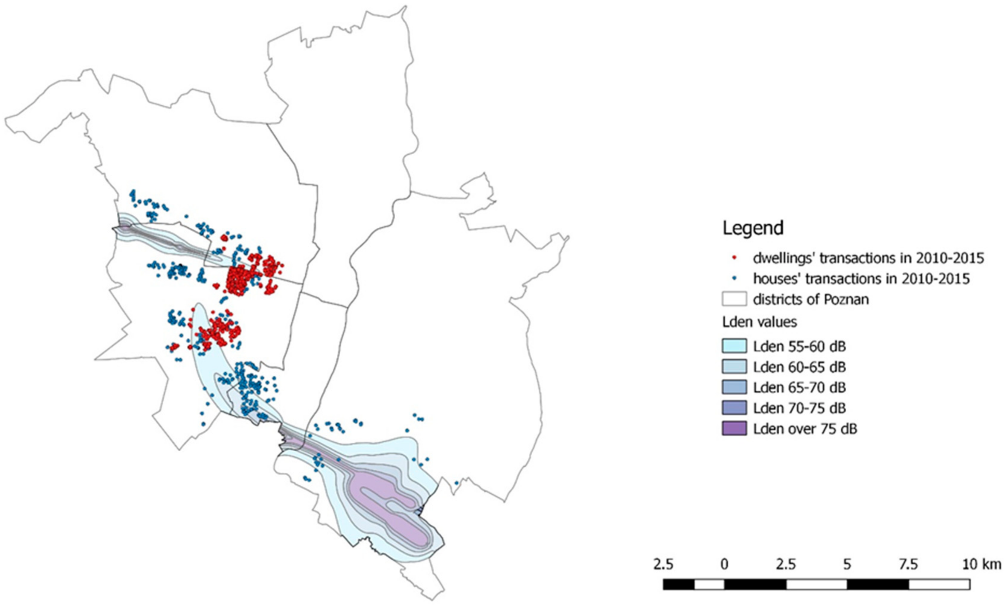
The research is based on transaction data (Figure 4 shows the map of Poznan, noise counters produced by two airports and property sales). The data on apartment transactions conducted from the first quarter of 2010 to the fourth quarter of 2015 was obtained from the Board of Geodesy and Municipal Cadastre in Poznan. The obtained data referred to the transactions concerning all kinds of properties, both residential and non-residential (e.g., commercial properties or garages). In the process of data cleansing, purchases of more than one residential unit and non-free market transactions (e.g., debt collector sales) were removed. The data included in notarial contracts concerning apartments contain the following information: the transaction date, the price, the area of an apartment, the floor on which an apartment is located, and the area of any auxiliary premises (e.g., a garage/parking spot in an indoor parking lot or a cellar/residents’ cupboard). Such a set of factors may bias the results of the research, as notarial contracts do not include information on strong pricing components such as, for example, the construction technology. Then, thanks to the cadastre data, a great deal of information on the height of buildings and the year of construction was added. Using the street view application on maps.google.com, the missing data concerning the height, year of construction, and, first of all, technology was provided. Then, with the use of Googlemaps API (application program interface), the addresses were geocoded (addresses of transactions).
The data included in notarial contracts concerning single-family houses contain the following information: the transaction date, the price, the area of plot, gross covered area. Then, thanks to the cadastre data, a great deal of information on the number of floors and the year of construction was added. Using the street view application on maps.google.com, the missing data concerning the number of overground and underground floors and the year of construction was provided. Moreover, we specified the type of roof (flat, sloping), the type of building (detached, semi-detached, terraced), the type of garage (whether an integral part of a house or detached), and, first of all, the technical condition of a building on the basis of external elements (based on historical photos). There is no doubt that floor space is an important factor regarding. Unfortunately, it is included in less than 10% of the observations in notarial deeds. That is why we decided to establish the area of a building taking into account the built-up area, number of aboveground floors, correction factor, the existence of a garage and the type of roof.
Spatial analyses were performed using the QGIS software. Those transactions, which took place within the area affected by aircraft noise (treatment group) and within 1.0 km from this zone (control group), were analyzed. In this research, apartments built before 1950 were excluded because such apartments are located mainly in the city center. Moreover, in the case of such apartments, the technical condition of a building is a significant determinant of their value (our dataset does not include this factor), which might affect the results obtained.
Table 3 and Table 4 summarize the descriptive statistics (mean and standard deviation) of the variables used in the study. Based on a distance of 1.0 km from the aircraft noise, we sorted the housing transactions into a treatment group consisting of properties located in the noise zone (single-family houses, 107 observations, and apartments, 158 observations) and a control group with properties located outside (1 km buffer, e.g., [45,46]) the aircraft noise zone (single-family houses, 331 observations, and apartments, 1170 observations). We used the transaction prices in the logarithm term as the response variable in our models.
The information on aircraft noise zones was taken from an acoustic map from 2012. Directive 2002/49/EC of the European Parliament requires the carrying out of a long-term policy of environmental protection against noise in the European Union countries. Its realization is based on the estimation of the long-term noise indicators Lden and Ln in the areas under protection. The threshold value used in this study was 55 dB. In order to establish both airports’ noise influence on the acoustic map of Poznań, the following data was used: the acoustic characteristics of the aircraft used, arrival and departure routes, glide paths, take-off and landing profiles, and the distribution of the intensity of flights during daytime, in the evenings and at night.
Within the reach of aircraft noise Lden (Lawica and Krzesiny airports combined), there were 2137 inhabitants in the range from 65 to 75 dB. The number of inhabitants exposed to Lden noise at a level of 55–65 dB is about 26,000.
3.3. Hedonic Price Models
Mathematical statistics methods are broadly applied to analyze the pricing of real estate [47,48,49,50,51,52,53,54]. The most commonly applied methods of housing evaluation are divided into two groups: traditional and advanced methods. The advanced methods include techniques such as hedonic price modelling (HPM), artificial neural networks (ANN), case-based reasoning, and spatial analysis methods. The HPM is an ideal analytical tool to analyze a non-homogeneous commodity regarding its attributes.
The first documented use of hedonic regression dates back to 1922, when G. A. Hass developed the farmland price model [55]. The first researcher to use the hedonic method to analyze the real estate market was probably Ridker, who aimed to identify the influence of pollution reduction on house prices [56]. The theoretical framework of the hedonic method was developed by Lancaster [57] and Rosen [58].
The idea of the hedonic method lies in the assumption that the price of heterogeneous goods may be characterised by their attributes. In other words, this method allows us to estimate the value of the particular attributes of a given product. The price of a given good is the response variable, while its quantitative and qualitative attributes are the explanatory variables. The equation may be written as follows (1):
where P is the price of a good, β is the regression coefficient, X is an attribute of a good (value driver), u is a random error.
One of the key issues in hedonic methods is the choice of the form of the regression function. The log-linear (natural logarithm) form of the regression function is most frequently used for studying changes in the real estate market in empirical research. As housing is a heterogeneous good, it is difficult to indicate a full list of crucial attributes. The heterogeneity of real estate hinders the measurement of price impacts. Taking into account Malpezzi [59] and Crompton’s [60] suggestions, six major categories of characteristics of housing may be distinguished: (1) structural attributes, (2) neighborhood related services and features, (3) location and accessibility, (4) environmental attributes, (5) community attributes and (6) time-related features. In our study, we examine the implicit value of the aircraft noise. We hypothesize that transaction price is a function of structural features, locational attributes, time and aircraft noise. The basic hedonic function of price (y) can be stated as:
In this research, we used several variants of hedonic regression, namely standard ordinary least squares (OLS), robust weighted least squares (WLS) and spatial models. According to WLS, the estimation was made with the following steps: an OLS regression was run, then the logs of the squares of residuals become the dependent variable in an auxiliary regression, on the right-hand side of which are the original independent variables plus their squares. The fitted values from the auxiliary regression were then used to construct a weighted series, and the original model was re-estimated using weighted least squares [61]. In recent years, a growing concern has risen regarding the spatial dependence found in most house price data. Spatial dependence intuition was presented by Tobler [62], who concluded that there is a reason to believe that things that are near will be more related than distant ones. As one of the most important features of the housing market is the importance of location, the hypothesis of the spatial dependence of house prices seems plausible. The spatial-lag model is based on the assumption that the spatially weighted average of housing prices in a neighbourhood affects the price of each house (indirect effects) in addition to the features of housing and neighbourhood characteristics (direct effects) [63]. The ordinary least squares (OLS) hedonic estimates are not biased, but estimation efficiency may be lowered by spatial dependence. The obtained results can be biased, especially regarding their statistical significance [64,65]. The model that deals with this interpretation of spatial dependence is called the spatial error model (SEM). In contrast, the spatial error model does not include indirect effects, but it assumes that there may be one or more omitted variable in the hedonic price equation and that the omitted variable(s) vary spatially [63]. Due to this spatial pattern in the omitted variables, the error term of the hedonic price equation tends to be spatially autocorrelated. The econometric model dealing with this kind of spatial dependence is called the spatial lag model, or spatial autoregressive (SAR) model. In the spatial lag model, spatial dependence is assumed to be present in the additional explanatory variable.
4. Results
Among the apartment characteristics checked for in the research were the following: year of transaction, area of the apartment, age, construction technology, floor, the height of the building, basement, distance to city center and finally range of aircraft noise. In the case of single-family houses, we used: year of the transaction, the area of the house, age of the building, underground floor, quality of the building, basement, garage, type of plot ownership, distance to city center and range of aircraft noise. The choice of qualitative and quantitative data was limited by the availability of information in the database. Table 5 presents the variables used in the study in case of single-family houses and Table 6 regarding apartments.
To address the research questions, hedonic regression equations using ordinary least squares and spatial models were estimated. The dependent variable was the natural log of a sales price. Gretl and Geodaspace software were used to estimate the parameters of functions.
Houses are heterogeneous in nature. This heterogeneity may be the reason for heteroscedasticity in the residuals of the estimation of the function. Indeed, we found heteroscedasticity in the case of apartments (there was no problem in case of single-family homes, according to Breusch–Pagan and Koenker–Basset tests). That is why we used OLS with heteroscedasticity correction (WLS). Moreover, we tested for the presence of multicollinearity as it leads to unstable coefficients and inflated standard errors. The variance inflation factors (VIFs) was used to detect multicollinearity. The VIF values in the model do not exceed 4.7 in case of single-family houses and 2.8 in case of apartments, which is in line with the most conservative rules of thumb that the mean of the VIFs should not be considerably higher than 10. Tests for the normality of residuals are presented in Table 7.
In order to test for the presence of spatial effects in the data, we calculated spatial weights between observations [66]. Based on the geographical coordinates, we created (438 × 438 for sing-family houses and 1328 × 1328 for apartments) spatial weight matrixes based on the distance between them; a 200 m for apartments and 400 m for single-family houses threshold distance d was assumed. We tested different threshold distances and decided to use these as they had the highest value of I-Moran statistics. Following the arguments of Anselin [67], tests for the presence of spatial effects were carried out (both spatial autocorrelation and spatial lag dependence). To conclude, we found strong evidence of spatial dependence in the form of spatial autocorrelation and spatial lag.
The estimation results for single-family houses are presented in Table 8 and for apartments in Table 9.
The estimated models were well-fitted in case of apartments, as they explained about 82% of the price variations. As far as for the single-family houses, the models explained from 65–66%, depending on the model. Almost all of the variables applied in the models turned out to be statistically relevant, and the expected coefficient signs were correct. The results of the spatial models (in the case of single-family houses and apartments) suggest that spatial effects were present in the data, in the form of unobserved variables and significant spatial processes (in the case of single-family houses).
We observed that within the period under study (2010–2015), time had a significant impact on transaction prices. It is worth mentioning that housing prices in the biggest cities in Poland increased by about 100% between 2006 and 2007 [68,69]. At the end of 2007, the subsequent decreasing phase in the property price cycle began, resulting from this abnormal price increase and the beginning of financial crisis [70]. It is worth noticing that in the case of single-family houses, this downturn was higher than considering apartments in the analyzed locations.
Taking into account the perspective of this paper’s objectives, the statistical relevance of the air-noise variable is important. The application of the log-linear model enabled the percentage difference in the price of the single-family house/apartment with similar characteristics located within aircraft noise zones and the 1.0 km buffer zone to be identified. The value of the air-noise coefficient in the SEM model (the regression coefficients obtained in models were similar, however for the interpretation we used the SEM model as it is most robust) reached the value of −0.0447 (Table 8), which indicates that a single-family house located in area affected by the aircraft noise was about 4.59% cheaper (in the area with aircraft noise level values of Lden 55–60 dB), 9.18% cheaper (in the area with aircraft noise level values of Lden 60–65 dB) and 13.77% cheaper (in the area with aircraft noise level values of Lden 65–70 dB) than a single-family house (with the same characteristics) located in the 1.0 km buffer zone (with aircraft noise under 55 dB) in the years 2010–2015. In case of apartments, this decrease was smaller- it was about 2.86% (Lden 55–60 dB).
5. Conclusions
To our best of our knowledge, this study is one of the first studies to address the effects of aircraft noise (measured with Lden) on real estate value in the post-socialist urban context. While the problem has been addressed in many articles, most of them focused on areas in the USA, Canada and Western European countries. Moreover, we managed to distinguish the influence of aircraft noise on different types of housing. In earlier studies, mainly one type of housing (for example apartments) was the basis of the analysis. It was difficult, actually impossible, to compare NDIs for different types of housing, taking into account differences in the location of airports, residential markets, various periods, measures of noise, model specifications.
This article aimed to identify the impact of aircraft noise created by airports on apartment and single-family house prices in Poznan. In this research, the hedonic method in OLS, WLS, SEM and SAR models were used. The application of the log-linear model allowed the identification of the percentage difference in the price of an apartment with similar features located within the noise zones and outside. In order to compare the obtained results with previous studies, we estimated the NDI values. The NDI value we found in our study was 0.87 in the case of single-family houses, which means there is a 0.87% value discount per decibel (Lden noise indicator). Regarding apartments, the NDI was a 0.57% decrease of value per 1 dB of aircraft noise. The reason for the difference in the level of impact of aircraft noise may be the fact that the buyers of such apartments may be less sensitive to aircraft noise than the owners of single-family houses, who, because of higher noise levels cannot fully take advantage of the benefits related to a single family home (e.g., limited enjoyment of their garden).
Our investigation showed that the sensitivity of buyers differs depending on housing type. Although the results are reasonable, our proposal is not without limitations, which are mainly related to the possible change of acoustic climates and the limitations of the dataset regarding the variables describing properties. Our study was made on based on the acoustic map from the year 2012, so some limitation may arise, as the acoustic climate of the city may have changed. However, we were not able to overcome this issue as the map is created every five years. On the other hand, taking into account the number of flights (a rather stable number), it may be assumed that aircraft noise did not change significantly. As far as the dataset is concerned, gathering the data for a housing market analysis is always a huge challenge. In the case of our research, we used different sources of information, however, we were not able to control directly for the quality of an apartment or a single-family house (inside). Moreover, the impact of aircraft noise in other cities in Poland may be different as the influence of wealth effects is regionally distributed.
In this regard, future research should be carried out in other cities in Poland so that it would be possible to compare NDI values from different airports. In order to increase the comparability of future research, they should be based on the same assumptions (variables describing the properties, time scope, methods used). It could provide a chance to examine the impact of regional wealth effects on NDI values.
Author Contributions
Radoslaw Trojanek and Justyna Tanas together designed the research and wrote the paper, Saulius Raslanas and Audrius Banaitis provided extensive advice throughout the study regarding the abstract, introduction, literature review, research methodology and data, and results of the manuscript. The discussion was a team task. All authors have read and approved the final manuscript.
Conflicts of Interest
The authors declare no conflict of interest.
References
- Hind, P. The Sustainability of UK Aviation: Trends in the Mitigation of Noise and Emissions; Independent Transport Commission: London, UK, 2016. [Google Scholar]
- Manzhynski, S.; Siniak, N.; Źróbek-Różańska, A.; Źróbek, S. Sustainability performance in the Baltic Sea Region. Land Use Policy 2016, 57, 489–498. [Google Scholar] [CrossRef]
- EC Directive 2002/49/EC of the European parliament and the Council of 25 June 2002 relating to the assessment and management of environmental noise. Off. J. Eur. Communities 2002, 189, 12–25. Available online: http://eur-lex.europa.eu/legal-content/EN/TXT/?uri=celex:32002L0049 (accessed on 27 October 2017).
- EC Regulation (EU). No 540/2014 of the European Parliament and of the Council of 16 April 2014 on the sound level of motor vehicles and of replacement silencing systems, and amending Directive 2007/46/EC and repealing Directive 70/157/EEC. Off. J. Eur. Communities 2014, 173, 65–78. [Google Scholar]
- Jankiewicz, J.; Huderek-Glapska, S. The air transport market in Central and Eastern Europe after a decade of liberalisation—Different paths of growth. J. Transp. Geogr. 2016, 50, 45–56. [Google Scholar] [CrossRef]
- Augustyniak, W. Efficiency change in regional airports during market liberalization. Econ. Sociol. 2014, 7, 85–93. [Google Scholar] [CrossRef] [PubMed]
- Olipra, Ł.; Augustyniak, W. Analysis of business traffic at Wroclaw Airport—Implications for economic development of the city and the region. J. Int. Stud. 2015, 8, 175–190. [Google Scholar] [CrossRef]
- Dobruszkes, F. New Europe, new low-cost air services. J. Transp. Geogr. 2009, 17, 423–432. [Google Scholar] [CrossRef]
- National Academies of Sciences, Engineering, and Medicine. Effects of Aircraft Noise: Research Update on Select Topics; Transportation Research Board: Washington, DC, USA, 2008; ISBN 978-0-309-09806-9. [Google Scholar]
- Swift, H. A Review of the Literature Related to Potential Health Effects of Aircraft Noise; Purdue University: West Lafayette, IN, USA, 2010. [Google Scholar]
- Basner, M.; Samel, A.; Isermann, U. Aircraft noise effects on sleep: Application of the results of a large polysomnographic field study. J. Acoust. Soc. Am. 2006, 119, 2772–2784. [Google Scholar] [CrossRef] [PubMed]
- Holt, J.B.; Zhang, X.; Sizov, N.; Croft, J.B. Airport noise and self-reported sleep insufficiency, United States, 2008 and 2009. Prev. Chronic Dis. 2015, 12, E49. [Google Scholar] [CrossRef] [PubMed]
- Clark, C.; Martin, R.; van Kempen, E.; Alfred, T.; Head, J.; Davies, H.W.; Haines, M.M.; Lopez Barrio, I.; Matheson, M.; Stansfeld, S.A. Exposure-Effect Relations between Aircraft and Road Traffic Noise Exposure at School and Reading Comprehension: The RANCH Project. Am. J. Epidemiol. 2005, 163, 27–37. [Google Scholar] [CrossRef] [PubMed] [Green Version]
- Rapoza, A.S.; Fleming, G.G.; Lee, C.S.Y.; Roof, C.J. Study of Visitor Response to Air Tour and Other Aircraft Noise in National Parks; Volpe National Transportation Systems Center: Cambridge, MA, USA, 2005. [Google Scholar]
- Kopsch, F. The cost of aircraft noise? Does it differ from road noise? A meta-analysis. J. Air Transp. Manag. 2016, 57, 138–142. [Google Scholar] [CrossRef]
- Renigier-Bilozor, M.; Wisniewski, R.; Bilozor, A. Rating attributes toolkit for the residential property market. Int. J. Strateg. Prop. Manag. 2017, 21, 307–317. [Google Scholar] [CrossRef]
- Kam, K.J.; Chuah, S.Y.; Lim, T.S.; Ang, F.L. Modelling of property market: The structural and locational attributes towards Malaysian properties. Pac. Rim Prop. Res. J. 2016, 22, 203–216. [Google Scholar] [CrossRef]
- Raslanas, S. Research of market value of multistory housing in Vilnius. Technol. Econ. Dev. Econ. 2004, 10, 167–173. [Google Scholar] [CrossRef]
- Trojanek, R.; Gluszak, M. Spatial and time effect of subway on property prices. J. Hous. Built Environ. 2017, 1–26. [Google Scholar] [CrossRef]
- Kaklauskas, A.; Zavadskas, E.K.; Raslanas, S. Modelling of real estate sector: The case for Lithuania. Transform. Bus. Econ. 2009, 8, 101–120. [Google Scholar]
- Zavadskas, E.; Kaklauskas, A.; Maciunas, E.; Vainiunas, P.; Marsalka, A. Real estate’s market value and a pollution and health effects analysis decision support system. In Proceedings of the 4th International Conference on Cooperative Design, Visualization, and Engineering, Shanghai, China, 16–20 September 2007; p. 191. [Google Scholar]
- Raslanas, S.; Tupenaite, L. Peculiarities of private houses valuation by sales comparison approach. Technol. Econ. Dev. Econ. 2005, 11, 233–241. [Google Scholar] [CrossRef]
- Źróbek, S.; Trojanek, M.; Źróbek-Sokolnik, A.; Trojanek, R. The influence of environmental factors on property buyers’ choice of residential location in Poland. J. Int. Stud. 2015, 8, 164–174. [Google Scholar] [CrossRef]
- McCord, J.; McCord, M.; McCluskey, W.; Davis, P.T.; McIlhatton, D.; Haran, M. Effect of public green space on residential property values in Belfast metropolitan area. J. Financ. Manag. Prop. Constr. 2014, 19, 117–137. [Google Scholar] [CrossRef]
- Raslanas, S.; Kliukas, R.; Stasiukynas, A. Sustainability assessment for recreational buildings. Civ. Eng. Environ. Syst. 2016, 33, 286–312. [Google Scholar] [CrossRef]
- Le Boennec, R.; Salladarré, F. The impact of air pollution and noise on the real estate market. The case of the 2013 European Green Capital: Nantes, France. Ecol. Econ. 2017, 138, 82–89. [Google Scholar] [CrossRef]
- Nelson, J.P. Meta-Analysis of Airport Noise and Hedonic Property Values: Problems and Prospects. J. Transp. Econ. Policy 2004, 38, 1–28. [Google Scholar]
- Schipper, Y.; Nijkamp, P.; Rietveld, P. Why do aircraft noise value estimates differ? A meta-analysis. J. Air Transp. Manag. 1998, 4, 117–124. [Google Scholar] [CrossRef]
- Bateman, I.; Day, B.; Lake, I. The Effect of Road Traffic on Residential Property Values: A Literature Review and Hedonic Pricing Study. Available online: http://www.gov.scot/Publications/2001/07/9535/File-1 (accessed on 27 October 2017).
- Wadud, Z. Using meta-regression to determine Noise Depreciation Indices for Asian airports. Asian Geogr. 2013, 30, 127–141. [Google Scholar] [CrossRef]
- Nguy, A.; Sun, C.; Zheng, S. Airport noise and residential property values: Evidence from Beijing. In Proceedings of the 17th International Symposium on Advancement of Construction Management and Real Estate; Springer: Berlin/Heidelberg, Germany, 2014; Volume 1, pp. 473–481. [Google Scholar]
- Baranzini, A.; Ramirez, J.V. Paying for Quietness: The Impact of Noise on Geneva Rents. Urban Stud. 2005, 42, 633–646. [Google Scholar] [CrossRef]
- Salvi, M. Spatial Estimation of the Impact of Airport Noise on Residential Housing Prices. Swiss J. Econ. Stat. 2008, 144, 577–606. [Google Scholar] [CrossRef]
- Dekkers, J.E.C.; van der Straaten, J.W. Monetary valuation of aircraft noise: A hedonic analysis around Amsterdam airport. Ecol. Econ. 2009, 68, 2850–2858. [Google Scholar] [CrossRef]
- Brandt, S.; Maennig, W. Road noise exposure and residential property prices: Evidence from Hamburg. Transp. Res. Part D Transp. Environ. 2011, 16, 23–30. [Google Scholar] [CrossRef]
- Thanos, S.; Wardman, M.; Bristow, A.L. Valuing Aircraft Noise: Stated Choice Experiments Reflecting Inter-Temporal Noise Changes from Airport Relocation. Environ. Resour. Econ. 2011, 50, 559–583. [Google Scholar] [CrossRef] [Green Version]
- Püschel, R.; Evangelinos, C. Evaluating noise annoyance cost recovery at Düsseldorf International Airport. Transp. Res. Part D Transp. Environ. 2012, 17, 598–604. [Google Scholar] [CrossRef]
- Huderek-Glapska, S.; Trojanek, R. The impact of aircraft noise on house prices. Int. J. Acad. Res. Int. J. Acad. Res. Part B 2013, 5, 397–408. [Google Scholar] [CrossRef]
- Trojanek, R. The impact of aircraft noise on the value of dwellings—The case of Warsaw Chopin airport in Poland. J. Int. Stud. 2014, 7. [Google Scholar] [CrossRef] [PubMed]
- Winke, T. The impact of aircraft noise on apartment prices: A differences-in-differences hedonic approach for Frankfurt, Germany. J. Econ. Geogr. 2016, 101. [Google Scholar] [CrossRef]
- Chalermpong, S. Impact of airport noise on property values. Case of Suvarnabhumi International Airport, Bangkok, Thailand. Transp. Res. Rec. J. Transp. Res. Board 2010, 2177, 8–16. [Google Scholar] [CrossRef]
- Boes, S.; Nüesch, S. Quasi-experimental evidence on the effect of aircraft noise on apartment rents. J. Urban Econ. 2011, 69, 196–204. [Google Scholar] [CrossRef]
- Ahlfeldt, G.M.; Maennig, W. External productivity and utility effects of city airports. Reg. Stud. 2013, 47, 508–529. [Google Scholar] [CrossRef] [Green Version]
- Lavandier, C.; Sedoarisoa, N.; Desponds, D.; Dalmas, L. A new indicator to measure the noise impact around airports: The Real Estate Tolerance Level (RETL)—Case study around Charles de Gaulle Airport. Appl. Acoust. 2016, 110, 207–217. [Google Scholar] [CrossRef]
- Cohen, J.P.; Coughlin, C.C. Changing noise levels and housing prices near the Atlanta airport. Growth Chang. 2009, 40, 287–313. [Google Scholar] [CrossRef]
- Cohen, J.P.; Coughlin, C.C. Spatial hedonic models of airport noise, proximity, an housing prices. J. Reg. Sci. 2008, 48, 859–878. [Google Scholar] [CrossRef]
- Raslanas, S.; Tupenaite, L.; Steinbergas, T. Research on the prices of flats in the south east London and Vilnius. Int. J. Strateg. Prop. Manag. 2006, 10, 51–63. [Google Scholar] [CrossRef]
- Deaconu, A.; Lazar, D.; Buiga, A.; Fatacean, G. Marginal prices of improvements made to blocks of flats: Empirical evidence from Romania. Int. J. Strateg. Prop. Manag. 2016, 20, 156–171. [Google Scholar] [CrossRef]
- Taltavull de La Paz, P.; López, E.; Juárez, F. Ripple effect on housing prices. Evidence from tourist markets in Alicante, Spain. Int. J. Strateg. Prop. Manag. 2017, 21, 1–14. [Google Scholar] [CrossRef]
- Lee, C.-C.; Lee, C.-C.; Chiang, S.-H. Ripple effect and regional house prices dynamics in China. Int. J. Strateg. Prop. Manag. 2016, 20, 397–408. [Google Scholar] [CrossRef]
- Chen, J.-H.; Ong, C.F.; Zheng, L.; Hsu, S.-C. Forecasting spatial dynamics of the housing market using Support Vector Machine. Int. J. Strateg. Prop. Manag. 2017, 21, 273–283. [Google Scholar] [CrossRef]
- Yang, H.; Song, J.; Choi, M. Measuring the Externality Effects of Commercial Land Use on Residential Land Value: A Case Study of Seoul. Sustainability 2016, 8, 432. [Google Scholar] [CrossRef]
- Del Giudice, V.; De Paola, P.; Manganelli, B.; Forte, F. The monetary valuation of environmental externalities through the analysis of real estate prices. Sustainability 2017, 9, 229. [Google Scholar] [CrossRef]
- Jayantha, W.M.; Lau, J.M. Buyers’ property asset purchase decisions: An empirical study on the high-end residential property market in Hong Kong. Int. J. Strateg. Prop. Manag. 2016, 20, 1–16. [Google Scholar] [CrossRef]
- Colwell, P.F.; Dilmore, G. Who Was First? An Examination of an Early Hedonic Study. Land Econ. 1999, 75, 620–626. [Google Scholar] [CrossRef]
- Coulson, E. Monograph on Hedonic Estimation and Housing Markets; Penn State University: State College, PA, USA, 2008. [Google Scholar]
- Lancaster, K.J. A new approach to consumer theory. J. Political Econ. 1966, 74, 132. [Google Scholar] [CrossRef]
- Rosen, S. Hedonic Prices and Implicit Markets: Product Differentiation in Pure Competition. J. Political Econ. 1974, 82, 34–55. [Google Scholar] [CrossRef]
- Malpezzi, S. Hedonic Pricing Models: A Selective and Applied Review. In Housing Economics and Public Policy; Blackwell Science Ltd.: Oxford, UK, 2008; pp. 67–89. ISBN 9780470690680. [Google Scholar]
- Crompton, J.L. The impact of parks on property values: A review of the empirical evidence. J. Leis. Res. 2001, 33, 1–31. [Google Scholar] [CrossRef]
- Cottrell, A. Gretl Manual: Gnu Regression, Econometrics and Time-Series Library; Wake Forest University: Winston-Salem, NC, USA, 2005. [Google Scholar]
- Tobler, W.R. A Computer Movie Simulating Urban Growth in the Detroit Region. Econ. Geogr. 1970, 46, 234–240. [Google Scholar] [CrossRef]
- Kim, C.W.; Phipps, T.T.; Anselin, L. Measuring the benefits of air quality improvement: A spatial hedonic approach. J. Environ. Econ. Manag. 2003, 45, 24–39. [Google Scholar] [CrossRef]
- Anselin, L.; Rey, S. Properties of Tests for Spatial Dependence in Linear Regression Models. Geogr. Anal. 1991, 23, 112–131. [Google Scholar] [CrossRef]
- Anselin, L. GIS Research Infrastructure for Spatial Analysis of Real Estate Markets. J. Hous. Res. 1998, 9, 113–133. [Google Scholar] [CrossRef]
- Wilhelmsson, M. Spatial Models in Real Estate Economics. Hous. Theory Soc. 2002, 19, 92–101. [Google Scholar] [CrossRef]
- Anselin, L. Exploring Spatial Data with GeoDa: A Workbook. Geography 2005, 244. Available online: http://www.csiss.org/ (accessed on 2 October 2017).
- Trojanek, R. An analysis of changes in dwelling prices in the biggest cities of Poland in 2008–2012 conducted with the application of the hedonic method. Actual Probl. Econ. 2012, 7, 5–14. [Google Scholar]
- Trojanek, M.; Trojanek, R. Profitability of Investing in Residential Units: The Case of Real Estate Market in Poland in the Period from 1997 to 2011. Actual Probl. Econ. 2012, 2, 73–83. [Google Scholar]
- Trojanek, R. Dwelling’s price fluctuations and the business cycle. Econ. Sociol. 2010, 3. [Google Scholar] [CrossRef] [PubMed]
Figure 1.
Frequency distribution of NDIs (79 studies from 1970 to 2016). Source: based on Wadud [27] and own research.
Figure 1.
Frequency distribution of NDIs (79 studies from 1970 to 2016). Source: based on Wadud [27] and own research.
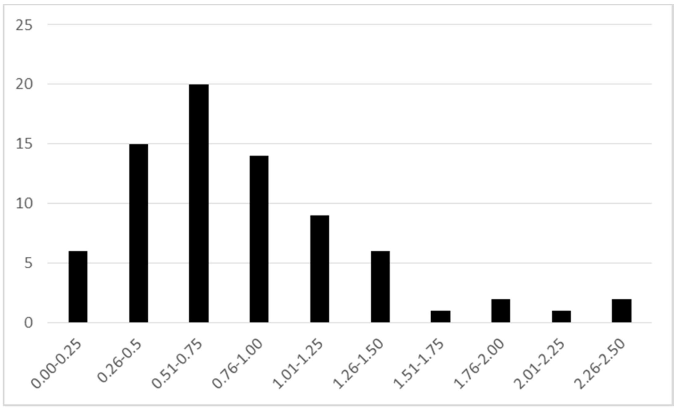
Figure 2.
Some passenger traffic and air operations at Lawica Airport. Source: Poznan Airport.
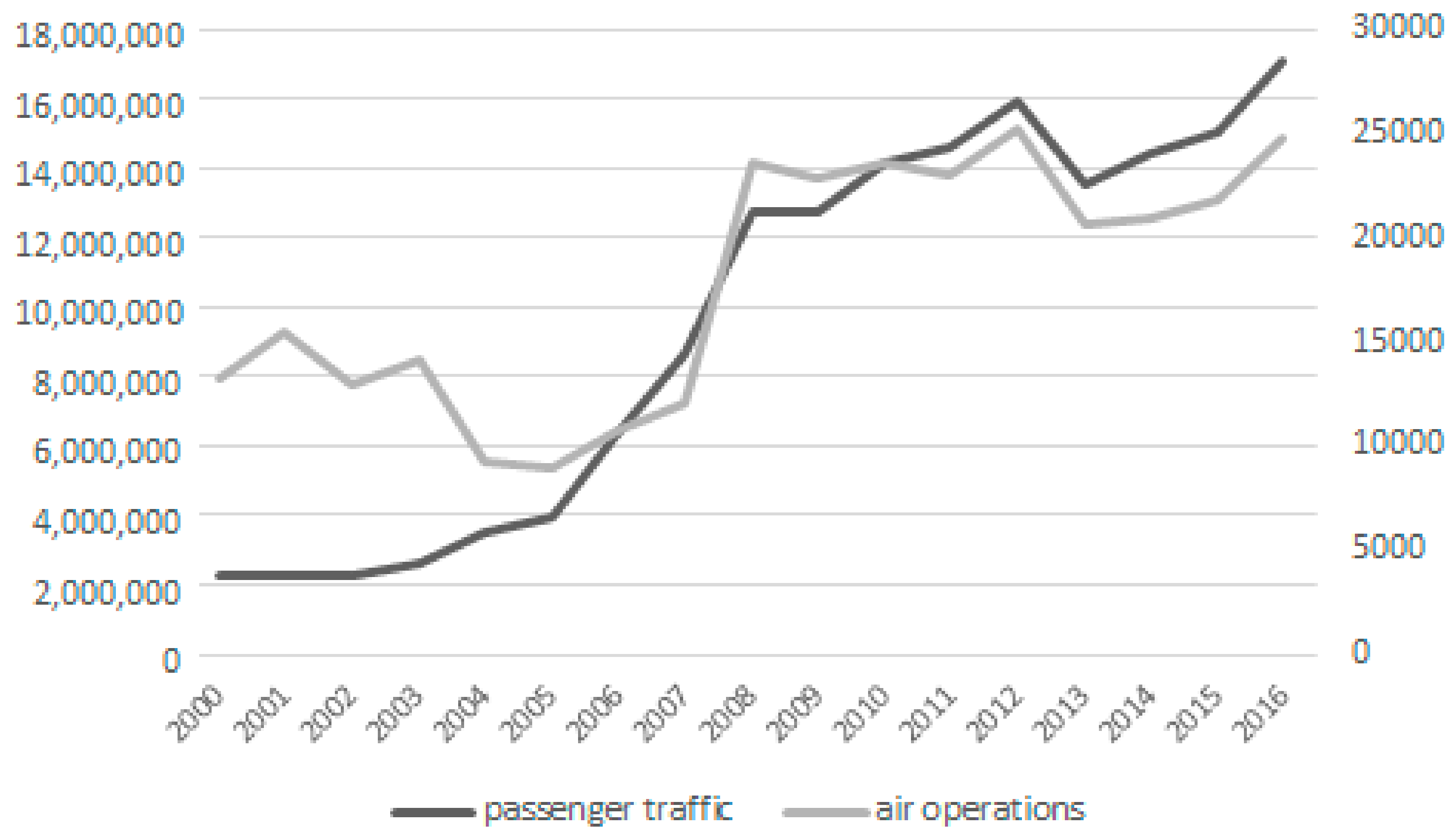
Figure 3.
A number of air operations at Krzesiny Military Airport. Source: Environmental protection program.
Figure 3.
A number of air operations at Krzesiny Military Airport. Source: Environmental protection program.
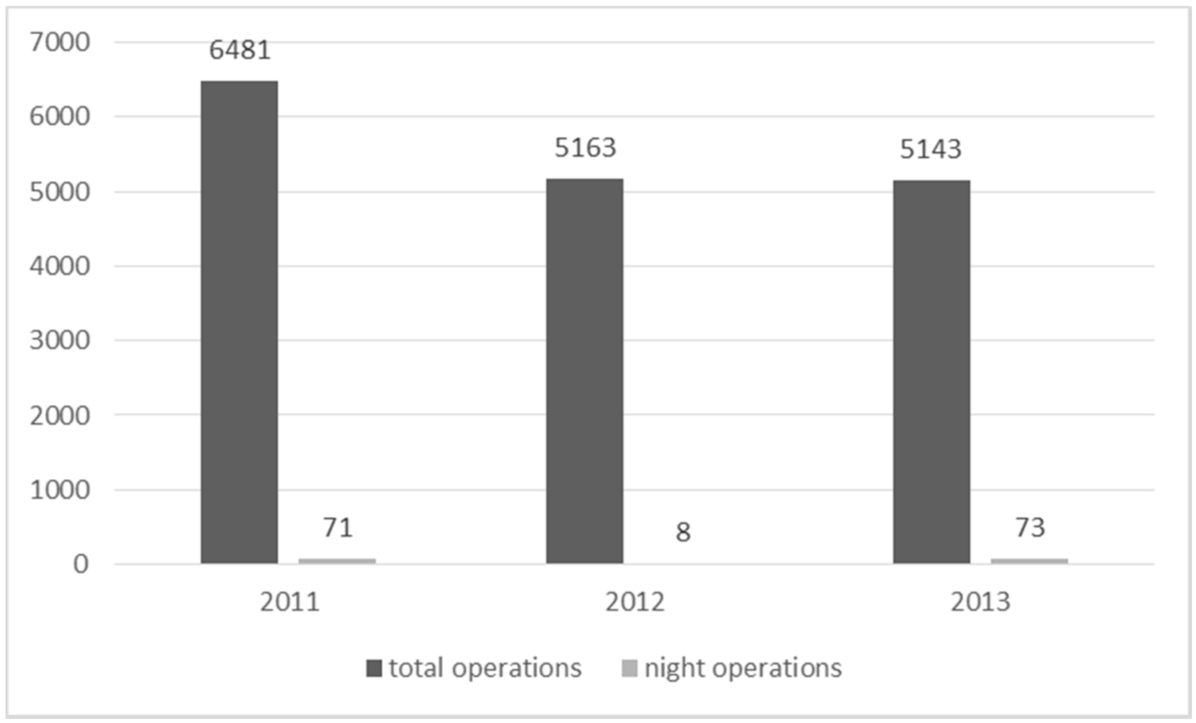
Figure 4.
Aircraft noise boundaries and property transactions included in the analysis. Source: Based on the Board of Geodesy and Municipal Cadastre in Poznan and own research.
Figure 4.
Aircraft noise boundaries and property transactions included in the analysis. Source: Based on the Board of Geodesy and Municipal Cadastre in Poznan and own research.


Table 1.
Summary of recent reviews of literature on aircraft NDIs (noise depreciation indices).
| Author(s) | NDI | Research Period | Study Area | Subject Scope |
|---|---|---|---|---|
| Nelson [27] | 0.28–1.49% | 1969–1993 | USA (17), Canada (6) | 23 airports, 33 NDI |
| Schipper et al. [28] | 0.1–3.57% | 1967–1996 | USA (21), Canada (5), Australia (2), UK (2) | 19 studies, 30 NDI |
| Bateman et al. [29] | 0.29–2.3% | 1960–1996 | USA (20), UK (5), Canada (3), Australia (2) | 30 studies |
| Wadud [30] | 0–2.3% | 1970–2007 | USA (35), Canada (8), Australia (8), the UK (8), the Netherlands (1), France (1), Switzerland (3) and Norway (1) | 65 studies |
Source: own research.
Table 2.
Summary of recent reviews of literature on aircraft NDIs.
| Id | Author(s) | Location | Noise Measure | Threshold dB | NDI | Research |
|---|---|---|---|---|---|---|
| 1 | Nguy et al. [31] | Beijing, China | – | – | 1.05% | 130 observations; sales; apartments; 2006–2012 |
| 2 | Baranzini and Ramirez [32] | Switzerland, Geneva | Ldn | 50 dB | 1.17% | 13,034 observations; rents; apartments; 2003 |
| 3 | Salvi [33] | Switzerland, Zurich | Leq16 | 50 dB | 0.97% | 3737 observations; sales; single-family houses; 1995–2005 |
| 4 | Dekkers and van der Straaten [34] | Netherlands, Amsterdam | Lden | 45 dB | 0.77% | 66,636 observations; sales; different types of properties; 1999–2003 |
| 5 | Brandt and Maenning [35] | Germany, Hamburg | Lden | 62 dB | 1.29% | 4832 observations; for sale; apartments; 2002–2008 |
| 6 | Thanos et al. [36] | Greece, Athens | Lden | 55 dB | 0.49% | 1613 observations; sales; different types of properties; 1995–2001 |
| 7 | Püschel and Evangelinos [37] | Germany, Düsseldorf | Lden | 55 dB | 1.04% | 1370 observations; for sale; apartments; November 2009 |
| 8 | Huderek-Glapska and Trojanek [38] | Poland, Warsaw | Laeq (The study is based on the Limited Use Area. The LUA is based on the actual noise indicators (LAeqD and LAeqN) around Warsaw airport and include the aircraft movements over the next five years.) | 55 dB | ~0.2% | 130324 observations; for sale; apartments; 2007–2011 |
| 9 | Trojanek [39] | Poland, Warsaw | Laeq Laeq (The study is based on the Limited Use Area. The LUA is based on the actual noise indicators (LAeqD and LAeqN) around Warsaw airport and include the aircraft movements over the next five years.) | 55 dB | ~0.8% | 5290 observations; sale; apartments; 2010 |
| 10 | Winke [40] | Germany, Frankfurt | Lden | 55 dB | 1.70% | 19148 observations; for sale; apartments; 2006–2014 |
| 11 | Chalermpong [41] | Thailand, Bangkok | NEF | 30 dB | 2.12% | 384 observations; sales; new homes; 2002–2008 |
| 12 | Boes and Nuesch [42] | Switzerland, Zurich | Leq16 | 30 dB–50 dB | 0.5% | 19,721 observations; for sale; rents; 2001–2006 |
| 13 | Ahlfeldt and Maenning [43] | Germany, Berlin | Lden | 45 dB | 0.5–0.6% | 31,289 observations; sales; different types of houses; 2000–2007 |
| 14 | Lavandier et al. [44] | France, Paris | Lden | 50 dB | Mean value 1.08% | 19,891 observations; sales; single-family houses; 2002–2008 (except 2007) |
| Mean value 1.51% | 23,264 observations; sales; apartments; 2002–2008 (except 2007) |
Source: own research.
Table 3.
Descriptive statistics of single-family house transactions.
| Control Group | Treatment Group | |||
|---|---|---|---|---|
| Mean | Standard Deviation | Mean | Standard Deviation | |
| y2010 | 0.10 | 0.30 | 0.16 | 0.37 |
| y2011 | 0.16 | 0.37 | 0.16 | 0.38 |
| y2012 | 0.17 | 0.37 | 0.14 | 0.35 |
| y2013 | 0.19 | 0.39 | 0.15 | 0.36 |
| y2014 | 0.17 | 0.38 | 0.20 | 0.40 |
| y2015 | 0.21 | 0.41 | 0.19 | 0.39 |
| Area | 157.08 | 52.71 | 155.86 | 58.55 |
| Transaction price (in PLN) | 579,935.68 | 212,738.75 | 540,635.91 | 213,968.57 |
| Age/10 | 2.72 | 1.72 | 2.98 | 1.63 |
| q1 | 0.11 | 0.31 | 0.10 | 0.31 |
| q2 | 0.15 | 0.36 | 0.20 | 0.40 |
| q3 | 0.29 | 0.45 | 0.35 | 0.48 |
| q4 | 0.24 | 0.43 | 0.22 | 0.42 |
| q5 | 0.21 | 0.41 | 0.13 | 0.34 |
| Underfloor | 0.45 | 0.50 | 0.50 | 0.50 |
| Garage | 0.76 | 0.43 | 0.78 | 0.42 |
| Areaplot | 453.19 | 253.80 | 443.53 | 270.23 |
| PU | 0.13 | 0.34 | 0.18 | 0.38 |
| Distance to CC | 6.12 | 1.31 | 6.16 | 0.70 |
| Airnoise5560 | 0 | 0 | 0.59 | 0.49 |
| Airnoise6065 | 0 | 0 | 0.24 | 0.43 |
| Airnoise6570 | 0 | 0 | 0.17 | 0.37 |
| No of observations | 331 | 107 | ||
Source: own research.
Table 4.
Descriptive statistics of apartment transactions.
| Control Group | Treatment Group | |||
|---|---|---|---|---|
| Mean | Standard Deviation | Mean | Standard Deviation | |
| y2010 | 0.18 | 0.38 | 0.11 | 0.31 |
| y2011 | 0.17 | 0.37 | 0.09 | 0.29 |
| y2012 | 0.15 | 0.36 | 0.16 | 0.37 |
| y2013 | 0.16 | 0.37 | 0.18 | 0.38 |
| y2014 | 0.18 | 0.39 | 0.18 | 0.38 |
| y2015 | 0.16 | 0.37 | 0.38 | 0.45 |
| Area | 44.34 | 13.26 | 48.41 | 13.47 |
| Transaction price (in PLN) | 226,411.72 | 75,402.95 | 241,305.46 | 72,835.37 |
| Age | 0.57 | 0.50 | 0.29 | 0.46 |
| Basement | 0.60 | 0.49 | 0.68 | 0.47 |
| Floor1 | 0.13 | 0.33 | 0.23 | 0.42 |
| Floor2 | 0.51 | 0.50 | 0.34 | 0.48 |
| Floor3 | 0.36 | 0.48 | 0.43 | 0.50 |
| Distance to CC | 4.32 | 1.03 | 5.24 | 0.90 |
| Airnoise5560 | 0 | 0 | 1 | 0 |
| Height2 | 0.31 | 0.46 | 0.22 | 0.42 |
| Technology2 | 0.52 | 0.50 | 0.55 | 0.50 |
| No of observations | 1170 | 158 | ||
Source: own research.
Table 5.
Qualitative and quantitative variables applied in the models in case of single-family houses.
Table 5.
Qualitative and quantitative variables applied in the models in case of single-family houses.
| Variable | Symbol | Description |
|---|---|---|
| Price | Price | Price for property (in PLN) |
| Year | y2010, y2011, y2012, y2013, y2014, y2015 | 6 time dummy variables used in the global model. If the apartment was sold in a given year, it takes the value 1; otherwise it takes 0 |
| Area | Area | Area of building = built-up area x number of overground floors (type of roof taken into account) × 0.8–20 m2 (if there is a garage in the building) |
| Age | Age | Age of the building divided by 10 |
| Quality | q1—new building to finish q2—the building is in bad condition q3—the building is in average condition q4—the building is in good condition q5—the building is in very good condition | 5 dummy variables. If the apartment is located on a given floor, it takes the value 1; otherwise it takes 0 |
| Underground floor | Underfloor | If there is underground floor than 1, if not 0 |
| Garage | Garage | If there is garage than 1, if not then 0 |
| Area of plot | Plotarea | Area of plot |
| PU | PU | 0—ownership of the plot 1—perpetual usufruct |
| Dcc | Dcc | Distance to city centre |
| Airnoise | Airnoise | 1—Lden 55–60 dB 2—Lden 60–65 dB 3—Lden 65–70 dB |
Source: own elaboration.
Table 6.
Qualitative and quantitative variables applied in the models in case of apartments.
| Variable | Symbol | Description |
|---|---|---|
| Price | Price | Price of an apartment (in PLN) |
| Year | y2010, y2011, y2012, y2013, y2014, y2015 | 6 time dummy variables used in the global model. If the apartment was sold in a given year, it takes the value 1; otherwise it takes 0 |
| Area | Area | Area of apartment m2 |
| Construction technology | Technology1—if the apartment is located in a building made with a prefabricated technology Technology2—if the apartment is located in a building made with a traditional technology | 2 dummy variables. If the apartment is located in a building made with given technology, it takes the value 1; otherwise it takes 0 |
| Age | Age | Age of the building |
| Floor | Floor1—ground and top floor Floor2—intermediate floors Floor3—first and second floor | 3 dummy variables. If the apartment is located on a given floor, it takes the value 1; otherwise it takes 0 |
| Height | Height1—buildings up to 4 floors Height2—buildings above 5 floors | 2 dummy variables. If the building has given height it takes the value 1; otherwise it takes 0 |
| Airnoise | Airnoise | If an apartment is located in aircraft noises in the range of 55–60 dB (Lden) then it takes value 1, otherwise it takes 0 (value under 55 dB) |
| Dcc | Dcc | Distance to city center in km |
| Basement | Basement | If an apartment has a basement then it takes value 1, otherwise it takes 0 |
Source: own elaboration.
Table 7.
Test for normality of residuals (Ordinary Least Squares models).
| Name of the Test | Single-Family Houses | Apartments |
|---|---|---|
| Doornik-Hansen | 2.34913, with p-value 0.308954 | 3.33477, with p-value 0.18874 |
| Shapiro-Wilk W | 0.995164, with p-value 0.189877 | 0.997589, with p-value 0.0494359 |
| Lilliefors | 0.0234289, with p-value ~= 0.81 | 0.0314622, with p-value ~= 0 |
| Jarque-Bera | 2.6041, with p-value 0.271974 | 3.27364, with p-value 0.194597 |
Source: own elaboration.
Table 8.
Estimation results (dependent variable is a natural logarithm of single-family house sale price).
Table 8.
Estimation results (dependent variable is a natural logarithm of single-family house sale price).
| OLS | WLS | SAR | SEM | |||||
|---|---|---|---|---|---|---|---|---|
| Variable | Coefficient | Probability | Coefficient | Probability | Coefficient | Probability | Coefficient | Probability |
| Constant | 13.5745 | 0.0000 | 13.5696 | 0.0000 | 13.2867 | 0.0000 | 13.6318 | 0.0000 |
| y2011 | −0.1062 | 0.0029 | −0.0968 | 0.0069 | −0.1024 | 0.0028 | −0.1110 | 0.0006 |
| y2012 | −0.1817 | 0.0000 | −0.1736 | 0.0000 | −0.1788 | 0.0000 | −0.1768 | 0.0000 |
| y2013 | −0.2629 | 0.0000 | −0.2487 | 0.0000 | −0.2604 | 0.0000 | −0.2817 | 0.0000 |
| y2014 | −0.2672 | 0.0000 | −0.2514 | 0.0000 | −0.2647 | 0.0000 | −0.2742 | 0.0000 |
| y2015 | −0.3336 | 0.0000 | −0.3247 | 0.0000 | −0.3300 | 0.0000 | −0.3334 | 0.0000 |
| Age | −0.0148 | 0.0626 | −0.0128 | 0.0750 | −0.0145 | 0.0589 | −0.0205 | 0.0085 |
| Area | 0.0020 | 0.0000 | 0.0021 | 0.0000 | 0.0020 | 0.0000 | 0.0018 | 0.0000 |
| Areaplot | 0.0001 | 0.0001 | 0.0002 | 0.0001 | 0.0002 | 0.0000 | 0.0002 | 0.0000 |
| Underfloor | 0.0865 | 0.0001 | 0.0774 | 0.0002 | 0.0882 | 0.0000 | 0.0726 | 0.0003 |
| Garage | 0.0443 | 0.0502 | 0.0552 | 0.0171 | 0.0448 | 0.0396 | 0.0374 | 0.0751 |
| q2 | −0.3008 | 0.0000 | −0.3398 | 0.0000 | −0.3024 | 0.0000 | −0.2626 | 0.0000 |
| q3 | −0.2049 | 0.0000 | −0.2337 | 0.0000 | −0.2060 | 0.0000 | −0.1696 | 0.0000 |
| q4 | −0.1024 | 0.0115 | −0.1498 | 0.0002 | −0.1044 | 0.0074 | −0.0685 | 0.0816 |
| q5 | 0.1078 | 0.0068 | 0.0561 | 0.1528 | 0.1008 | 0.0085 | 0.1272 | 0.0008 |
| PU | −0.0478 | 0.0806 | −0.0565 | 0.0216 | −0.0479 | 0.0692 | −0.0499 | 0.0552 |
| dcc | −0.0720 | 0.0000 | −0.0729 | 0.0000 | −0.0675 | 0.0000 | −0.0001 | 0.0000 |
| Airnoise | −0.0458 | 0.0001 | −0.0417 | 0.0001 | −0.0440 | 0.0001 | −0.0447 | 0.0061 |
| W_lnprice | 0.0188 | 0.0039 | ||||||
| Lambda | 0.40073 | 0.0000 | ||||||
| R-squared | 0.6582 | 0.6617 | ||||||
| Pseudo R-squared | 0.6675 | 0.6565 | ||||||
| N | 438 | 438 | 438 | 438 | ||||
Source: own elaboration.
Table 9.
Estimation results (dependent variable is a natural logarithm of apartment sale price).
| OLS | WLS | SAR | SEM | |||||
|---|---|---|---|---|---|---|---|---|
| Variable | Coefficient | Probability | Coefficient | Probability | Coefficient | Probability | Coefficient | Probability |
| Constant | 11.6100 | 0.0000 | 11.5313 | 0.0000 | 11.5641 | 0.0000 | 11.6653 | 0.0000 |
| y2011 | −0.0052 | 0.6653 | −0.0139 | 0.2697 | −0.0051 | 0.6710 | −0.0086 | 0.4505 |
| y2012 | −0.0577 | 0.0000 | −0.0576 | 0.0000 | −0.0576 | 0.0000 | −0.0595 | 0.0000 |
| y2013 | −0.0687 | 0.0000 | −0.0743 | 0.0000 | −0.0685 | 0.0000 | −0.0621 | 0.0000 |
| y2014 | −0.0273 | 0.0216 | −0.0328 | 0.0085 | −0.0271 | 0.0216 | −0.0291 | 0.0101 |
| y2015 | 0.0058 | 0.6291 | −0.0080 | 0.4847 | 0.0062 | 0.6009 | 0.0022 | 0.8489 |
| Dcc | −0.0334 | 0.0000 | −0.0338 | 0.0000 | −0.0333 | 0.0000 | −0.0387 | 0.0000 |
| Area | 0.0282 | 0.0000 | 0.0322 | 0.0000 | 0.0282 | 0.0000 | 0.0282 | 0.0000 |
| Area2 | −0.0001 | 0.0000 | −0.0002 | 0.0000 | −0.0001 | 0.0000 | −0.0001 | 0.0000 |
| Basement | 0.0288 | 0.0128 | 0.0262 | 0.0343 | 0.0284 | 0.0136 | 0.0136 | 0.2916 |
| Age | −0.0058 | 0.0000 | −0.0056 | 0.0000 | −0.0058 | 0.0000 | −0.0063 | 0.0000 |
| Floor2 | 0.0132 | 0.2382 | 0.0073 | 0.4731 | 0.0134 | 0.2267 | 0.0174 | 0.0972 |
| Floor3 | 0.0328 | 0.0028 | 0.0287 | 0.0045 | 0.0330 | 0.0024 | 0.0310 | 0.0024 |
| Height2 | −0.0402 | 0.0000 | −0.0378 | 0.0000 | −0.0398 | 0.0000 | −0.0279 | 0.0143 |
| Technology | 0.0495 | 0.0000 | 0.0463 | 0.0002 | 0.0493 | 0.0000 | 0.0313 | 0.0271 |
| Airnoise | −0.0252 | 0.0255 | −0.0263 | 0.0028 | −0.0251 | 0.0250 | −0.0290 | 0.0661 |
| W_lnprice | 0.0037 | 0.5140 | ||||||
| Lambda | 0.5739 | 0.0000 | ||||||
| R-squared | 0.8234 | 0.8221 | ||||||
| Pseudo R-squared | 0.8236 | 0.8213 | ||||||
| N | 1328 | 1328 | 1328 | 1328 | ||||
Source: own elaboration.
© 2017 by the authors. Licensee MDPI, Basel, Switzerland. This article is an open access article distributed under the terms and conditions of the Creative Commons Attribution (CC BY) license (http://creativecommons.org/licenses/by/4.0/).
Share and Cite
MDPI and ACS Style
Trojanek, R.; Tanas, J.; Raslanas, S.; Banaitis, A. The Impact of Aircraft Noise on Housing Prices in Poznan. Sustainability 2017, 9, 2088. https://doi.org/10.3390/su9112088
AMA Style
Trojanek R, Tanas J, Raslanas S, Banaitis A. The Impact of Aircraft Noise on Housing Prices in Poznan. Sustainability. 2017; 9(11):2088. https://doi.org/10.3390/su9112088
Chicago/Turabian StyleTrojanek, Radoslaw, Justyna Tanas, Saulius Raslanas, and Audrius Banaitis. 2017. "The Impact of Aircraft Noise on Housing Prices in Poznan" Sustainability 9, no. 11: 2088. https://doi.org/10.3390/su9112088
Note that from the first issue of 2016, this journal uses article numbers instead of page numbers. See further details here.