A Joint Optimal Decision on Shipment Size and Carbon Reduction under Direct Shipment and Peddling Distribution Strategies


1
School of Business, Ewha Womans University, Seoul 03760, Korea
2
College of Business Administration, Hongik University, Seoul 04066, Korea
*
Author to whom correspondence should be addressed.
Sustainability 2017, 9(11), 2061; https://doi.org/10.3390/su9112061
Submission received: 12 October 2017
/
Revised: 4 November 2017
/
Accepted: 6 November 2017
/
Published: 9 November 2017
(This article belongs to the Section Economic and Business Aspects of Sustainability)
Abstract
:Recently, much research has focused on lowering carbon emissions in logistics. This paper attempts to contribute to the literature on the joint shipment size and carbon reduction decisions by developing novel models for distribution systems under direct shipment and peddling distribution strategies. Unlike the literature that has simply investigated the effects of carbon costs on operational decisions, we address how to reduce carbon emissions and logistics costs by adjusting shipment size and making an optimal decision on carbon reduction investment. An optimal decision is made by analyzing the distribution cost including not only logistics and carbon trading costs but also the cost for adjusting carbon emission factors. No research has explicitly considered the two sources of carbon emissions, but we develop a model covering the difference in managing carbon emissions from transportation and storage. Structural analysis guides how to determine an optimal shipment size and emission factors in a closed form. Moreover, we analytically prove the possibility of reducing the distribution cost and carbon emissions at the same time. Numerical analysis follows validation of the results and demonstrates some interesting findings on carbon and distribution cost reduction.
1. Introduction
After the first deployment of the EU emission trading system (EU-ETS), emission trading systems to tackle climate change have spread across the world and covered 35 countries in 2015 by International Carbon Action Partnership(ICAP) [1]. Emission trading systems have effectively encouraged regulated polluters to make much effort towards managing and reducing carbon emissions. In line with the worldwide efforts to cut carbon emissions, business and industry have taken decarbonization into consideration in their logistics operations because a significant amount of carbon is emitted from freight transport and warehousing. According to World Economic Forum(WEF) [2], logistics contributes approximately 5.5% of the 50,000 megatons of carbon emissions generated by all human activity annually. Even more problematic is that the amount of carbon emitted by each tonne-km of freight movement also appears to be rising by Intergovernmental Panel on Climate Change(IPCC) [3], and freight traffic is predicted to grow at 2.3% annually from 2000 to 2050 in World Business Council for Sustainable Development(WBCSD) [4].
Lowering carbon emissions requires enormous changes in the operation of logistics, but shifting to low carbon logistics produces a concern about the classical models that have been widely used for designing and operating a logistics system. Although the traditional models have provided a solid theoretical foundation, we have doubts about whether the operational decisions (e.g., shipment size) developed based on the classical models are feasible when carbon costs are newly introduced.
Some research has recently addressed the question and extended the classical EOQ (Economic Order Quantity) model to include carbon emissions and its costs in developing an optimal decision. Hua et al. [5] and Chen et al. [6] used the classical framework of the EOQ model and analytically evaluated the impacts of carbon emissions on order decisions and costs. They also provided numerical results describing a condition under which carbon reduction is possible by modifying an order quantity. Bouchery et al. [7] proposed a multi-objective formulation of the EOQ model in which cost and carbon minimization constructs an efficient frontier and analytically find a Pareto optimum. Benjaafar et al. [8] considered a multi-period lot-sizing problem with a cap on carbon emissions and suggested the possibility of reducing carbon emissions by making an operational adjustment in an efficient manner. Bouchery et al. [9] extended the EOQ model into a two-echelon EOQ model and showed that coordination possibly enables lowering both cost and emissions. Konur [10] and Konur and Schaefer [11] integrated the EOQ model with transportation costs and considered different emission factors for various characteristics of a truck.
There is another direction of research incorporating carbon emissions into the classical Newsvendor model, which is effective in finding a single-period optimal production quantity under various carbon emission regulations; see [12,13,14]. Song and Leng [13] provided a basic idea on the use of the Newsvendor model and find an optimal production quantity with the consideration of carbon emissions. Zhang and Xu [14] extended the single-item Newsvendor model to the multi-item case and investigate the effects of carbon price and carbon cap on production quantity, profit, and carbon emissions.
Despite their wide use, there is a potential drawback in the literature based on the classical inventory models. According to Piecyk and McKinnon [15], carbon emissions are highly affected by the structure of a distribution system. For example, Ballot and Fontane [16] reveal that pooling inventory across locations reduces carbon emissions by increasing the chance to travel at full capacity and reducing travel distance. However, the classical inventory models fail to consider how the characteristics of distribution systems such as travel distance and customer density affect the amount of carbon emissions.
The joint decision on carbon reduction investment and operation is a new stream of research. An empirical study of Lai and Wong [17] suggests that improving productivity and operational performance is worth the costs of investment in implementation of green logistics management. In the context of a supply chain coordination, customer demand is formulated as a function of greening efforts that require upfront investment in [18,19]. They found a condition on the optimal greening effort to achieve better supply chain performance. Toptal et al. [20] extended the EOQ model to study joint decisions on order quantity and carbon reduction investment, and presented the possibility of reducing carbon emissions while reducing the cost. Similarly, Jiang and Klabjan [12] reformulated the Newsvendor model to study joint decision on production quantity and carbon reduction under carbon emission regulations. The current literature such as [12,18,19,20,21] has only dealt with the gross emissions in spite of the difference in technologies for managing carbon emissions from transportation and warehousing. Carbon emissions from energy use in the operation of logistics are broken down into two types: emissions from freight transport and emissions from storage by McKinnon [22]. While carbon emission in transportation is a function of travel distance and fuel efficiency, the inventory holding period and energy efficiency determine emissions at storage.
In this paper, we attempt to contribute to the literature on the joint decision on shipment size and carbon reduction by developing novel models for distribution systems under direct shipment and peddling distribution strategies. Unlike the literature that has simply investigated the effects of carbon costs on operational decisions, we address how to reduce carbon emissions and logistics costs by adjusting shipment size and making a decision on carbon reduction investment. Instead of using the framework of classical inventory models, we consider two different distribution systems so as to fully investigate the effects of the distribution structure (e.g., distribution strategy, travel distance, customer density, etc.) on carbon emissions and their costs. In particular, one of our research interests is coming up with a model covering the difference in managing carbon emissions from transportation and storage. To the best of our knowledge, no research has explicitly considered two sources of carbon emissions separately. This paper divides the gross emission into two components by separately determining emission factors (a.k.a. carbon intensity and emission intensity) from freight transportation and storage in the proposed model.
Based on our proposed models, the purpose of this paper is twofold. First, we find optimal shipment size and emission factors in order to minimize the total cost for delivering an item under direct shipment and peddling distribution strategies. The second is to show that a well-designed decision on shipment size and emission factors can reduce distribution costs as well as carbon emissions under direct shipment and peddling distribution strategies.
The rest of this paper is organized as follows. Section 2 begins with describing optimization models that formulate the cost for delivering items under direct shipment and peddling strategies. Section 3 and Section 4 present an optimal solution of both shipment size and emission factors for direct shipment and peddling strategy, respectively. Furthermore, we analytically show the possibility of carbon and cost reduction by adjusting shipment size and/or emission factors. In Section 6, we conduct numerical analysis to illustrate the results of our study. Section 7 concludes the paper with suggestions about a direction for future research.
2. Mathematical Model
Burns et al. [23] formulate the long-run average distribution cost for delivering an item from a depot (e.g., a manufacturing plant or a warehouse) to many customers under direct shipment and peddling distribution strategies. They find an optimal shipment size that minimizes the unit distribution cost including the transportation and inventory cost. We extend the model proposed by Burns et al. [23] to include the cost incurred by carbon emissions. The cost of carbon emissions considered in this paper is two-fold; the cost for trading carbon emissions under cap-and-trade regulation, which has been commonly considered in the literature, and the cost associated with the investment on carbon emissions.
The models are formulated with the notations that are summarized in Table 1. Throughout the paper, the superscript D and P represent direct shipment strategy and peddling strategy, respectively.
2.1. Modeling of the Direct Shipment Strategy
The direct shipment strategy allows each capacitated truck to visit only one customer in every delivery. The long-run average transportation cost per load is proportional to the total traveling distance and represented as . Customer demand is assumed to be known and arrive at a constant rate. We also assume that the production at the depot is perfectly coordinated with the customer demand. Under these assumptions, the average total time spent by a unit from production to consumption is given as (see Burns et al. [23]) and the long-run average inventory cost per unit becomes . Combining the transportation and inventory cost provides the unit logistics cost, , as similarly found in [23,24].
To formulate the cost for trading carbon emissions, we first propose the amount of carbon emission denoted by . Carbon emissions are mainly from energy consumed in transportation and storage. Let c and h denote carbon emission factors in transportation and warehousing, respectively (see WRI [25] for a detailed description on emission factors). A few papers in the literature formulated emission factors as a function of load factors or vehicle types [10,11,26]. For example, the emissions from an empty truck were defined independently from the emission from delivering items. In this paper, the emissions from an empty truck is assumed to be a part of the emission factor in warehousing because of their structural similarity as defined in [10,11]. For simplicity, an average load factor is assumed to be a part of the emission factors, which means we consider homogeneous trucks similar to [27]. Furthermore, the weight of a load is ignored when calculating the amount of carbon emission. For carbon emission factors c and h, we have that . For a given carbon cap K, we have to determine the amount of carbon trading x such that . If x is negative (i.e., ), then it costs to buy emission permits. On the contrary, a positive value of x adds profit into the model.
McKinnon et al. [28] emphasized the importance of improving energy efficiency and lowering carbon emission factors of energy used in transportation and warehousing operations. Lowering emission factors can be achieved by introducing low carbon technologies for vehicles (e.g., aerodynamic fairings, hybrid and electronic vehicles, replacing diesel with environmental friendly fuels, low-rolling resistance tires and anti-idling devices, etc.) and designing energy efficient warehouses (e.g., energy efficient lightning systems and material handling equipment, etc.). For example, FedEx operates hybrid-electric vehicles and LPG (Liquefied Petroleum Gas)-powered ground support equipment at its hub and other warehousing facilities across the world. FedEx reported that the hybrid trucks reduced carbon emissions by 30% in the U.S. [29]. For reference, low carbon technologies for logistics operations are presented in Dey et al. [30] and McKinnon [22].
These technology-driven efforts to improve emission factors should be accompanied by additional costs. Some literature argues that the cost is convex and increasing as lowering emission factors [18,19]. However, we use a linear cost function similar to Jiang and Klabjan [12], and convex cost functions are numerically evaluated in Section 6. The costs for lowering emission factors from their initial values and to c and h are given as . Keeping the initial values and incurs no cost, but it costs more by lowering c and h. The emission factors are assumed to be bounded below and not allowed to be less than and .
By combining theses cost components, we obtain the distribution cost denoted by for the direct shipment strategy (This section is based on our previous work in [31], and we redescribe the model to help readers easily understand further analysis.):
Let and so that F and H imply the transportation and inventory holding cost considering carbon emissions. Replacing x with yields the following simpler model:
2.2. Modeling of the Peddling Strategy
In each delivery, the peddling strategy allows a vehicle to visit several customers within a defined delivery region. Thus, the total travel distance includes not only the round trip distance L but also local delivery distance. Let n and m denote the number of customers within the delivery region and the number of customer stops per delivery, respectively. For given n and m, Stein [32] shows that the local delivery distance becomes , where is customer density and k is a constant of which its value is approximately 0.6. Readers are recommended to see Burns et al. [23] that provides detailed description on how to determine n and m.
In this paper, we consider a situation in which a vehicle should visit all customers within a delivery region in each delivery. This is generally found when the vehicle capacity is substantially larger than the demand in a delivery region and would likely fit the case where a depot delivers items via fixed routes. Based on this consideration, we can now assume that and provide closed form expressions for decision variables and analytical results. Finally, the long-run average transportation cost per unit for peddling strategy is given as , where .
The inventory holding cost for a peddling strategy is similar to that in a direct shipment model except for the customer demand. Unlike the direct shipment strategy, it needs to take account of several customers within a delivery region. When assuming all customers are identical, the total demand from n customers is . Thus, the long-run average inventory holding cost per unit becomes .
Combining carbon emissions in transportation and warehousing provides the amount of carbon emissions when emission factors are c and h. Then, the problem for peddling distribution strategy is formulated as follows:
Let which represents the unit transportation cost for local delivery and (i.e., ). Reorganizing the model by replacing x with provides the model for peddling distribution strategy:
3. Optimal Solutions
3.1. Direct Shipment Strategy
We first find an optimal point that minimizes based on our previous work in Min [31]. Because of the convexity of with respect to q, for given c and h, the optimal shipment size is determined as , where from the first order condition . Note that the optimal shipment size can be a full truck load. However, since it becomes too trivial when the vehicle travels with its full load (i.e., ), we only consider the case of less than a full truck load. Replacing q in Equation (1) with simplifies as follows:
Proposition 1.
is jointly concave in c and h.
Proof.
Let denote the Hessian of . Then,
is negative semidefinite because the first leading principal minors of are negative and . It concludes that is jointly concave in c and h. ☐
In addition to the concavity of in Proposition 1, the classical extreme value theorem specifies the existence of an optimal point that minimizes when c and h are bounded. Furthermore, the minimizer is on the boundary of c and h based on the concavity of . The following Proposition 2 describes how to determine the optimal values of c and h.
Proposition 2.
The optimal carbon emission factors are as follows:
where , , , , , , and
Proof.
The proof follows Theorem 1 in Min [31]. ☐
In Proposition 2, and represent the transportation cost when and , respectively. () represents the transportation cost reduction by lowering the carbon emission factor from to when (). Similarly, () is the reduction achieved in the inventory holding cost by adjusting the warehousing emission factor. In this sense, we observe that the optimal levels of emission factors are situational with respect to the unit cost for lowering carbon emission factors together with the expected cost reduction. For example, and that are larger than the anticipated cost reduction in transportation () and warehousing () lead to the decision of making no investment on lowering emission factors and keeping the initial values and .
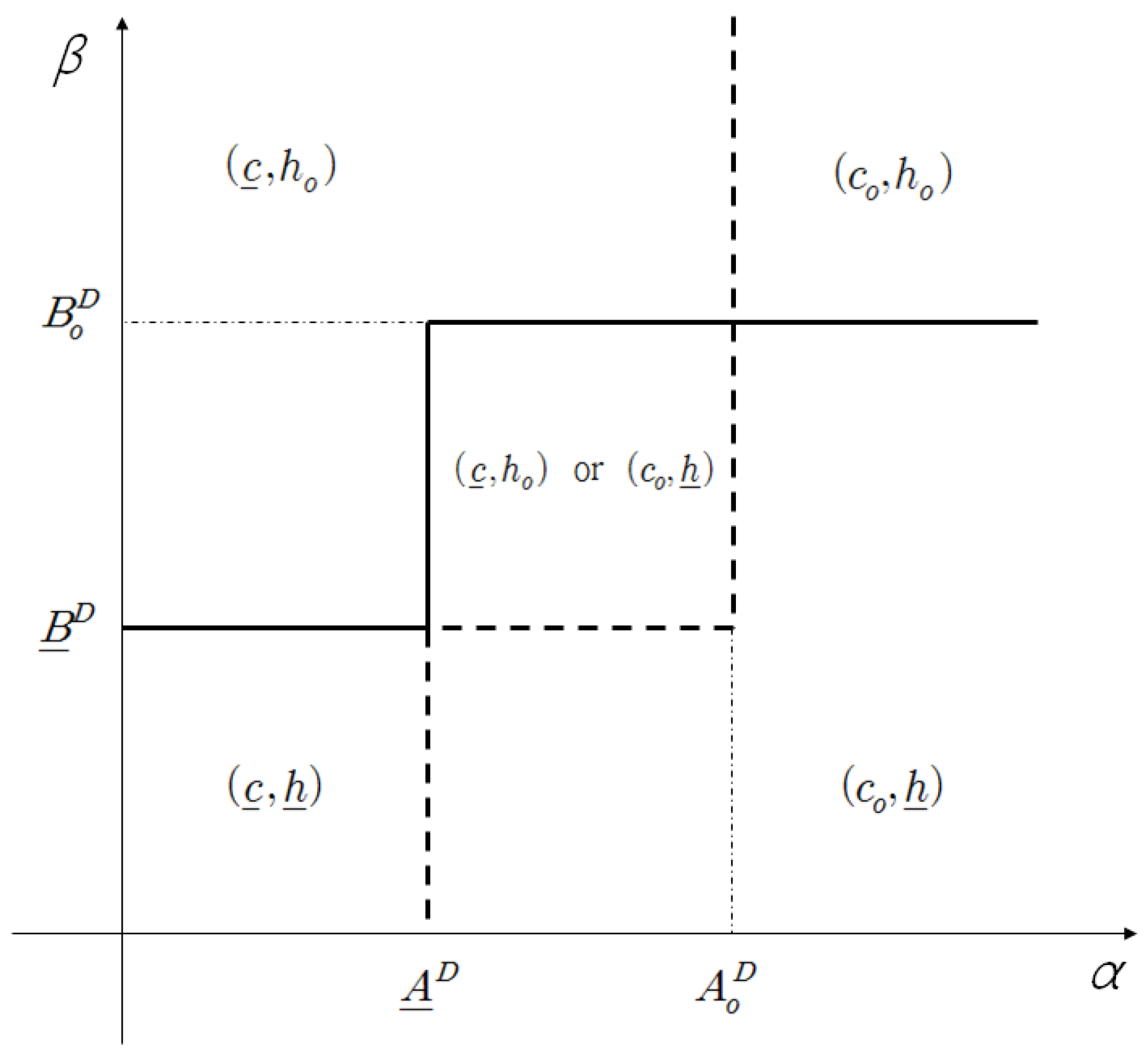
Figure 1 graphically illustrates Proposition 1 and shows that the policy for determining carbon emission factors is of the control limit-type. When falls below the dotted line representing the control limit for the emission factor in transportation, the carbon emission factor c is switched over to from .
It is noteworthy that determining the optimal values of c and h depend on each other when both and are at intermediate levels. If is larger than or smaller than , determining or is independent of . However, should be taken into account in determining whether to lower the emission factor c when is in between and . The inter-dependency of the decisions on c and h relies on the difference in cost reduction attained by lowering an emission factor over another. For example, too large a value of makes it hard to expect significant cost reduction by lowering carbon emissions at storage. Thus, if is at an intermediate level while is large, then it is more likely to achieve more cost reduction by lowering carbon emissions in transportation rather than at storage. In Figure 1, we observe is switched over to as increasing when is in between and .
3.2. Peddling Strategy
Similar to the procedure in Section 3.1, we find an optimal solution that minimizes the distribution cost under the peddling strategy . In the case of a direct shipment strategy, we observe that a vehicle could travel with less than a full truck load. However, for the peddling strategy, a truck should travel with its full capacity in each delivery so as to minimize the distribution cost.
Proposition 3.
An optimal shipment size is the vehicle capacity (i.e., ).
Proof.
Because a truck traveling with its full capacity is assumed to visit all customers in each delivery (i.e., ), there needs to be a determination of the number of visits that minimizes the distribution cost. From Equation (2), the derivative of with respect to n (i.e., ) provides an optimal number of visits with . After eliminating and , we can simplify Equation (2) into as follows:
Like the case of direct shipment strategy, the concavity of follows the finding of optimal emission factors that minimizes .
Proposition 4.
is jointly concave in c and h.
Proof.
Let denote the Hessian of . Then,
Because the first leading principal minors of are negative and , is negative semidefinite. This completes the proof. ☐
Proposition 5.
The optimal carbon emission factors are obtained as follows:
where , , , , , and
Proof.
We consider the following four cases.
- (1)
- ,Since is concave in c, the minimum point is determined at or ..
- (2)
- ,.
- (3)
- ,.
- (4)
- ,.
☐
4. Reducing Carbon Emissions and Distribution Cost
4.1. Direct Shipment Strategy
This section investigates whether it is possible to reduce carbon emissions as well as the distribution cost by adjusting shipment size and carbon emission factors to the optimal values as found in Proposition 2. Recall that the optimal shipment size is , where and are the transportation and inventory holding costs with the optimal emission factors and . Let denote an optimal shipment size when and . Then, . We now show that the following Theorem 1 on carbon emissions holds.
Theorem 1.
. It means that adjusting the shipment size and emission factors to their optimal levels (, and ) reduces carbon emissions.
Proof.
and let .
- (i)
- If , then
- (ii)
- If , then and .and by the definitions of and . Thus, .
- (iii)
- If , then and .and by the definitions of and . Thus, .
- (iv)
- If , then and .
- (a)
- If , then .
- (b)
- If , then it needs to show ..Because , we conclude and .
- (c)
- When , it can be similarly shown that .
From (i)–(iv), we conclude . ☐
From Theorem 1, we see that reducing emission factors leads to an emission reduction. Now, we investigate the effect of including cost associated with carbon emissions in determining the shipment size on the reduction in carbon emissions. In particular, we show that adjusting the shipment size, when considering the carbon costs lowers the carbon emissions. Let denote an optimal shipment size when ignoring carbon costs, and . That is, the inequality holds as shown in the following Theorem 2.
Theorem 2.
Carbon reduction is possible by including the cost associated with carbon emissions in determining the shipment size if .
Proof.
and .
- (i)
- If (i.e., ), then there is no difference between and .
- (ii)
- If (i.e., ), then it is easy to show by applying and into the inequality. Thus, .
- (iii)
- Similarly, (i.e., ) leads to and .
From (i)–(iii), it concludes the proof. ☐
We have a similar analytical result in Theorem 2 with the finding proposed by Chen et al. [6]. By using the EOQ framework, Chen et al. [6] argue that modifying order quantities possibly reduces carbon emissions only if , where A and h are ordering and inventory holding cost and and are emissions associated with placing an order and holding an item in inventory, respectively. In the case of , carbon emissions are at their minimum regardless of how to adjust the shipment size considering carbon costs.
Corollary 1.
A carbon emission reduction is possible by adjusting the shipment size and emission factors considering carbon costs if .
Proof.
From the previous two theorems, we conclude that . ☐
Corollary 1 indicates the possibility of carbon emission reductions by adjusting the shipment size or emission factors. Now, we investigate cost reduction.
Theorem 3.
Reducing the distribution cost is possible by adjusting the shipment size and emission factors if .
Proof.
We prove .
and
.
- (i)
- If , thenif and if .
- (ii)
- If , thenwhere the inequality holds because .According to the result of (i), we conclude .
- (iii)
- If , thenwhere the inequality holds because .According to the result of (i), we conclude .
- (iv)
- If , thenwhere the inequality holds because and .
From (i)–(iv), we conclude if . ☐
In addition to an emission reduction, Theorem 3 shows that cost reduction can be achieved by adjusting the shipment size or the emission factors. Because we determine an emission factor at which it minimizes the distribution cost by evaluating the trade-off between the cost for lowering the emission factor and the gains from an operational cost reduction, it is easy to understand why a distribution cost reduction is possible. However, even if we make no change in the emission factors from their initial levels and , cost reduction is attainable by modifying the shipment size if . An interesting finding is that is the only condition required for simultaneously reducing both carbon emission and distribution cost.
4.2. Peddling Strategy
We analytically investigate the possibility of carbon and cost reduction under the peddling strategy by using the amount of carbon emissions given as . As shown in Proposition 3, the distribution cost is minimized when the shipment size is U. Thus, unlike the case of the direct shipment strategy, adjusting shipment size is not a significant means of reducing carbon emissions and cost. Thus, we mainly consider the effects of adjusting emission factors to their optimal levels on carbon emissions and distribution cost.
Theorem 4.
Adjusting emission factors reduces carbon emissions.
Proof.
We need to show .
- (i)
- If , then
- (ii)
- If , then .Since , it is trivial to show the inequality holds. Thus, because and .
- (iii)
- If , then .When considering , it is easy to show . Thus, because .
- (iv)
- If , then .
Applying and yields and , and it supports .
From (i)–(iv), we conclude . ☐
Corollary 2.
Adjusting emission factors reduces the distribution cost.
Proof.
We need to show , but the proof is trivial because is the point that minimizes . An explicit proof is also shown below.
- (i)
- If , then
- (ii)
- If , then .Because when , .
- (iii)
- If , then .Because when , .
- (iv)
- If , then .Because and , .
The conclusion from (i)–(iv) completes the proof of . ☐
There is no required condition to satisfy for reducing emissions and cost. The condition that is found under the direct shipment strategy is mainly due to the shipment size, but no modification is allowed under the peddling strategy. Thus, we observe that lowering at least one of carbon emission factors leads to a reduction in emissions and distribution cost.
5. Direct Shipment vs. Peddling
Comparing peddling and direct shipment allows us to identify conditions when peddling is advantageous over direct shipment and vice versa. We compare the carbon emission factors, amount of carbon emissions and distribution cost of peddling to those of direct shipment. The comparison highlights the sensitivity of the differences in carbon emissions and distribution cost with respect to F, V and H (cost for line-haul transportation, local delivery and carrying inventory, respectively).
5.1. Carbon Emission Factors
Comparing Proposition 5 with Proposition 2 shows that the policies for determining c and h are almost similar. The policy for the peddling strategy is also of the control-limit type, and we observe an inter-dependency between c and h when and are at an intermediate level. Despite their similarity, there are some interesting differences found in designing the control limits. In terms of lowering carbon emission factors, the comparison of Propositions 5 and 2 reveals that warehousing is relatively more important under the direct shipment strategy. In this regard, we derive the following proposition.
Proposition 6.
It is less likely to lower the emission factor at storage under the peddling strategy than under the direct shipment strategy.
Proof.
We have that
and
This implies that the control limit for lowering emission factor h under the direct shipment strategy is higher than that under the peddling strategy. Thus, for a given , it is less likely to lower the emission factor for storage under the peddling strategy than under the direct shipment strategy. ☐
In the determination of h under the peddling strategy, the cost for local delivery V is only involved and the line-haul/back-haul travel distance can be ignored. Thus, () should be less than () because normally we expect that the local travel distance is shorter than the line-haul/back-haul distance (i.e., ). When assuming no difference in other conditions, this implies that it is less likely to lower the emission factor in warehousing under the peddling strategy than under the direct shipment strategy.
Compared with the direct shipment strategy, the peddling strategy requires a longer travel distance because a local delivery distance should be additionally considered. That is, () consists of two parts: the first part shows cost reduction in line-haul/back-haul transportation, and the latter part is cost reduction in local delivery. The longer travel distance may increase the necessity of reducing carbon emissions and the corresponding cost in transportation; therefore, it is more likely to lower the transportation emission factor under the peddling strategy. However, unlike Proposition 6, the result of comparing control limits for lowering the transportation emission factor is situational.
Investigating the difference between and indicates under which conditions the peddling strategy is more likely to lower the emission factor in transportation than the direct shipment strategy:
By increasing demand D and decreasing vehicle capacity U, is more likely to be larger than . Thus, it indicates that the peddling strategy is more likely to lower the transportation emission factor than the direct shipment strategy.
5.2. Carbon Emissions and Distribution Cost
There are several common factors involved in determining F, V and H. For example, a change in affects F, V and H, simultaneously. The effects of change in these common factors are, however, difficult to be analytically tractable. We assume that F, V and H are independent of each other with aims to understand how the change in F, V or H affects the difference in carbon emissions and distribution costs of direct shipment and peddling strategies. In addition, let assume c and h are the same for both direct shipment and peddling strategies to simplify the analysis.
and are the amount of carbon emissions under direct shipment strategy and peddling strategy, respectively. According to and shown in Section 4, we obtain the difference between and as follows:
Since the shipment size q is less than or equal to the vehicle capacity U (i.e., ), it is reasonable to assume that . Thus, is highly likely to be positive, meaning the direct shipment strategy emits more amount of carbon than the peddling strategy.
In addition, we find how much the distribution cost of direct shipment strategy is different from that of peddling strategy:
Now, we take the partial derivative of and with respect to F, V and H, respectively:
It shows that is convex with respect to F and H and minimized at and . Thus, is minimized at , and then . is concave with respect to V and maximized at .
is non-decreasing with respect to F because , which means that peddling strategy lowers the distribution cost when line-haul transportation cost is large enough. On the contrary, since , it implies that direct shipment strategy is more preferred as V increases. Direct shipment strategy outperforms the peddling strategy in terms of reducing distribution cost if local delivery cost is larger than the line-haul transportation cost.
We conduct a brief numerical analysis to validate the findings and summarize the results in Figure 2, showing the changes in and as increasing F, V and H. Figure 2 indicates which one of the distribution strategies performs better under different conditions. For example, if the line-haul transportation cost F is in the range of 100 and 850 ($/tonne-km), while , which means that direct shipment emits a lesser amount of carbon while peddling incurs less distribution costs. Furthermore, peddling outperforms direct shipments in both distribution cost and carbon emissions if F is 850 or more. Here, we remind readers that the correlations among F, V and H are ignored in the analysis.
and move in an opposite direction with respect to F and V, but both and tend to increase as H increases. Hence, determining F and V should be based on the trade-off between distribution cost and carbon emissions. Unlike the effects of F and V, the increase in H consistently supports the use of peddling.
6. Numerical Analysis
In this section, we conduct numerical analysis to validate the analytical results and provide some interesting findings. A test problem is developed by mainly referring to the data obtained from Kwon and Seo [33] that reports the estimation of logistics costs consisting of transportation, storage and others in South Korea. We use the following values for numerical analysis: , , , , , , , and .
To estimate the range of carbon emission factors, we collect and analyze actual data adapted from a regional logistics service provider in 2014. We use a fuel-based method and convert the emission factor for the fuel (kgCO/TJ) given by IPCC into the emission factor for distance (kgCO/km) by reflecting the actual travel distance and fuel consumption of each truck. The emission factor at storage is estimated based on electricity consumption and annual sales data. The carbon emission factors in transportation ranges from 0.5 to 2.0 across trucks and that in warehousing is approximately 1.5. Furthermore, the Korea Exchange [34] reports that the carbon price in Korea has been around $ 0.1 per kgCO in 2015 (i.e., ).
6.1. Concavity of the Distribution Cost Function
First of all, we validate the concavity of the distribution cost that is shown in Proposition 1 and the basis of determining optimal emission factors and shipment size. In Section 2, we formulate the cost for lowering emission factors as a linear function . Figure 3a illustrates the change of when employing a linear cost function for lowering emission factors. This supports the result that the distribution cost is jointly concave in c and h. However, the concavity does not hold when taking account of a quadratic cost function , and thus is structurally indefinite. Figure 3b shows that with the quadratic cost function is almost convex in c and h. While we can numerically find the optimal emission factors for a quadratic cost function, we leave it for further research.
Figure 3a also shows that the distribution cost is minimized at , and it verifies that an optimal solution for and is determined at the vertex of the boundary of c and h. However, the minimizer is not necessarily a vertex of the boundary when considering a quadratic cost function for lowering emission factors. According to our numerical experiments, an optimal point () is generally a vertex, but we also see that (or ) lies in between () and () because seems to be close to a convex function.
6.2. Decisions on Lowering Emission Factors
Table 2 summarizes the control limits obtained for the test problem. This numerical analysis provides an insight as to what levels of and should be to initiate lowering carbon emission factors. For example, when under the direct shipment strategy, it is better not to make an investment on lowering emission factors if it costs more than $ 2.07 in transportation and $ 0.85 in warehousing to reduce 1 kgCO per each unit. Here, the values of and in Table 2 are arbitrarily given for testing purposes.
Table 2 also shows the effects of demand, carbon price, and initial emission factors on the control limits. We first see that the control limits decrease as customer demand D increases, which implies that it is less likely to lower the emission factors. It is well known that large customer demand contributes to reducing the unit distribution cost by exploiting the economies of scale. This kind of cost reduction is because large customer demand weakens the necessity of making an additional investment on reducing carbon emissions. Second, it is easy to expect that a higher carbon price increases the control limits so as to increase the chance of lowering emission factors. The control limits are interestingly less sensitive to the change of the initial emission factors and . This suggests that making a decision on lowering emission factors is almost independent of the current levels of emission factors and mainly relies on the cost for lowering them.
By comparing the two distribution strategies in Table 2, we see that and tend to be less than and , which implies that more cost reduction is expected under the direct shipment strategy by lowering emission factors, if the other conditions are the same. For example, when and , we have and under the peddling strategy, whereas under the direct shipment strategy.
6.3. Sensitivity Analysis on Cost and Carbon Reduction
Corollary 1 and Theorem 3 provide a condition () required to reduce carbon emissions and distribution cost. We conduct a sensitivity analysis to validate this condition and summarize numerical results of and by varying the ratios in Table 3. We increase the value of by decreasing so that the shipment size q also increases. The results of Table 3 support the analytical results obtained in Section 4.2. It is possible to reduce both carbon emissions and distribution cost at the same time if satisfying the condition . When the ratio is almost close to 1 (i.e., ), there is no difference in the distribution cost , which means that no cost reduction is possible by adjusting the shipment size and emission factors.
Figure 4 shows the difference in carbon emissions, where and denote the ratio of emissions reduced by adjusting emission factors and by adjusting shipment size without any modifications of emission factors, respectively. Here, we define
and
The values of represented by the dotted line is monotonically decreasing in and converges to zero as the ratio approaches to 1. There is no difference between and when . The convergence of is consistent with the findings in Chen et al. [6], which claims that we can reduce emissions by adjusting the shipment size only if .
There is, however, no monotonicity of (solid line) with respect to the ratio . As shown in Table 3, the difference between and is not necessarily to be zero when satisfying because reducing carbon emissions is possible if it contributes to the distribution cost reduction, which is decided based on the trade-off between the cost for lowering emission factors and the benefits from reducing carbon emissions. For example, in Table 3, the cost for achieving optimal emission factors () is 5.71 when the ratio is 0.86, whereas the cost becomes 1.96 with optimal emission factors () when the ratio is 0.9. Changing the ratio from 0.86 to 0.90 reduces the cost for lowering emission factors from 5.71 to 1.96 because no reduction in is done when the ratio is 0.90. In this example, reducing carbon emissions saves 3.19, but it costs 3.95 more, and thus it is better not to reduce carbon emissions in terms of minimizing the distribution cost. After all, adjusting emission factors to their optimal values makes the difference between and .
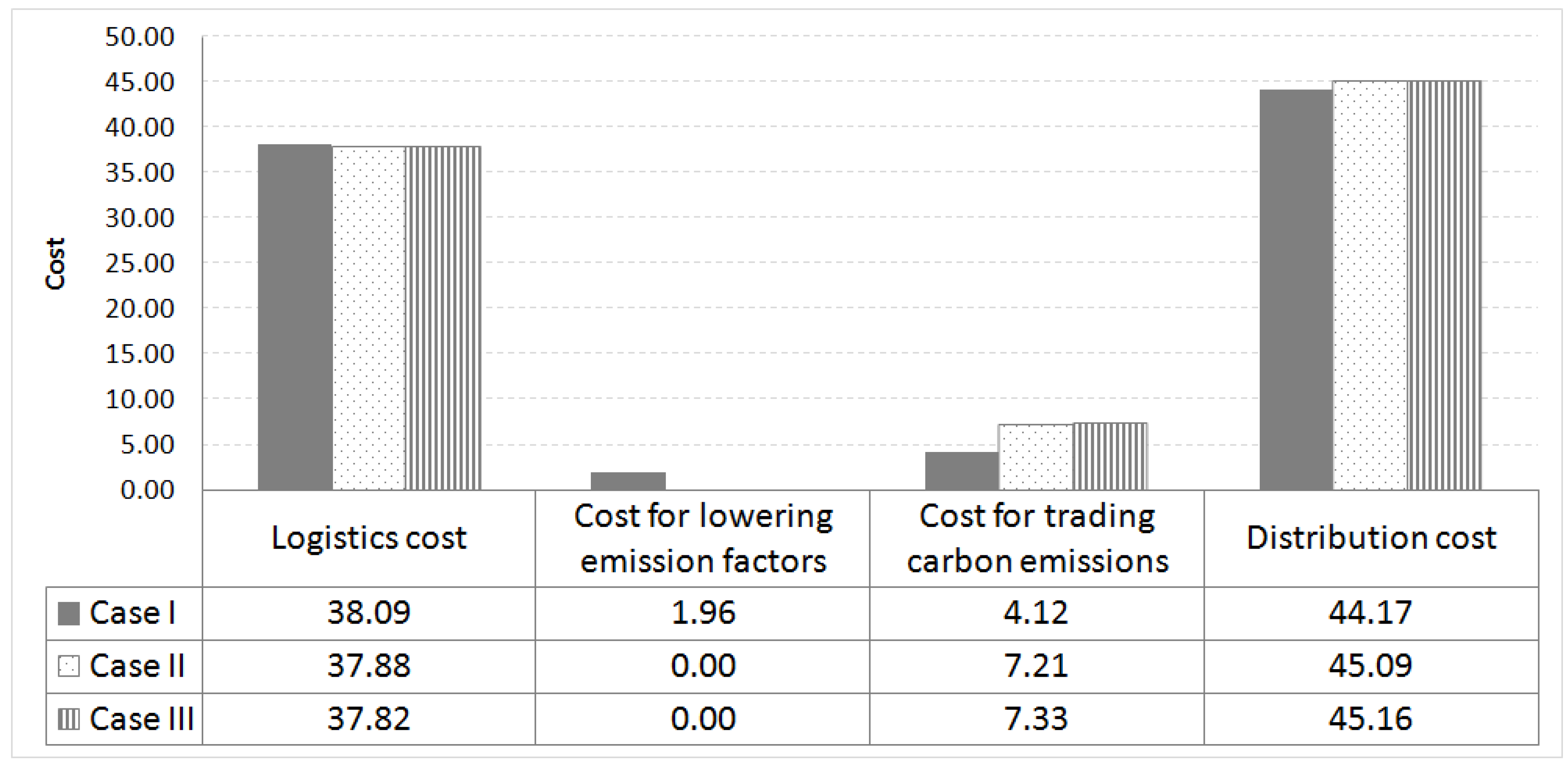
The detailed investigation of the distribution cost explains the effects of adjusting emission factors on reducing the distribution cost that is the sum of the logistics cost (i.e., traditional transportation and inventory holding cost), cost for lowering carbon emission factors and cost for trading carbon emissions. Figure 5 divides the distribution cost into three cost components so as to show which one of them mainly affects the reduction of the distribution cost. In Figure 5, Case I describes a situation where emission factors are adjusted to their optimal levels. Unlike Case I, we keep the initial values of emission factors and make no change in and in both Case II and Case III. Case II shows an optimal shipment size with the cost associated with carbon emissions, whereas Case III totally ignores carbon costs when determining an optimal shipment size. Thus, Case I, Case II and Case III result in an optimal shipment size as , , and , respectively.
While Case I has a higher logistics cost compared with two other cases, it successfully minimizes the distribution cost by significantly saving costs for trading carbon emissions. Case I has an additional cost for lowering emission factors, but the adjustment of emission factors helps save more in costs for trading carbon emissions, and the distribution cost becomes less than the other cases (see Theorem 3). Thus, we believe that this result supports the feasibility of making an investment in lowering carbon emission factors.
We further investigate the amount of carbon and cost reduction under the peddling strategy and summarize the results in Table 4, where and represent carbon and cost reductions, respectively. Recall that the optimal shipment size is fixed as U, and there is no condition on reducing carbon emissions and distribution cost. The effects of the vehicle capacity U are now investigated rather than evaluating the sensitivity of the ratio .
It should be noted that the carbon emission with optimal emission factors dramatically goes up to 31.73 from 9.05 when U moves from 8 to 9. This change in U switches optimal emission factors from to , which leads to a significant increase of carbon emissions. As aforementioned, reducing the carbon emission is allowed only when the cost for lowering emission factors is less than the benefit from reducing carbon emissions. In this numerical example, a sufficiently large vehicle capacity reduces the benefits from reducing relevant cost than lowering carbon emissions. Thus, a large shipment size is better in terms of lowering carbon emissions, but the shipment size should be limited as above to pursue lowering carbon emissions and minimizing the distribution cost.
7. Conclusions
This paper proposes a model for a joint decision on the shipment size and emission factors under two distribution strategies: direct shipment and peddling strategies. Analytical and numerical investigation provides some interesting findings. First, the policy for determining emission factors is of a control limit-type with respect to the unit cost for lowering emission factors. In particular, the optimal emission factors in transportation and warehousing are interdependent with each other. Comparing the two distribution strategies indicates that peddling strategy should give relatively more focus to transportation than warehousing in terms of lowering the emission factors. On the contrary, the chance of lowering the emission factor in warehousing is higher under the direct shipment strategy. A sufficient reduction in the distribution cost enables lower emission factors, whereas it incurs additional investment cost. Further analysis shows the possibility of reducing the carbon emissions and distribution costs by adjusting the shipment size along with lowering the emission factors. Finally, the numerical analysis validates the analytical results.
The results give us some interesting directions for future research. First, we consider that the cost for lowering carbon emissions is a linear function of carbon reduction; however, some papers in the literature formulate the cost as a quadratic function. It is arguable whether one should use a linear or convex function to formulate the cost incurred by reducing carbon emissions. Nevertheless, it is interesting to extend the current linear cost function for lowering carbon emission factors to a convex cost function. As aforementioned, considering a convex function removes the concavity of the distribution cost, and optimal emission factors should be numerically identified. For that purpose, investigating structural properties is required to design and improve an effective procedure for identifying the optimal emission factors.
This paper considers two types of distribution systems and briefly describes the similarities and differences in how to adjust the shipment size and emission factors to minimize the distribution cost. It is of interest to compare the two distribution strategies in terms of carbon and cost reductions. This comparison will provide insights on designing a cost-effective distribution system.
References
Acknowledgments
This work was supported by the Ministry of Education of the Republic of Korea and the National Research Foundation of Korea (NRF-2017S1A5A8021668).
Author Contributions
Daiki Min proposed the main idea of the paper motivated by the previous research. Daiki Min and Kwanghun Chung developed mathematical models and obtained optimal solutions for them. Daiki Min performed numerical analysis for the solution. All authors wrote and revised the paper.
Conflicts of Interest
The authors declare no conflict of interest.
References
- International Carbon Action Partnership (ICAP). Emission Trading Worldwide: ICAP Status Report; ICAP: Berlin, Germany, 2015. [Google Scholar]
- World Economic Forum (WEF). Supply Chain Decarbonisation: The Role of Logistics and Transport in Reducing Supply Chain Carbon Emissions; World Economic Forum: Geneva, Switzerland, 2009. [Google Scholar]
- Intergovernmental Panel on Climate Change (IPCC). Climate Change 2007: Mitigation; IPCC: Geneva, Switzerland, 2007. [Google Scholar]
- World Business Council for Sustainable Development (WBCSD). Mobility 2030: Meeting the Challenges to Sustainability; WBCSD: Geneva, Switzerland, 2004. [Google Scholar]
- Hua, G.; Cheng, T.; Wang, S. Managing carbon footprints in inventory management. Int. J. Prod. Econ. 2011, 132, 178–185. [Google Scholar] [CrossRef]
- Chen, X.; Benjaafar, S.; Elomri, A. The carbon-constrained EOQ. Oper. Res. Lett. 2013, 41, 172–179. [Google Scholar] [CrossRef]
- Bouchery, Y.; Ghaffari, A.; Jemai, Z.; Dallery, Y. Including sustainability criteria into inventory models. Eur. J. Oper. Res. 2012, 222, 229–240. [Google Scholar] [CrossRef]
- Benjaafar, S.; Li, Y.; Daskin, M. Carbon footprint and the management of supply chains: Insights from simple models. IEEE Trans. Autom. Sci. Eng. 2013, 10, 99–116. [Google Scholar] [CrossRef]
- Bouchery, Y.; Ghaffari, A.; Jemai, Z.; Tan, T. Impact of coordination on costs and carbon emissions for a two-echelon serial economic order quantity problem. Eur. J. Oper. Res. 2017, 260, 520–533. [Google Scholar] [CrossRef]
- Konur, D. Carbon constrained integrated inventory control and truckload transportation with heterogeneous freight trucks. Int. J. Prod. Econ. 2014, 153, 268–279. [Google Scholar] [CrossRef]
- Konur, D.; Schaefer, B. Economic and environmental comparison of grouping strategies in coordinated multi-item inventory systems. J. Oper. Res. Soc. 2016, 67, 421–436. [Google Scholar] [CrossRef]
- Jiang, Y.; Klabjan, D. Optimal Emissions Reduction Investment under Green House Gas Emissions Regulations. Working Paper. 2012. Available online: http://dynresmanagement.com/uploads/3/3/2/9/3329212/carbonregulations.pdf (accessed on 12 April 2016).
- Song, J.; Leng, M. Handbook of Newsvendor Problems: Models, Extentions and Applications; Springer: Berlin, Germany, 2012. [Google Scholar]
- Zhang, B.; Xu, L. Multi-item production planning with carbon cap and trade mechanism. Int. J. Prod. Econ. 2013, 144, 118–127. [Google Scholar] [CrossRef]
- Piecyk, M.; McKinnon, A. Forecasting the carbon footprint of road freight transport in 2020. Int. J. Prod. Econ. 2010, 128, 31–42. [Google Scholar] [CrossRef]
- Ballot, E.; Fontane, F. Reducing transportation CO2 emissions through pooling of supply networks: Perspective from a case study in French retail chain. Prod. Plan. Control 2010, 21, 640–650. [Google Scholar] [CrossRef]
- Lai, K.; Wong, C. Green logistics management and performance: Some empirical evidence from Chinese manufacturing exporters. Omega 2012, 40, 267–282. [Google Scholar] [CrossRef]
- Swami, S.; Shah, J. Channel coordination in green supply chain management. J. Oper. Res. Soc. 2013, 64, 336–351. [Google Scholar] [CrossRef]
- Dong, C.; Shen, B.; Chow, P.; Yang, L.; Ng, C. Sustainability investment under cap-and-trade regulation. Ann. Oper. Res. 2016, 240, 509–531. [Google Scholar] [CrossRef]
- Toptal, A.; Ozlu, H.; Konur, D. Joint decisions on inventory replenishment and emission reduction investment under different emission regulations. Int. J. Prod. Res. 2014, 52, 243–269. [Google Scholar] [CrossRef] [Green Version]
- Moon, I.; Jeong, Y.; Saha, S. Fuzzy Bi-Objective Production-Distribution Planning Problem under the Carbon Emission Constraint. Sustainability 2016, 8, 798. [Google Scholar] [CrossRef]
- McKinnon, A. Green logistics: The carbon agenda. LogForum 2010, 6, 1–9. [Google Scholar]
- Burns, L.; Hall, R.; Blumenfeld, D.; Daganzo, C. Distribution strategies that minimize transportation and inventory costs. Oper. Res. 1985, 33, 469–490. [Google Scholar] [CrossRef]
- Gallego, G.; Simchi-Levi, D. On the effectiveness of direct shipping strategy for the one-warehouse multi-retailer R-systems. Manag. Sci. 1990, 36, 240–243. [Google Scholar] [CrossRef]
- World Resources Institute (WRI). Technical Guidance for Calculating Scope 3 Emissions; WRI: Washington, DC, USA, 2013. [Google Scholar]
- Bouchery, Y.; Fransoo, J. Cost, carbon emissions and modal shift in intermodal network design decisions. Int. J. Prod. Econ. 2015, 164, 388–399. [Google Scholar] [CrossRef]
- Wang, S.; Tao, F.; Shi, Y.; Wen, H. Optimization of Vehicle Routing Problem with Time Windows for Cold Chain Logistics Based on Carbon Tax. Sustainability 2017, 9, 695. [Google Scholar] [CrossRef]
- McKinnon, A.; Cullinane, S.; Browne, M.; Whitening, A. Green Logistics: Improving the Environmental Sustainability of Logistics; Kogan Page: London, UK, 2010. [Google Scholar]
- FedEx. Connecting the World in Responsible and Resourceful Ways. 2016. Available online: http://about.van.fedex.com/newsroom/fedex-boosts-efforts-to-connect-the-world-in-responsible-and-resourceful-ways/ (accessed on 12 April 2016).
- Dey, A.; LaGuardia, P.; Srinivasan, M. Building sustainability in logistics operations: A research agenda. Manag. Res. Rev. 2011, 34, 1237–1259. [Google Scholar] [CrossRef]
- Min, D. Carbon reduction investment under direct shipment strategy. Manag. Sci. Financ. Eng. 2015, 21, 25–29. [Google Scholar] [CrossRef]
- Stein, D. Scheduling Dial-a-Ride transportation systems. Transp. Sci. 1978, 12, 232–249. [Google Scholar] [CrossRef]
- Kwon, H.; Seo, S. Korean Macroeconomic Logistics Costs in 2010; The Korea Transport Institute: Sejong-si, Korea, 2013. [Google Scholar]
- Korea Exchange. Busan, Korea, 2015. Available online: http://www.krx.co.kr (accessed on 12 April 2016).
Figure 1.
Optimal solution of direct shipment.

Figure 2.
Difference in carbon emissions and distribution cost. (a) difference with respect to F; (b) difference with respect to V; (c) difference with respect to H.
Figure 2.
Difference in carbon emissions and distribution cost. (a) difference with respect to F; (b) difference with respect to V; (c) difference with respect to H.
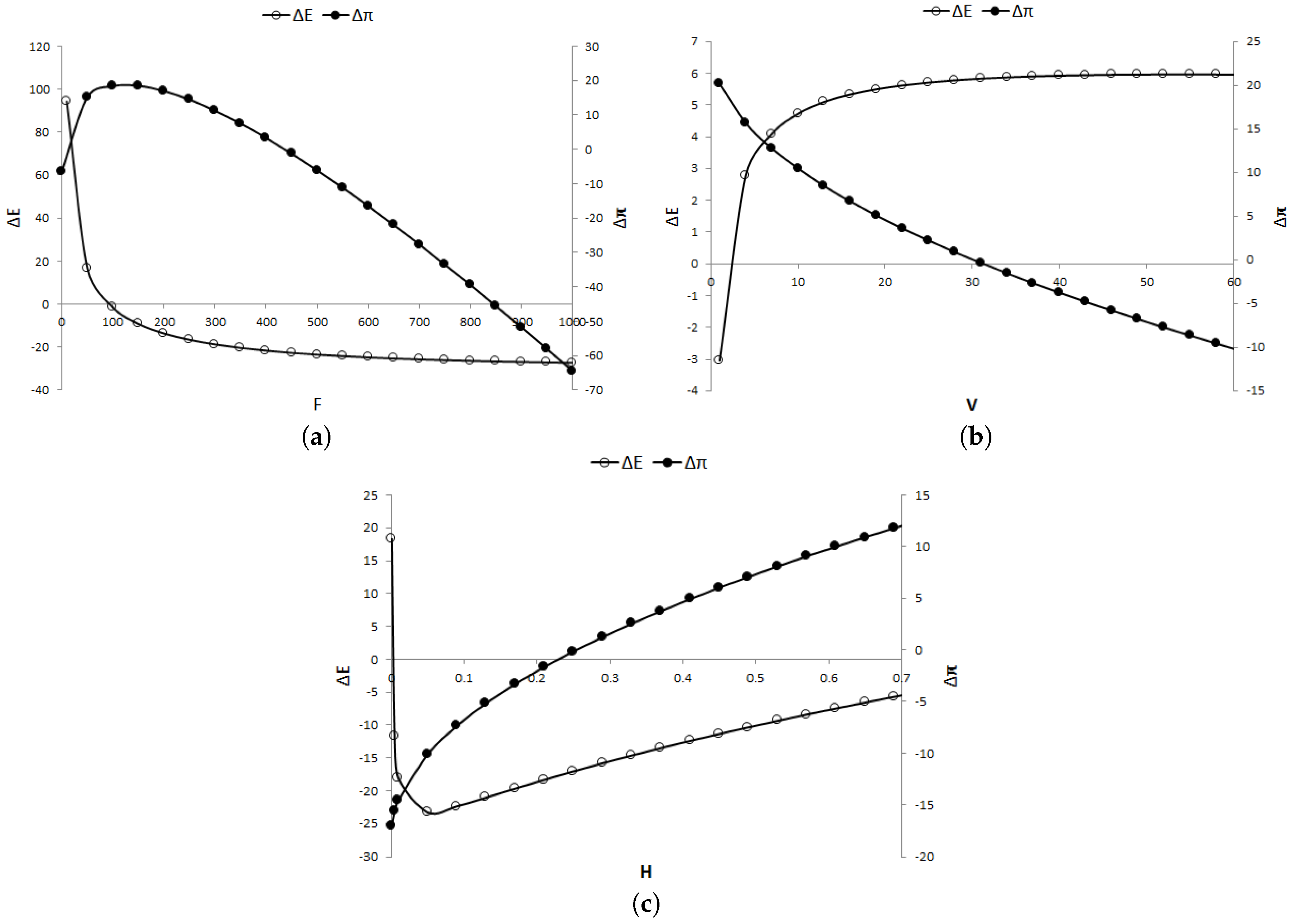
Figure 3.
with a cost function for lowering emission factors. (a) linear cost function; (b) quadratic cost function.
Figure 3.
with a cost function for lowering emission factors. (a) linear cost function; (b) quadratic cost function.

Figure 4.
Carbon emission reduction under the direct shipment strategy.
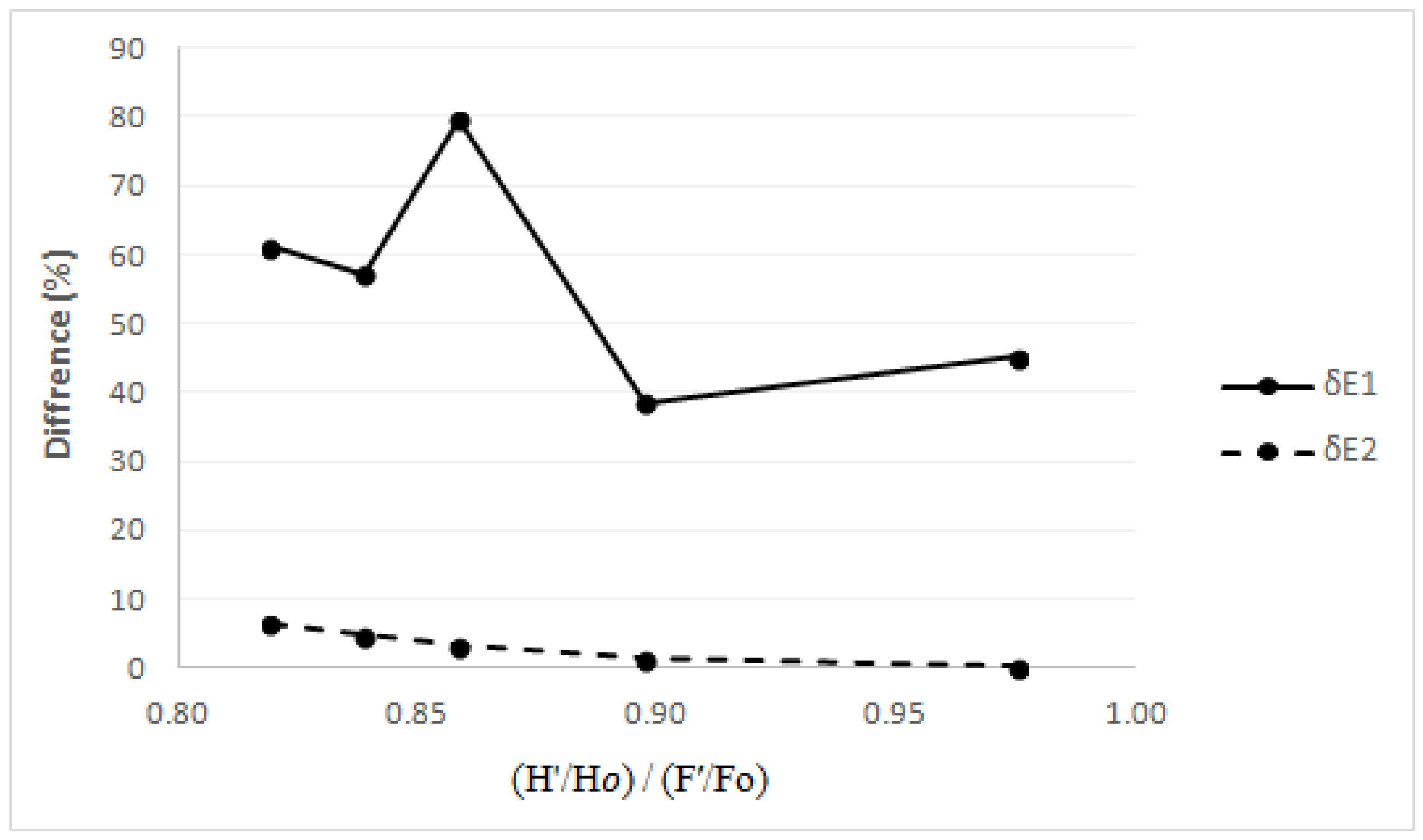
Figure 5.
Reducing the distribution cost.

Table 1.
Summary of notations.
| Notation | Description |
|---|---|
| Input data | |
| D | weekly customer demand (tonnes/customer) |
| inventory holding cost ($/tonne-week) | |
| L | round trip distance between depot and customer (km) |
| T | transit time between supplier to customer (weeks) |
| U | truck capacity (tonnes/truck) |
| fixed cost of initiating a truck dispatch ($/load) | |
| transportation cost ($/km) | |
| fixed cost of a customer visit ($/visit) | |
| carbon price ($/kgCO) | |
| K | carbon emission cap per unit (kgCO/tonne) |
| unit cost for lowering the emission factor in transportation ($/kgCO/km) | |
| unit cost for lowering the emission factor in warehousing ($/kgCO) | |
| Decision variables | |
| q | shipment size (tonnes/load) |
| x | the amount of carbon trading per unit (kgCO /tonne) |
| c | emission factor in transportation (kgCO/tonne-km) |
| h | emission factor in warehousing (kgCO/tonne-week) |
Table 2.
Finding , , , (, , , ).
| Direct Shipment (, ) | Peddling (, ) | ||||||||||||
|---|---|---|---|---|---|---|---|---|---|---|---|---|---|
| 0.2 | 3.59 | 3.47 | 1.48 | 1.35 | 2.51 | 2.50 | 0.28 | 0.26 | |||||
| D | 0.4 | 2.54 | 2.46 | 1.05 | 0.96 | 2.36 | 2.35 | 0.19 | 0.18 | ||||
| 0.6 | 2.07 | 2.01 | 0.85 | 0.78 | 2.30 | 2.29 | 0.16 | 0.15 | |||||
| 0.05 | 1.83 | 1.80 | 0.71 | 0.67 | 1.26 | 1.25 | 0.13 | 0.13 | |||||
| 0.1 | 3.59 | 3.47 | 1.48 | 1.35 | 2.51 | 2.50 | 0.28 | 0.26 | |||||
| 0.15 | 5.29 | 5.04 | 2.32 | 2.04 | 3.76 | 3.72 | 0.43 | 0.39 | |||||
| % | 10 | 3.60 | 3.49 | 1.47 | 1.35 | 2.52 | 2.50 | 0.27 | 0.26 | ||||
| reduction in | 20 | 3.61 | 3.51 | 1.45 | 1.36 | 2.51 | 2.50 | 0.27 | 0.26 | ||||
| and | 30 | 3.62 | 3.53 | 1.44 | 1.36 | 2.51 | 2.50 | 0.27 | 0.26 | ||||
Table 3.
Evaluation of carbon and cost reduction under the direct shipment strategy.
| Carbon Reduction Investment | Carbon Consideration but No Reduction | No Carbon Consideration | |||||||
|---|---|---|---|---|---|---|---|---|---|
| 0.82 | 2.20 | 39.24 | 72.57 | 2.40 | 101.23 | 75.34 | 2.18 | 108.25 | 75.71 |
| 0.84 | 2.66 | 38.75 | 60.40 | 2.91 | 90.56 | 62.03 | 2.66 | 95.04 | 62.28 |
| 0.86 | 3.17 | 17.35 | 53.03 | 3.32 | 85.13 | 54.21 | 3.08 | 88.08 | 54.37 |
| 0.90 | 4.24 | 49.24 | 44.17 | 3.98 | 80.11 | 45.09 | 3.77 | 81.34 | 45.16 |
| 0.98 | 5.00 | 42.50 | 34.69 | 4.92 | 77.55 | 36.23 | 4.86 | 77.60 | 36.23 |
Table 4.
Evaluation of carbon and cost reduction under peddling strategy.
| U | Carbon Investment | No Reduction | Difference | |||
|---|---|---|---|---|---|---|
| 5 | 12.80 | 29.46 | 53.84 | 31.56 | 320.51 | 7.16 |
| 6 | 11.14 | 26.91 | 47.17 | 28.27 | 323.57 | 5.05 |
| 7 | 9.95 | 25.09 | 42.41 | 25.91 | 326.40 | 3.28 |
| 8 | 9.05 | 23.72 | 38.84 | 24.14 | 329.00 | 1.77 |
| 9 | 31.73 | 22.46 | 36.06 | 22.77 | 13.65 | 1.36 |
| 10 | 29.51 | 21.36 | 33.84 | 21.67 | 14.68 | 1.43 |
; .
© 2017 by the authors. Licensee MDPI, Basel, Switzerland. This article is an open access article distributed under the terms and conditions of the Creative Commons Attribution (CC BY) license (http://creativecommons.org/licenses/by/4.0/).
Share and Cite
MDPI and ACS Style
Min, D.; Chung, K. A Joint Optimal Decision on Shipment Size and Carbon Reduction under Direct Shipment and Peddling Distribution Strategies. Sustainability 2017, 9, 2061. https://doi.org/10.3390/su9112061
AMA Style
Min D, Chung K. A Joint Optimal Decision on Shipment Size and Carbon Reduction under Direct Shipment and Peddling Distribution Strategies. Sustainability. 2017; 9(11):2061. https://doi.org/10.3390/su9112061
Chicago/Turabian StyleMin, Daiki, and Kwanghun Chung. 2017. "A Joint Optimal Decision on Shipment Size and Carbon Reduction under Direct Shipment and Peddling Distribution Strategies" Sustainability 9, no. 11: 2061. https://doi.org/10.3390/su9112061
Note that from the first issue of 2016, this journal uses article numbers instead of page numbers. See further details here.