The Environmental Conservation Value of the Saemangeum Open Sea in Korea

Abstract

The Saemangeum open sea (SOS), which refers to the outer sea of the Saemangeum seawall in Korea, is being threatened by contamination caused by the Saemangeum development project. The policy-makers need information on the environmental conservation value of the SOS for informed decision-making about the SOS. This paper attempts to measure the environmental conservation value of the SOS. To this end, the public’s willingness to pay (WTP) for conserving the SOS is derived from a 2015 contingent valuation survey of 1000 Korean households comprising 400 households residing in the Saemangeum area and 600 households living in other areas. The authors employ a one-and-one-half-bounded dichotomous choice question format. Moreover, the spike model is adopted to analyze the WTP data with zero observations. The mean annual WTP values for both areas are calculated to be KRW 3861 (USD 3.26) and KRW 3789 (USD 3.20) per household, respectively. They are statistically significant at the 1% level. When the sample is expanded to the whole country, it is worth KRW 70.9 billion (USD 59.8 million) per annum. Therefore, conserving the SOS will contribute to the Korean people’s utility and can be done with public support. The value provides a useful baseline for decision-making for the SOS management.

1. Introduction

Saemangeum is an estuarine tidal flat in the western coastal area of the Korean Peninsula. It was dammed due to the Saemangeum seawall construction project carried out by the Korean government. The Saemangeum seawall is located on the coast of the Korean West Sea (near Gunsan, Gimjae and the Buan areas of Jeonbuk Province); at 33 km long, it is the world’s longest man-made dyke. It was constructed for the purpose of developing reclaimed land of 40,100 ha and providing a freshwater lake for agriculture.

Since the seawall was constructed, the Saemangeum sea area has been divided into the freshwater lake and the outside open sea, the Saemangeum open sea (SOS). The government began developing the reclaimed land. Although the original plan was for the development of farmland, the project now includes not only farmland, but also industrial, commercial, and residential areas. Thus, the proportion of farmland was changed from 100% to 34%. In addition, the Saemangeum development project includes the construction of tourist facilities and new ports in the SOS. Unfortunately, Korea has not yet reached a social consensus on the magnitude of the benefits and costs involved in the project. The local governments in the Saemangeum area have strongly supported the project. This is because the Korean government will invest trillions of Korean won (billions of United States dollar) in the project and the Saemangeum area is thus expected to obtain economic gains such as the creation of new jobs, expansion of social infrastructure, the influx of an economically active population, and so on, if it decides to carry out the project. However, the project will negatively influence the ecological integrity of the Saemangeum area. In summary, the Saemangeum area can benefit from the development but will shoulder a burden of the environmental costs to the SOS caused by the development.

The Saemangeum development project will exacerbate the water pollution of the SOS. This is because the freshwater lake, polluted from industrial and agricultural emissions, will flow into the SOS [1]. The pollution will make it difficult for people to pursue ocean recreation activities such as fishing, boat tours, watching the scenic view, and so on. In addition, the project will negatively influence marine ecosystem services that the SOS provides. The project will weaken its ability to sustain the marine biodiversity of the habitat. For example, the Spoon-billed Sandpiper (Calidris pygmaea) that lives in the SOS may become extinct. Moreover, a mass mortality of Finless Porpoises (Neophocaena asiaeorientalis) may occur for some unknown reason around the Saemangeum seawall.

There are still conflicts about the development. Some are interested in preserving the ecological integrity of the SOS, and others want to develop the Saemangeum area and attract tourists and capital investments using the seawall. Thus, the government is confronted with two important tasks. The first is to mediate between the opponents and the proponents for the development and set up sustainable development plans for the Saemangeum area. The second is to create the SOS management policy. In fulfilling the two tasks, information on the environmental conservation value of the SOS is required by policy-makers. Therefore, this study attempts to report the results of estimating the environmental conservation value of the SOS.

Currently, the state of the SOS is relatively good. However, the artificial seawall is expected to degrade the water quality of the Saemangeum lake inside the seawall, and will thus negatively affect the ecological integrity of the SOS in the near future [2]. In order to avoid the deterioration and conserve the ecological integrity of the SOS, policies for effective management of the SOS should now be developed and implemented. There is a general lack of awareness about the conservation of the SOS although people should prepare response measures to prevent the negative effect on the marine environment due to developing the reclaimed land . In this situation, this study has tried to quantify the monetary value of the current state of the SOS. In order for policy-makers to mediate between opponents and proponents of the development, set up sustainable development plans for the Saemangeum area, and create the SOS management policy, information on the environmental conservation value of the SOS is required [3,4].

Therefore, the prime objective of this article is to add a contribution to the existing literature by measuring the environmental conservation value of the SOS. For this purpose, the article attempts to adopt the contingent valuation (CV) technique to derive the public’s willingness to pay (WTP) for conserving the SOS. The public’s WTP can be interpreted as the environmental conservation value of the SOS [5,6]. The rest of the article comprises four sections: the methodology employed in the study, the WTP model, the results and a discussion of them, and conclusions.

2. Methodology

2.1. CV Method

The task of dealing with the valuation of the marine ecosystem falls to researchers. There have been a number of studies dealing with the valuation of marine ecosystems. The literature shows that such tasks have been conducted using stated preference techniques, including CV (e.g., [7,8,9,10,11]) and choice experiments (e.g., [12,13,14]). On the other hand, Camacho-Valdez et al. [15] generate baseline estimates of the ecosystem services provided by wetlands using value transfer approach. Ruitenbeek [16] used a market value approach to value a mangrove. This study seeks to examine the environmental conservation value of the SOS using the CV approach.

Conserving the SOS should be understood as a case of public goods. In terms of microeconomics, the public’s WTP for a governmental plan or policy constitutes the underpinning rule for the public value that ensues from undertaking the plan or policy. However, as public goods are not traded on the market, the WTP for its provision cannot be observed in the market. Public goods are representative of non-market goods. Thus, to measure the public’s WTP for public goods, it is necessary to construct a hypothetical market, immerse people in the hypothetical market, and have people trade in the hypothetical market. The CV approach can carry out these procedures based on a well-organized survey of people using a well-constructed instrument and well-trained interviewers. CV is the technique most frequently applied in the literature and can easily capture compensating surplus, which is defined as the welfare gain generated from greater provision or an improvement in the quantity or quality of non-market goods. Moreover, because the value obtained from the application of CV implies the economic benefits of consuming the public goods, one can evaluate whether the provision of the public goods is socially profitable by comparing it with the costs of providing the public goods. Thus, we use the CV technique to evaluate Koreans’ WTP for conserving the SOS in Korea [17,18].

This study can be compared with the former studies in several aspects. First, there have been no studies that measure the environmental conservation value of the SOS in the literature. In this regard, this study attempts to provide quantitative information on the environmental conservation value of the SOS, which can be utilized in decision-making for the SOS management, with policy-makers. The information can be used as an appropriate and important reference point for a more detailed discussion.

Second, the most widely applied technique in the valuation of the marine ecosystem is the CV technique. Thus, our approach of employing the CV in valuing the environmental conservation of the SOS is appropriate judging from the practice adopted in the previous studies. Moreover, Arrow et al. [19] strongly recommended the application of the CV method in circumstances requiring administrative and/or jurisdictional decision-making [20,21].

Third, this study tries to follow a number of recommendations raised by Arrow et al. [19] and in the literature in applying the CV approach. For example, Arrow et al. [19] suggested the use of at least 1000 observations, the use of in-person interviewing rather than telephone or mail interviewing, the use of close-ended questions instead of open-ended questions, reminding the respondents of substitutes for the goods to be valued, and so on. All these suggestions were performed in our study, as will be explained below. In addition, the authors used an annual payment in eliciting the respondent’s WTP, reflecting the suggestion of Egan et al. [22].

Fourth, this study performs a more careful consideration of inefficiency and response bias. The single-bounded (SB) question and the double-bounded (DB) question formats have been criticised in the literature because of statistical inefficiency caused by the use of the responses to just one question and response bias caused by a false response to the second question, respectively. Therefore, this study will apply a recently proposed elicitation method, which is known to reduce inefficiency and response bias, rather than SB question or DB question formats. Furthermore, this study handles zero WTP responses more carefully using the spike model, as will be described below in detail. Consequently, this study employs a combination of a recently developed elicitation method and the spike model.

Fifth, we divided the study area into two categories: on- and off-site areas. For this, 40% of the sample was randomly assigned in the area surrounding the SOS (the on-site area); the other 60% was allocated to the rest of the country (the off-site area). As explained above, the sample size was 1000. Sampling based on a regional population inevitably gives us quite a small size of the sample for the on-site area as the ratio of residents in the SOS area to the national population is very small. If simple random sampling based on population characteristics is implemented, the on-site residents’ concerns about and interests in the SOS cannot be adequately reflected in the CV survey. Thus, this study performs over-sampling for the on-site area and analyzes the WTP data by separately using the two samples. This is an interesting feature of our study.

2.2. Sampling

A random sampling method was commissioned from an expert who was affiliated with a professional survey firm; the sampling reflected the population characteristics observed from a census by Statistics Korea [23], the Korean National Statistical Office. More specifically, stratified random sampling was conducted. The survey firm performed a random sampling and field CV survey during September 2015. According to Statistics Korea, there were 18,705,004 households in Korea in 2015. In order to draw a random sample of this population, stratified random sampling was conducted by the polling firm. This included two steps. First, we decided to divide the entire sample into two samples of the on-site area and the off-site area. That is, a survey of 1000 Korean households comprising 400 households living in the Saemangeum area and 600 households living in other areas was implemented. The on-site area has three strata: Gunsan, Gimjae, and Buan. The off-site area has fifteen strata: Seoul, Busan, Daegu, Incheon Gwangju, Daejeon, Ulsan, Gyunggi, Gangwon, Chungbuk, Chungnam, Jeonbuk, Jeonnam, Gyungbuk, and Gyungnam. Second, a random sampling was conducted within each stratum.

In the case of the on-site sample, the sizes of the stratum for Gunsan, Gimjae, and Buan were 248, 92, and 60, respectively. As for the off-site sample, the sizes of stratum for Seoul, Busan, Daegu, Incheon Gwangju, Daejeon, Ulsan, Gyunggi, Gangwon, Chungbuk, Chungnam, Jeonbuk, Jeonnam, Gyungbuk, and Gyungnam were 137, 47, 32, 35, 20, 20, 11, 146, 16, 14, 19, 20, 14, 31, and 38, respectively. Each size of stratum was determined based on the population size of each stratum reported in the “2015 National Census on Population” conducted by Statistics Korea. The sampling within each stratum reflected each stratum’s population characteristics such as age, income, and gender. The trained interviewers carried out 1000 personal interviews at the interviewees’ homes.

The head or housekeeper of the sampled households was selected as the interviewee to derive responsible opinions from the perspective of a household rather than an individual. In addition, we limited the respondents’ age to 20–64 years including the working age population, because people who are younger or older have difficulties in responsibly responding to the WTP question [4,5,10,20,24,25,26,27,28].

2.3. Method of Eliciting WTP: Dichotomous Choice (DC) Question

We employed a DC question format for the purpose of obtaining the information on the respondents’ WTP. DC questions can mitigate protest bid responses and induce incentive-compatible responses. Using the DC question, an interviewee is asked to state whether she/he is willing to pay an offered bid to conserve the SOS and her/his response to the question is “yes” or “no.” If the response is “yes”, her/his WTP for conserving the SOS is higher than the bid. If the response is “no”, her/his WTP for conserving the SOS is lower than the bid. Specifically, the one-and-one-half-bounded (OOHB) DC question method presented in Cooper et al. [29] is employed in this study. This is because it can selectively exploit the merits of a SB DC format endorsed by Carson et al. [30] and a DB DC format suggested by Hanemann et al. [31].

In particular, the SB DC question or DB DC question is usually used. The SB DC question is a one-time DC question. On the other hand, the DB DC question employs two DC questions. The respondent who states “yes” to a first bid is additionally asked a follow-up question of whether she/he would pay a second, higher bid. A respondent who answers “no” to the first bid is additionally asked a follow-up question of whether she/he would pay a second lower bid.

The DB DC question format can significantly increase the statistical efficiency rather than the SB DC question format [31]. However, the DB DC question format also augments the response bias when compared to the SB DC question format (e.g., [30,32,33]). Thus, SB DC and DB DC questions suffer from low statistical efficiency and high response bias, respectively. As an alternative, Cooper et al. [29] suggested the OOHB DC question format. The statistical efficiency of the OOHB DC question format is similar to that of the DB DC question format, and the consistency of the OOHB DC question format is close to that of the SB DC question format.

The bids were determined in the following manner. From a focus group survey of directly asking for the respondent's WTP in an open-ended question, an empirical distribution of WTP was derived. Then, after trimming fifteen percent from both tails of the WTP distribution, we obtained a list of possible bids from the remaining WTP distribution. Finally, $S$ sets of bids to be presented to respondents were decided following two principles given in Cooper et al. [29]. The first principle is that a set should comprise two bids (lower and upper bids). The second principle is that a set of bids should partially overlap with the next set of bids. For example, when a set of bids is (USD 2, USD 6), the next set of bids is (USD 4, USD 8), where the first and the second elements are the lower and higher bids, respectively. The former higher bid is larger than the latter lower bid. A set among $S$ sets was randomly allocated to each respondent. From the results from a focus group interview, the list of bids was determined as KRW 1000/3000, 2000/4000, 3000/6000, 4000/8000, 6000/10,000, 8000/12,000, and 10,000/15,000. When the survey was conducted, the exchange rate was USD 1.0 = KRW 1185.

2.4. Payment Vehicle

A payment vehicle to immerse people in the hypothetical situation was needed for the CV question. In this regard, tax can be preferred to a donation or a fund for several reasons. First, a payment vehicle should be persuasive and understandable to the respondents. A number of Korean people do not feel at home with a donation or a fund because only a small number of persons pay money in the form of a donation or a fund. On the other hand, Korean people currently pay a variety of taxes. Thus, a tax is more persuasive and understandable to the respondents than a donation or a fund. Second, a payment vehicle should be familiar to the respondents to avoid any problems involved in a hypothetical question. The use of a donation or a fund as a payment vehicle rather than tax deepens a hypothetical condition which the respondents are confronted with. Third, the goods to be valued should have a clear connection with the payment vehicle. A tax is more related with the conservation of the SOS than a donation or a fund. This is because the public will absorb the costs that will be paid for its implementation by taxes if the conservation of the SOS is implemented.

The authors employed the vehicle of income tax, because in Korea income tax is the most common among several taxes. Two more points to be decided were the payment frequency and period. Following the recommendation of Egan et al. [22], we used an annual payment. The payment period was then determined to be 10 years, reflecting the practices of previous CV studies conducted in Korea (e.g., [21,25]).

2.5. Survey Instrument

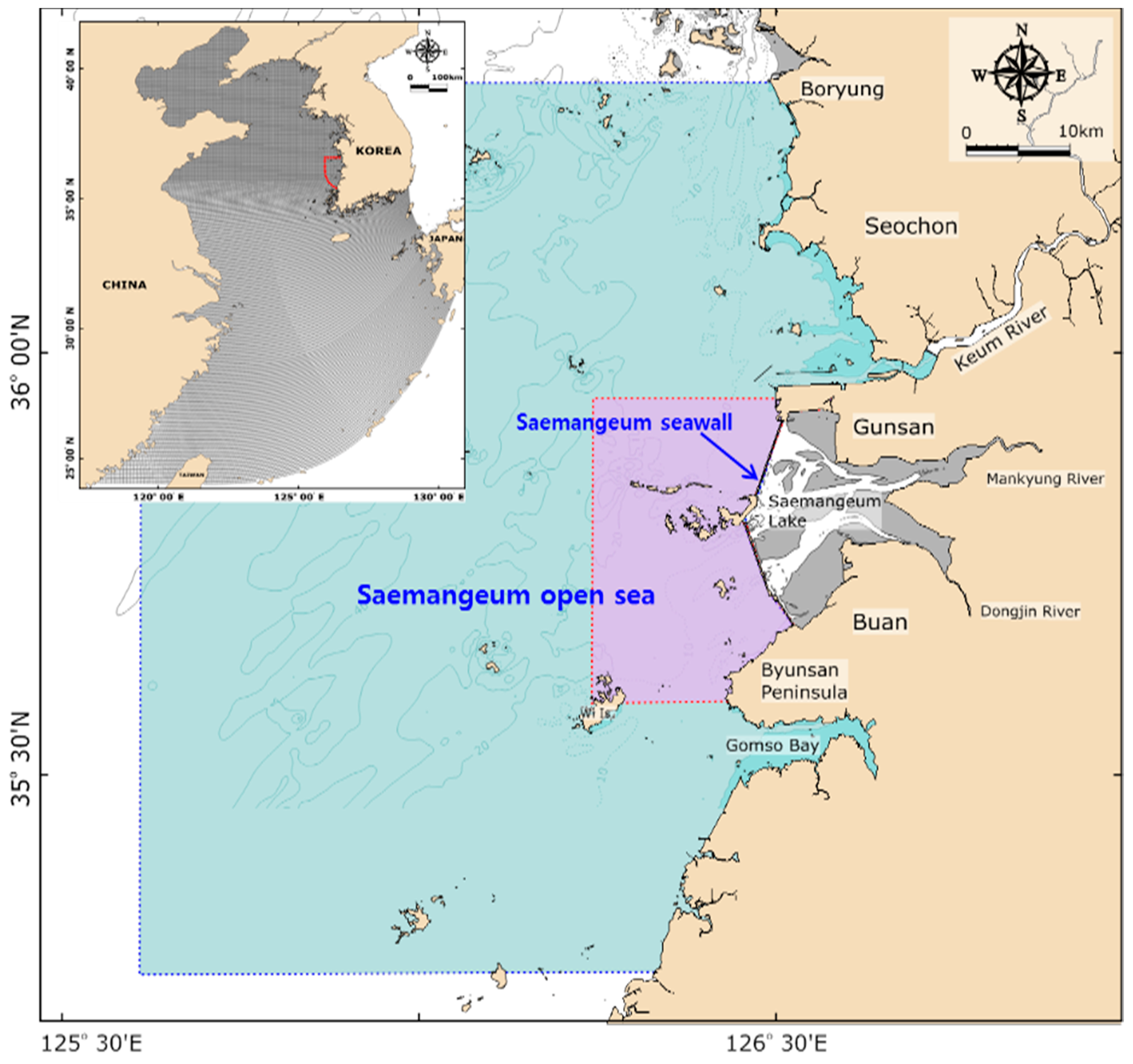
CV is a standardized and widely-used survey method for estimating WTP, involving constructing a hypothetical market or referendum scenario in a survey. The proposed implementation (if respondents pay) or non-implementation (if respondents do not pay) in the quantity or quality of the goods is communicated to respondents in words and with visual aids. For example, the geographical location of the SOS area and seawall, shown in Figure 1, was presented in the survey. Next, respondents are informed of how they will pay for the proposed quantity or quality. Then, the provision rule is made clear: if you agree to pay, you get the proposed quantity or quality; if you do not pay, you do not get the proposed quantity or quality level. Respondents use the hypothetical market to state their WTP or vote for or against the goods.

A preliminary survey questionnaire was tested with a focus group of thirty individuals to ascertain its understandability and clarity. Reflecting the results of the focus group, we finalized the CV survey instrument to include the following: (a) an introduction section to explain background information and descriptions of the objective; (b) questions concerning respondents’ perceptions and experiences related to the object to be valued; (c) a scenario in which conserving the SOS to be valued would be provided to the public and should be clearly explained and questions about the annual WTP for conserving the SOS; and (d) questions regarding the characteristics of the respondents’ household.

The WTP question asked in the CV survey was “Does your household have the willingness to pay a specified bid for conserving the Saemangeum open sea through an increase in yearly income tax, supposing that the conservation would certainly be implemented?” The policy instruments for the conservation include preventing the reckless development of the SOS, increasing the governmental investments on research and development of the SOS conservation technology, and continuously monitoring and investigating the SOS. Additional statements regarding payment were provided. The policy instruments were explicitly presented in the survey questionnaire. The interviewers urged the respondents to read the survey questionnaire aloud and prompted them to ask any questions about the policy instruments.

For example, the interviewees were asked: “Currently policymakers need information on the environmental conservation value of the SOS to make an informed decision about whether and how to invest in the conservation. When the conservation is promoted, the public will pay national taxes to carry out the conservation. Since there will be a financial burden if the conservation proceeds, the public support will be necessary to carry it out successfully. As it is vital to obtain public agreement for this intensive financing, the public’s acceptance of the conservation should be examined. If there is a preponderance of negative responses regarding the conservation, the conservation cannot be carried out. However, in the case of objections, the conservation can be implemented. Please keep in mind that your household’s income is constrained and that there are various expenditures in your household.”

3. WTP Model

3.1. OOHB DC Model

The following model comes from Cooper et al. [29]. Let $T$, $A_j$, and $Y_j$ be the number of observations, the bid offered to respondent $j$, and respondent $j$’s WTP, respectively. Before conducting the CV survey, sets of two bids, $A_j^L$ and $A_j^U$ ($A_j^L<A_j^U$), should be determined. In the field survey, a set is randomly offered to respondent $j$ in the following manner. About fifty percent of respondents are confronted with $A_j^L$ and asked to decide whether they are willing to pay $A_j^L$. If their answer is “yes”, they are additionally faced with $A_j^U$ and required to state “yes” or “no” to $A_j^U$. If they say “no” to $A_j^L$, no further question is asked. Similarly, remaining respondents are provided with $A_j^U$ and urged to decide whether they are willing to pay $A_j^U$. If the answer is “no”, an additional question concerning $A_j^L$ is asked. If they say “yes” to $A_j^U$, no further question is presented.

Methodologically, about 50% of respondents are confronted with ascending bids and about 50% see descending bids. There are two reasons for the use of this control. First, the control has been used in the literature since Cooper et al. [29], who originally designed the OOHB DC model. Second, the control is useful in neutralizing or weakening the impact of the order of bids on the responses to a given bid. The list of possible responses when $A_j^L$ is offered at first are “yes-yes” ($Y_j>A_j^U$), “yes-no” ($A_j^L<Y_j<A_j^U$), and “no” ($Y_j<A_j^L$). Likewise, the list of possible responses when $A_j^U$ is supplied at first are “yes” ($Y_j>A_j^U$), “no-yes” ($A_j^L<Y_j<A_j^U$), and “no-no” ($Y_j<A_j^L$). Thus, the variables describing the six responses are formulated as $I_j^{YY}$, $I_j^{YN}$, $I_j^N$, $I_j^Y$, $I_j^{NY}$, and $I_j^{NN}$, for which the value is one if interviewee $j$’s answer coincides with the superscript and zero if not.

3.2. Spike Model

A number of persons may have zero WTP for conserving the SOS. From an economic perspective, the zero WTP can arise as a corner solution to the problem of utility maximization under income constraint. A total of 54.0% of the on-site sample respondents and 56.3% of the off-site sample respondents reported zero WTP, respectively, as will be explained in Section 4.1. The modeling of WTP responses should reflect both the positive WTP responses and the zero WTP responses. As discussed above, one model that we can apply to analyze the WTP data with zero observations is a spike model given in Kriström [34] and Yoo and Kwak [35]. Thus, this study utilizes the spike model to handle the WTP observations with a number of zeros.

An additional question identifying respondents’ WTP as a positive value less than the lower bid ($A_j^L$) or zero was asked of the respondents who stated “no” to the lower bid. The possible responses are “yes” and “no.” The former means $0<Y_j<A_j^L$, and the latter indicates $Y_j=0$. Consequently, one more binary variable, $I_j^{TY}$, can be defined. Its value is one if respondent $j$ responded “yes” to the additional question and zero otherwise.

In the spike model, we formulate the distribution function of the WTP, $H_Y(\cdot )$, as follows:

$$H_Y(A;{\gamma }_0,{\gamma }_1)=\{\begin{array}{ll}{[1+\exp ({\gamma }_0-{\gamma }_{1}A)]}^{-1}& \hfill \mathrm{if}A>0\\ {[1+\exp ({\gamma }_0)]}^{-1}& \hfill \mathrm{if}A=0\\ 0& \hfill \mathrm{if}A<0\end{array}$$

(1)

where ${\gamma }_0$ and ${\gamma }_1$ are the parameters of the WTP distribution.

The spike, defined as the probability of the respondent having zero WTP is computed as $1/[1+\exp ({\gamma }_0)]$. The probability of the respondent’s WTP being negative is assumed to be zero. The last condition does imply that negative WTP is not allowed. Of course, the negative WTP may exist in the form of a subsidy. However, in actuality, any subsidy for the respondents with negative WTP cannot occur in the situation of Korea. Thus, placing zero probability on negative WTP does not seem to be unreasonable.

3.3. OOHB DC Spike Model

In this subsection, we attempt to combine the OOHB DC CV model and the spike model. Those interviewees who answered “no” when presented with $A_j^L$ as the first bid, or “no-no” when presented with $A_j^U$ as the first bid, were asked an extra question: “Do you have zero willingness to pay?”. This is because they were separated into two groups: those who have a true zero WTP, and those who have a positive WTP that is less than $A_j^L$.

Consequently, we can define two more binary-valued indicator variables:

$$\begin{array}{l}{I}_j^{TY}=1(i\mathrm{th}\mathrm{respondent}\prime \mathrm{s}\mathrm{additional}\mathrm{answer}\mathrm{is}″\mathrm{yes}″)\\ I_j^{TN}=1(i\mathrm{th}\mathrm{respondent}\prime \mathrm{s}\mathrm{additional}\mathrm{answer}\mathrm{is}″\mathrm{no}″)\end{array}$$

(2)

Using Equations (1) and (2), we can derive the log-likelihood function of the OOHB DC spike model as:

$$\begin{array}{ll}\ln L=& {\displaystyle \sum _{j=1}^T\{(}{I}_j^{YY}+I_j^Y)\ln [1-H_Y(A_j^U;{\gamma }_0,{\gamma }_1)]\\ & +(I_j^{YN}+I_j^{NY})\ln [H_Y(A_j^U;{\gamma }_0,{\gamma }_1)-H_Y(A_j^L;{\gamma }_0,{\gamma }_1)]\\ & +I_j^{TY}(I_j^N+I_j^{NN})\ln [H_Y(A_j^L;{\gamma }_0,{\gamma }_1)-H_Y(0;{\gamma }_0,{\gamma }_1)]\\ & +(1I_j^{TY})(I_j^N+I_j^{NN})\ln H_Y(0;{\gamma }_0,{\gamma }_1)\}\end{array}$$

(3)

The values for ${\gamma }_0$ and ${\gamma }_1$ maximizing Equation (3) are the maximum likelihood estimates, which are known to be consistent and asymptotically efficient. It is necessary to compute the mean WTP, a location value for the respondent’s WTP. We use the usual formula for calculating the average and compute the mean WTP as:

$$E(Y)={\displaystyle {\int }_0^{\infty }[1-H_Y(A;{\gamma }_0,{\gamma }_1)]dA-{\displaystyle {\int }_{-\infty }^0{H}_Y(A;{\gamma }_0,{\gamma }_1)dA}}=(1/{\gamma }_1)\ln [1+\exp ({\gamma }_0)]$$

(4)

4. Results and Discussion

4.1. Data

The results reflect data from 1000 usable observations. The final data were judged to be of good quality by both enumerators and supervisors. As explained above, this study sought to draw two split samples. The first sample consisted of 400 households residing in the Saemangeum area (on-site), and the second sample comprised 600 households residing outside the Saemangeum area (off-site). This was to reflect any differences between the two areas. Our CV survey was implemented by the trained interviewers who were affiliated with a professional survey firm using in-person face-to-face interviewing. Thus, almost one hundred percent of the interviewed households responded to all questions during the survey. The response rate was close to one hundred percent. Therefore, it seems that our sample is reasonably representative of the national population.

Table 1. Distribution of responses for the on-site and off-site samples by the bid amount.

Bid Amount a		Lower Bid Is Presented as a First Bid (%)				Upper Bid Is Presented as a First Bid (%)				Sample Size b
		Yes-Yes	Yes-No	No-Yes	No-No	Yes	No-Yes	No-No-Yes	No-No-No
On-site	1000/ 3000	15 (26.3)	8 (14.0)	0 (0.0)	6 (10.6)	12 (21.1)	8 (14)	0 (0.0)	8 (14.0)	57 (100.0)
	2000/ 4000	11 (19.0)	5 (8.6)	0 (0.0)	13 (22.4)	15 (25.9)	4 (6.9)	1 (1.7)	9 (15.5)	58 (100.0)
	3000/ 6000	6 (10.6)	4 (7)	2 (3.5)	16 (28.1)	8 (14.0)	4 (7.0)	0 (0.0)	17 (29.8)	57 (100.0)
	4000/ 8000	4 (7)	6 (10.5)	2 (3.5)	16 (28.1)	5 (8.8)	10 (17.5)	2 (3.5)	12 (21.1)	57 (100.0)
	6000/ 10,000	4 (7)	5 (8.7)	3 (5.3)	17 (29.8)	0 (0.0)	3 (5.3)	3 (5.3)	22 (38.6)	57 (100.0)
	8000/ 12,000	3 (5.3)	3 (5.3)	4 (7)	18 (31.6)	1 (1.7)	3 (5.3)	6 (10.5)	19 (33.3)	57 (100.0)
	10,000/ 15,000	1 (1.7)	3 (5.3)	2 (3.5)	23 (40.4)	1 (1.7)	2 (3.5)	5 (8.8)	20 (35.1)	57 (100.0)
	Totals	44 (11)	34 (8.5)	13 (3.2)	109 (27.3)	42 (10.5)	34 (8.5)	17 (4.2)	107 (26.8)	400 (100.0)
Off-site	1000/ 3000	11 (12.8)	13 (15.1)	2 (2.3)	17 (19.8)	9 (10.5)	7 (8.1)	5 (5.8)	22 (25.6)	86 (100.0)
	2000/ 4000	12 (14)	11 (12.8)	4 (4.6)	16 (18.6)	8 (9.3)	8 (9.3)	3 (3.5)	24 (27.9)	86 (100.0)
	3000/ 6000	5 (5.8)	7 (8.1)	3 (3.5)	28 (32.6)	12 (14)	2 (2.3)	7 (8.1)	22 (25.6)	86 (100.0)
	4000/ 8000	8 (9.4)	4 (4.7)	7 (8.2)	23 (27.1)	7 (8.2)	4 (4.7)	3 (3.6)	29 (34.1)	85 (100.0)
	6000/ 10,000	5 (5.8)	5 (5.8)	5 (5.8)	28 (32.6)	10 (11.6)	2 (2.3)	8 (9.3)	23 (26.8)	86 (100.0)
	8000/ 12,000	6 (7.1)	4 (4.7)	11 (12.9)	22 (25.9)	10 (11.8)	1 (1.2)	3 (3.5)	28 (32.9)	85 (100.0)
	10,000/ 15,000	5 (5.8)	3 (3.5)	6 (7.0)	29 (33.7)	5 (5.8)	4 (4.7)	7 (8.1)	27 (31.4)	86 (100.0)
	Totals	52 (8.7)	47 (7.8)	38 (6.3)	163 (27.2)	61 (10.2)	28 (4.6)	36 (6)	175 (29.2)	600 (100.0)

Notes: ^a The unit is Korean won, and when the survey was conducted, the exchange rate was USD 1.0 = KRW 1185; ^b The numbers in parentheses below the number of responses are the percentage of the sample size.

describes the distribution of responses by bid amount. Each set of bids was allocated to a similar number of respondents, as is shown in the last column of

Table 2. Estimation results of the willingness to pay (WTP) model.

Variables	Estimates for the on-Site Sample d	Estimates for the off-Site Sample d
Constant	−0.1231 (−1.26)	−0.2792 (−3.36) #
Bid amount a	−0.1641 (−9.92) #	−0.1486 (−14.35) #
Spike	0.5307 (21.75) #	0.5694 (27.93) #
Mean annual WTPs per household	KRW 3861 (USD 3.26)	KRW 3789 (USD 3.20)
Standard errors	0.42	0.30
t-values	9.24 #	12.60 #
95% confidence intervals b	KRW 3165 to 4832 (USD 2.67 to 4.08)	KRW 3270 to 4441 (USD 2.76 to 3.75)
99% confidence intervals b	KRW 2989 to 5236 (USD 2.50 to 4.42)	KRW 3128 to 4652 (USD 2.64 to 3.93)
Number of observations	400	600
Log-likelihood	−457.61	−711.69
Wald statistics (p-values) c	113.75 (0.000)	268.66 (0.000)

Notes: ^a The unit is 1000 Korean won, and when the survey was conducted, the exchange rate was USD 1.0 = KRW 1185; ^b The confidence intervals are computed using Krinsky and Robb’s [36] method with 5000 replications; ^c The null hypothesis is that all the parameters are jointly zero and the corresponding p-value is reported in the parentheses beside the statistic; ^d The t-values are presented in parentheses beside the coefficient estimates; ^# implies statistical significance at the 1% level.

. A total of 554 (on-site sample: 216, off-site sample: 338) respondents stated zero WTP for conserving the SOS. This portrays our strategy of using the spike model as appropriate.

4.2. Estimation Results of the Model

Table 2 presents the outcomes of estimating the OOHB DC spike model. The coefficient for the bid has a statistical significance and a negative sign. This implies that a lower bid amount makes it more likely that the respondent will answer “yes” to the bid. As explained above, the spike is defined as the probability of the respondent’s WTP being zero. The estimates for the spike for the on-site and off-site samples are computed to be 0.5307 and 0.5693, respectively. They are close to the sample proportions (54.0% and 56.3%). Judging from the Wald statistics, the estimated equations are statistically significant at the 1% level. The estimates for mean annual WTP are estimated to be KRW 3861 (USD 3.26) for the on-site sample and KRW 3789 (USD 3.20) for the off-site sample per household.

These values are apparently similar, but we implement a statistical test of whether the mean WTP estimate for the on-site sample is the same as that for the off-site sample. For this purpose, a t-test is performed for the null hypothesis that there is no difference between the two estimates. The t-statistic is computed to be 0.14. Given that the critical value at the 1% level is 2.58, we cannot reject the null hypothesis. Interestingly, any significant structural difference between the WTP estimates is not detected. Moreover, we apply the Wald test to ascertain whether the estimates for the parameters, ${\gamma }_0$ and ${\gamma }_1$, vary across the samples. The null hypothesis is that the parameter estimates for the on-site sample are not different from those for the off-site sample. The Wald-statistic can be calculated to be 1.71. Under the null hypothesis, the statistic is distributed as chi-squared with a degree of freedom of 2. Given that ${\chi }_{0.01}^2(2)=9.21$, the null hypothesis cannot be rejected at the 1% level. Thus, the parameter estimates have no structural difference between the two samples. Finally, a test for the null hypothesis that the estimate for the spike for the on-site sample is equal to that for the off-site sample is conducted here. The t-statistic is estimated to be 1.21. Therefore, the null hypothesis cannot be rejected at the 1% level. In conclusion, the estimates for the on-site sample are not significantly different from those for the off-site sample.

Table 2 also contains the confidence intervals for the mean WTP estimates. In order to allow for any uncertainty related to the computation of the estimate, we try to report the confidence intervals for the estimate. For this purpose, the parametric bootstrapping method proposed by Krinsky and Robb [36] is the most widely employed in the literature. This involved simulating the bi-variate normal distribution of ${\gamma }_0$ and ${\gamma }_1$ using the maximum likelihood estimates of the coefficients and the variance-covariance matrix, and calculating the mean additional WTP for each replicate of (${\gamma }_0$,${\gamma }_1$), thereby generating an empirical distribution function for mean WTP. We use the method with 5000 replications to obtain the 95% and 99% confidence intervals. The 95% confidence interval is tighter than the 99% confidence interval. In addition, the 95% confidence interval for the on-site sample does overlap with that for the off-site sample. This confirms that the mean WTP for the on-site sample is not significantly different from that for the off-site sample.

One would expect a larger WTP for households in the on-site area than households in the off-site area because on-site households are expected to be more interested in conserving the SOS than off-site households. However, we found that there is no significant difference between the two samples. Based on the interviewers’ comments and the responses to some questions, there was a greater number of supporters of the SOS development than the SOS conservation. The supporters expected that the development would incur many economic gains in the on-site area. Interestingly, the proportion of supporters in the sampled respondents was not different across the samples. Thus, the on-site public interest in the conservation versus development of the SOS did not differ from the off-site public interest in the conservation versus development of the SOS.

4.3. Estimation Results of the Model with Covariates

To examine how covariates affect the probability of reporting “yes” to a given bid, we estimated the model including covariates.

Table 3. Definitions and sample statistics of the variables.

Variables	Definitions	On-Site Sample		Off-Site Sample
		Mean	Standard Deviation	Mean	Standard Deviation
Visit	Dummy for the respondent’s experience of visiting the Saemangeum area (0 = no; 1 = yes)	0.90	0.30	0.32	0.46
Opinion	Dummy for the respondent’s opinion that the Saemangeum development project will help the national economy or not (0 = no; 1 = yes)	0.49	0.50	0.64	0.48
Education	The respondent’s education level in years	11.90	2.74	14.15	2.36
Income	The household’s monthly income before tax deduction (unit: KRW 1 million = USD 844)	3.13	1.36	4.24	2.03

presents the socioeconomic variables used for the covariates and their sample statistics.

Table 4. Estimation results of the spike model with covariates.

Variables	On-Site		Off-Site
	Estimates	t-Values	Estimates	t-Values
Constant	−1.8224	−3.33 #	−3.2071	−5.63 #
Bid a	−0.1737	−10.11 #	−0.1548	−14.39 #
Visit	1.0032	2.72 #	0.1960	1.13
Opinion	0.6809	3.46 #	0.2216	1.30
Education	−0.0168	−0.41	0.1663	4.22 #
Income	0.2076	2.82 #	0.0823	1.89 *
Wald statistics (p-values) b	141.29 (0.000)		289.03 (0.000)
Log-likelihood	−444.78		−693.84
Number of observations	400		600

Notes: The variables are defined in Table 3. ^a The unit is 1000 Korean won, and when the survey was conducted, the exchange rate was USD 1.0 = KRW 1185; ^b The null hypothesis is that all the parameters are jointly zero and the corresponding p-value is reported in parentheses beside the statistic. * and ^# imply statistical significance at the 10% and 1% levels, respectively.

contains the results from estimating the OOHB DC spike model with the socioeconomic variables. The positive sign for the coefficient estimate means that the variable is positively correlated with the probability of answering “yes” to a presented bid. For example, if the estimated coefficient for a variable is positive, the bigger the variable, the higher the probability of saying “yes” to an offered bid.

Some interesting observations emerge from the investigation of the impact of the covariates on the probability. The estimated coefficients for the Income variable in both on-site and off-site samples are positive and statistically significant at the 10% level. Household income has a positive relation to the probability of saying “yes” to an offered bid. This finding seems to be natural in that the conservation of the SOS represents normal goods rather than inferior goods. The coefficient estimates for Visit and Opinion variables for both the samples have a positive sign. However, the estimates for the on-site sample are statistically significant at the 1% level, but those for the off-site sample are not. As for the on-site sample, one who had experience of visiting the Saemangeum area before the survey was more likely to report “yes” to a given bid than others. Moreover, one who thought that the Saemangeum development project would help the national economy had a higher tendency to say “yes” to a presented bid than others. The coefficient estimate for the Education variable for the off-site sample is positive and statistically significant at the 1% level, but that for the on-site sample is negative and not statistically significant. The education level of the respondents living in the off-site area has a positive relationship with the likelihood of reporting “yes” to a presented bid.

4.4. Discussion of the Results

The sample size is just 1000 although the population size is 18,705,004. Thus, in order to derive the implications for the population, we should expand our findings for the sample to the national population. In doing so, the most critical issue to investigate is the representativeness of the sample. That is, we should check whether the sample represents the population well. A professional polling firm carried out our sampling to check that the sample properties were similar to the population properties, as stated above.

We need to look into whether the sample represents the national population well. In this regard, from Statistics Korea, we founded three socio-economic variables through which we can compare the characteristics for the off-site sample with those for the population. They are the household’s monthly income, the size of the household, and the ratio of female respondents. At the time of the survey, the values were KRW 4.37 million, 3.2 persons, and 50.1%, respectively. Our sample averages are KRW 4.24 million, 3.3 persons, and 50.0%. The former values are not significantly different from the latter values. Thus, the sample used in this study was random.

As explained above, the mean annual WTP values from the model without covariates were calculated to be KRW 3861 (USD 3.26) for the on-site sample and KRW 3789 (USD 3.20) for the off-site sample, respectively. They were statistically significant at the 1% level. As of 2015, there were 159,006 and 18,545,998 households in the on-site and off-site areas [23]. If we use this information, we can discover that the total annual WTP for conserving the SOS is KRW 70.9 billion (USD 59.8 million). The results imply that Korean households’ concern about conserving the SOS is on the rise and Korean households are prepared to pay the cost involved in conserving the SOS through an increase in their current income tax.

5. Conclusions

From its beginning, there have been numerous controversial environmental conflicts surrounding the Saemangeum development project. The seawall has been completed, but the development of the inside and outside of the seawall is still underway. Considerable money will be invested in the development. It is obvious that the project will have a negative effect on the marine environment in the SOS. The SOS represents environmental goods that we borrow from later generations. Furthermore, it is difficult to revert to the original appearance of the SOS if it is damaged, and a huge amount of money is needed for restoration. Therefore, some information on the environmental conservation value of the SOS was widely demanded. This article aimed to investigate the Korean public’s WTP for conserving the SOS. To this end, the article applied the CV method using a national survey of households. Moreover, the OOHB DC spike model is adopted to model the WTP observations with zero responses.

The spike model fits our CV data well, given that the estimated models were statistically significant at the 1% level. The 1000 Korean households that we sampled included 400 households residing in the Saemangeum area (on-site) and 600 households living in other areas (off-site). The mean annual WTP estimates for conserving the SOS were KRW 3861 (USD 3.26). These results suggest that Korean citizens broadly place real value on the conservation of the SOS and that the conservation of the SOS contributes to Korean households’ utility. If we consider that these values are indicative of the WTP by households across the country, it suggests that the Korean people value SOS conservation at KRW 70.9 billion (USD 59.8 million) per year.

There are no available numbers for the cost of the conservation of the SOS although the Korean government aims to estimate these costs. While there is debate about how much WTP reflects what respondents will actually pay for, our study provides a strong baseline for the consideration of the value of the SOS to Korean households. These values are particularly important given the lack of other estimates of the costs and benefits of actions in the SOS. The SOS faces significant threats of damage due to the Saemangeum development project, and there is real consideration being given to how much the government should invest in the conservation and management of the SOS. Our study suggests that this investment should be significant. Conservation and management actions should be commensurate with the scale of the damages; for example, if the Saemangeum development project damages half of the ecological integrity of the SOS, fifty percent of the environmental conservation of the SOS measured in this study should be added to the cost of the project.

References

- Comberti, C.; Thoronton, T.F.; Wyllie de Echeverria, V.; Patterson, T. Ecosystem services or services to ecosystems? Valuing cultivation and reciprocal relationships between humans and ecosystems. Glob. Environ. Chang. 2015, 34, 247–262. [Google Scholar]
- Korea Ministry of Oceans and Fisheries. Integrated Management of Marine Environment and Ecosystems around Saemangeum, Sejong, Korea; Korea Ministry of Oceans and Fisheries: Sejong-si, Korea, 2016.
- Willison, J.H.M.; Li, R.; Yuan, X.Z. Conservation and ecofriendly utilization of wetlands associated with the Three Gorges Reservoir. Environ. Sci. Pollut. Res. 2013, 20, 6907–6916. [Google Scholar] [CrossRef] [PubMed]
- Lim, S.-Y.; Jin, S.-J.; Yoo, S.-H. The Economic Benefits of the Dokdo Seals Restoration Project in Korea: A Contingent Valuation Study. Sustainability 2017, 9, 968. [Google Scholar] [CrossRef]
- Choi, I.-C.; Kim, H.N.; Shin, H.-J.; Tenhunen, J.; Nguyen, T.T. Economic Valuation of the Aquatic Biodiversity Conservation in South Korea: Correcting for the Endogeneity Bias in Contingent Valuation. Sustainability 2017, 9, 930. [Google Scholar] [CrossRef]
- Yuan, M.H.; Lo, S.L.; Yang, C.K. Integrating ecosystem services in terrestrial conservation planning. Environ. Sci. Pollut. Res. 2017, 24, 12144–12154. [Google Scholar] [CrossRef] [PubMed]
- Brown, K.; Adger, W.; Tompkins, E.; Bacon, P.; Shim, D.; Young, K. Trade-off analysis for marine protected area management. Ecol. Econ. 2001, 37, 417–434. [Google Scholar] [CrossRef]
- Ressurreição, A.; Gibbons, J.; Dentinho, T.P.; Kaiser, M.; Santos, R.S.; Edwards-Jones, G. Economic valuation of species loss in the open sea. Ecol. Econ. 2011, 70, 729–739. [Google Scholar] [CrossRef]
- Guimarães, M.H.; Sousa, C.; Garcia, T.; Dentinho, T.; Boski, T. The value of improved water quality in Guadiana estuary-a transborder application of contingent valuation methodology. Lett. Spat. Resour. Sci. 2011, 4, 31–48. [Google Scholar] [CrossRef]
- Park, S.-Y.; Yoo, S.-H.; Kwak, S.-J. The conservation value of the Shinan Tidal Flat in Korea: A contingent valuation study. Int. J. Sustain. Dev. World Ecol. 2013, 20, 54–62. [Google Scholar] [CrossRef]
- Loomis, J.; Santiago, J. Economic valuation of beach quality improvements: Comparing incremental attribute values estimated from two stated preference valuation methods. Coast. Manag. 2013, 41, 75–86. [Google Scholar] [CrossRef]
- McVittie, A.; Moran, D. Valuing the non-use benefits of marine conservation zone: An application to the UK Marine Bill. Ecol. Econ. 2010, 70, 413–424. [Google Scholar] [CrossRef]
- Can, Ö.; Alp, E. Valuation of environmental improvements in a specially protected marine area: A choice experiment approach in Göcek Bay, Turkey. Sci. Total Environ. 2012, 439, 291–298. [Google Scholar] [CrossRef] [PubMed]
- Shen, Z.; Wakita, K.; Oishi, T.; Yagi, N.; Kurokura, H.; Blasiak, R.; Furuya, K. Willingness to pay for ecosystem services of open oceans by choice-based conjoint analysis: A case study of Japanese residents. Ocean Coast. Manag. 2015, 103, 1–8. [Google Scholar] [CrossRef]
- Camacho-Valdez, V.; Ruiz-Luna, A.; Ghermandi, A.; Nunes, P.A.L.D. Valuation of ecosystem services provided by coastal wetlands in northwest Mexico. Ocean Coast. Manag. 2013, 78, 1–11. [Google Scholar] [CrossRef]
- Ruitenbeek, H.J. Modelling economy-ecology linkages in mangroves: Economic evidence for promoting conservation in Bintuni Bay. Ecol. Econ. 1994, 10, 233–247. [Google Scholar] [CrossRef]
- Murphy, J.J.; Allen, P.G.; Stevens, T.H.; Weatherhead, D. A meta- analysis of hypothetical bias in stated preference valuation. Environ. Resour. Econ. 2005, 30, 313–325. [Google Scholar] [CrossRef]
- Carson, R.T. Contingent valuation: A practical alternative when prices aren’t available. J. Econ. Perspect. 2012, 26, 27–42. [Google Scholar] [CrossRef]
- Arrow, K.; Solow, R.; Portney, P.R.; Leamer, E.E.; Radner, R.; Schuman, H. Report of the NOAA panel on contingent valuation. Fed. Regist. 1993, 58, 4601–4614. [Google Scholar]
- Lim, S.-Y.; Kim, H.-Y.; Yoo, S.-H. Public willingness to pay for transforming Jogyesa Buddhist temple in Seoul, Korea into a cultural tourism resource. Sustainability 2016, 8, 900. [Google Scholar] [CrossRef]
- Park, S.-Y.; Lim, S.-Y.; Yoo, S.-H. The economic value of the national meteorological service in the Korean household sector: A contingent valuation study. Sustainability 2016, 8, 834. [Google Scholar] [CrossRef]
- Egan, K.J.; Corrigan, J.R.; Dwyer, D.F. Three reasons to use annual payments in contingent valuation surveys: Convergent validity, discount rates, and mental accounting. J. Environ. Econ. Manag. 2015, 72, 123–136. [Google Scholar] [CrossRef]
- Statistics Korea. Available online: http://kosis.kr (accessed on 7 November 2016).
- Min, S.-H.; Lim, S.-Y.; Yoo, S.-H. Consumers’ willingness to pay a premium for eco-labeled LED TVs in Korea: A contingent valuation study. Sustainability 2017, 9, 814. [Google Scholar] [CrossRef]
- Kim, J.; Lim, S.-Y.; Yoo, S.-H. Measuring the economic benefits of designating Baegnyeong Island in Korea as a marine protected area. Int. J. Sustain. Dev. World Ecol. 2017, 24, 205–213. [Google Scholar]
- Kim, H.J.; Lim, S.Y.; Yoo, S.H. Are Korean households willing to pay a premium for induction cooktops over gas stoves? Sustainability 2017, 9, 1546. [Google Scholar] [CrossRef]
- Suwa, K.; Flores, N.M.; Yoshikawa, R.; Goto, R.; Vietri, J.; Igarashi, A. Examining the association of smoking with work productivity and associated costs in Japan. Addict. Med. 2017, 20, 938–944. [Google Scholar]
- OECD. Society at a Glance 2016: OECD Social Indicators; OECD Publishing: Paris, France, 2016. [Google Scholar]
- Cooper, J.C.; Hanemann, M.; Signorello, G. One-and-one-half-bound dichotomous choice contingent valuation. Rev. Econ. Stat. 2002, 84, 742–750. [Google Scholar] [CrossRef] [Green Version]
- Carson, R.T.; Groves, T.; Machina, M.J. Incentive and informational properties of preference questions. Environ. Resour. Econ. 2007, 37, 181–210. [Google Scholar] [CrossRef]
- Hanemann, W.M.; Loomis, J.; Kanninen, B.J. Statistical efficiency of double-bounded dichotomous choice contingent valuation. Am. J. Agric. Econ. 1991, 66, 1255–1263. [Google Scholar] [CrossRef]
- McFadden, D. Contingent valuation and social choice. Am. J. Agric. Econ. 1994, 76, 689–708. [Google Scholar] [CrossRef]
- Bateman, I.J.; Langford, L.H.; Jones, P.; Kerr, G.N. Bound and path effects in double and triple bounded dichotomous choice contingent valuation. Res. Energy Econ. 2001, 23, 191–213. [Google Scholar] [CrossRef]
- Kriström, B. Spike models in contingent valuation. Am. J. Agric. Econ. 1997, 79, 1013–1023. [Google Scholar] [CrossRef]
- Yoo, S.-H.; Kwak, S.-J. Using a spike model to deal with zero response data from double bounded dichotomous contingent valuation survey. Appl. Econ. Lett. 2002, 9, 929–932. [Google Scholar] [CrossRef]
- Krinsky, I.; Robb, A.L. On approximating the statistical properties of elasticities. Rev. Econ. Stat. 1986, 68, 715–719. [Google Scholar] [CrossRef]
Figure 1.
Geographical location of the Saemangeum area and seawall.