Dual-Recycling Channel Decision in a Closed-Loop Supply Chain with Cost Disruptions

School of Management, Huazhong University of Science and Technology, Wuhan 430074, China
*
Author to whom correspondence should be addressed.
Sustainability 2017, 9(11), 2004; https://doi.org/10.3390/su9112004
Submission received: 11 October 2017
/
Revised: 29 October 2017
/
Accepted: 31 October 2017
/
Published: 3 November 2017
(This article belongs to the Special Issue Sustainable Supply Chain System Design and Optimization)
Abstract
:This paper investigates cost disruptions of new and remanufactured products in a closed-loop supply chain where a manufacturer and a third-party collector recycle used products through online-recycling and offline-recycling channels, respectively. We use a Stackelberg game to acquire the equilibrium decisions of dual-recycling and single-recycling channels and analyze how cost disruptions affect the manufacturer’ production and collection strategies. We show that, cost disruption of new products produces a positive impact whilst the remanufacturing cost disruption has a negative impact on collection quantity of used products and negative cost disruptions of both new and remanufactured products could be profitable to the manufacturer. As for the manufacturer’s channel choice, the dual-recycling channel dominates single-recycling channels when new product cost faces positive disruption, because the manufacturer acts as both a buyer and a competitor to the collector and can determine an appropriate acquisition price and transfer price to coordinate the online-offline recycling channel. While if cost disruption of new products is negative, the manufacturer prefers the dual-recycling channel instead of single-recycling channels only if the remanufacturing cost faces large size of negative disruption.
1. Introduction
Closed-loop supply chains (CLSCs) consisting of both the forward and reverse flows have received an enormous amount of attention in literature and practice [1,2,3]. The forward supply chain involves the production and sales of new products, while the reverse supply chain involves the collection and remanufacturing of used products. It has been revealed that remanufacturing can result in the diversion of end-of-life products from landfills [4], decreased raw material usage and production cost [5,6] and eventually improve the environmental sustainability and obtain economic benefits. Many companies, such as IBM, Xerox, Canon and Kodak have begun to undertake remanufacturing and obtained substantial profits [7,8]. Also, Caterpillar has received a business volume of about $2 billion from remanufacturing [9] and HP has collected and reprocessed 566 million ink and toner cartridges over 50 countries from a closed-loop cartridge recycling programme [10].
Although many end-of-life products have been successfully collected and remanufactured, there are still some consumers who retain and discard their used products due to the inconvenience of recycling, such as distant recycling point. To stimulate consumers to return used products, it is indispensable to introduce an online-recycling channel besides traditional offline-recycling channel. With the rapid development of information technology, internet has provided consumers a new approach to return their used products and online-recycling channel has become an effective method of collection activities due to relaxing the constraint of time and space and lower costs of collection and transportation. In practice, Changhong Green Group Company Limited has collected electronic wastes through both offline-recycling and online-recycling channels [11]. Therefore, it is critical to effectively manage and coordinate offline-recycling and online-recycling channels and reduce the cannibalization effect of online-recycling on offline-recycling channel.
Conventionally, most studies about collecting and remanufacturing are based on a deterministic environment such as known production cost and market demand [12]. However, supply chains can be vulnerable and often face disruption risks due to some unexpected events [13,14], such as natural disasters, machine breakdown, raw material shortage and finally affect supply chain performance and firms’ revenues. As a matter of fact, in 2000, the lightning strikes at the Royal Phillips Electronics plant caused a fire which damaged millions of microchips and created a serious lack of chips for their major consumers. Specifically, this shortage led to Ericsson whose chips sourced from the Philips plant suffer a profit loss about $400 million [15]. Likewise, in 2011, the Japan earthquake brought critical component part shortages and significant manufacturing cost increases and consequently both the domestic and global supply chains were disrupted [16]. It is clear that, supply and demand can be unbalanced due to a disruption and eventually result in cost change and profit loss. Especially, due to the complex of CLSCs which include a series of processes [17], such as production acquisition, testing, refurbishing and remarketing and the uncertainties in the acquisition of used products in terms of quantity and quality [18,19,20], disruption risks have been raised as an important concern in the reverse flow. As an example, the largest American cell-phone remanufacturer, ReCellular Inc., has no idea of the quality and quantity of used products when they recycle end-of-life phones from consumers because of collection dispersion [21]. Even though disruption risks generally have a low probability, the loss could be enormous once it happened. This issue can seriously disrupt material, information and cash flows, which gives rise to the changes of production cost and market demand. Therefore, the study of different disruption cases and their possible influence is of great importance for the promotion of economic and environmental performance.
To this end, we in this paper insert cost disruptions into remanufacturing and analytically discuss how different disruption cases affect the manufacturer’s collection and production strategies. Moreover, we describe cost disruptions of new and remanufactured products in a CLSC with a dominant manufacturer who selects collection strategies between online-recycling and offline-recycling channels. In the dual-channel CLSC, the manufacturer not only acts as the upstream leader but also as the peer competitor on the same level. On one hand, the manufacturer directly acquires used products from consumers whose preference to online-recycling is high. On the other hand, the traditional offline-recycling channel continues to play an irreplaceable role for these consumers who prefer offline-recycling channel. We aim to address the following questions:
- (1)
- What are the equilibrium strategies of dual-channel CLSC when facing cost disruptions of new and remanufactured products?
- (2)
- Which is the optimal recycling channel with respect to different disruption cases?
- (3)
- How does consumers’ preference to online-recycling channel affect the manufacturer’s production and collection strategies?
The reminder of this paper is organized as follows. Section 2 reviews the relevant literature. The model assumptions and notation are presented in Section 3. Section 4 develops and addresses single-recycling and dual-recycling channels in the presence of cost disruptions of new and remanufactured products. We further compare three recycling channels with respect to equilibrium pricing and production strategies in Section 5. Section 6 conducts numerical examples. The conclusions and further research directions are reported in Section 7. All proofs of this paper are presented in the Appendix A.
2. Literature Review
This paper draws on two streams of the existing literature: remanufacturing and supply chain disruption. In the first stream, Savaskan et al. [22] first propose three recycling modes: manufacturer-collection, retailer-collection and third-party collection and indicate that the retailer-collection mode is the most beneficial for the manufacturer. Regarding channel power structure, Choi et al. [23] make comparisons of three power structures when a third-party collector is engaged in collection activities and derive that the retailer-led is the most effective for the whole supply chain. Atasu et al. [24] argue that collection cost structure affects manufacturers’ collection strategies and confirm that retailer-collection dominates manufacturer-collection for the manufacturer when the scale effect is sufficiently strong. Mutha et al. [25] derive the optimal acquisition strategy when a third-party remanufacturer (3PR) undertakes collection activities and suggest that the 3PR should combine planned acquisition with reactive acquisition. To the best of our knowledge, the above studies about remanufacturing focus on studying a single-recycling channel.
By examining a dual-recycling channel in a CLSC, Savaskan et al. [26] describe the scenario where two retailers competitively collect used products and discuss the impact of retailers’ competition on supply chain performance. Huang et al. [27] delineate the scenario where the retailer and the third party simultaneously conduct collection activities and manifest that the dual-recycling channel dominates a single-recycling channel when the recycling competition is not very intense. Hong et al. [28] put forward three hybrid recycling modes, namely the manufacturer and the retailer undertaking collection activities, the manufacturer and the third party collecting used products and the retailer and the third party conducting collection activities. In their view, the case where the manufacturer and the retailer simultaneously collect is the most valuable to the manufacturer. Inserting remanufacturing into the construction machinery industry, Yi et al. [29] analyze a dual-recycling channel within a retailer oriented CLSC and confirm that, if the remanufacturer can properly coordinate retailer-collection and third-party collection, he can acquire more returned products and profits in the dual-recycling channel. Recently, Feng et al. [11] report a dual-recycling channel comprising of an offline-recycling and an online-recycling channels and develop a two-part tariff contract and a profit sharing contract. They argue whether the two contracts can coordinate the dual-channel reverse supply chain is contingent on consumers’ preference to online-recycling channel. However, the above research is based on a static environment and cannot offer any insights into remanufacturing when facing disruption risks. By considering cost disruptions of new and remanufactured products, our work goes beyond the existing literature by explicitly combining the dual-recycling channel with disruption in a CLSC.
The second research stream on supply chain disruption has been extensively studied in literature. Yu et al. [30] explore how supply chain disruptions affect the choices of the buying firm between single and dual sourcing methods and argue that which method is better relies on the magnitude of the disruption probability. In Tomlin [31], supply disruptions in a single-product setting are studied and supplier reliability and the nature of disruptions have a significant impact on firm’s optimal strategy. By combining the competition with supply chain disruption, Xiao and Qi [32] introduce two coordination mechanisms in a competing supply chain with production cost disruption: an all-unit quantity discount and an incremental quantity discount and derive that the original mechanism has certain robustness when facing sufficiently small disruption. Zhang et al. [33] further compare three disruption cases when there exists retailers’ competition: no disruption, one demand disruption and two demand disruptions and find that original revenue-sharing contracts cannot coordinate the disruption cases. Subsequently, Sawik [34] explores the effect of disruption risks on integrated supplier selection and customer order scheduling and provides important insights into the difference between single and dual sourcing strategies. Giri and Sarker [35] introduce buyback and revenue sharing contracts in the presence of unexpected production disruption and indicate that production disruption plays an important role in supply chain performance.
The above literature well investigates the impact of disruptions in the forward supply chain. However, little research examines the role of disruptions in a CLSC. Recently, Han et al. [36] analyze how remanufacturing cost disruption affects the collection and production decisions in a CLSC. In their view, the manufacturer-collection mode is more robust than retailer-collection mode and is more profitable for the manufacturer in the case of large positive disruption. Giri and Sharma [37] examine supply disruption in a CLSC with uncertain demand and return and derive that the retail price and the probability of disruption play an important role on the optimal production quantity and the total supply chain’s profit. Different from their research, our work is new in the following two aspects. First, the model examines both online-recycling and offline-recycling channels within a CLSC in the presence of recycling competition and disruption risks. Second, we assume that the production costs of new and remanufactured products simultaneously be disrupted and explore the impact of different disruption cases on the manufacturer’s collection and production strategies.
3. Model Assumptions and Notation
We consider a CLSC comprising of a dominant manufacturer and a third-party collector in which the manufacturer collects used products through directly online-recycling from consumers and/or subcontracting offline-recycling to the collector. Moreover, we assume that the manufacturer directly recycles used products through online-recycling channel in two cases: no disruption (Model M-R, Figure 1a) and cost disruption (Model M-R-D, Figure 1b). The collector undertakes collection activities through offline-recycling channel without and with disruption (Model C-R, Figure 1c; Model C-R-D, Figure 1d) and the manufacturer and the collector simultaneously recycle used products without and with disruption (Model D-R, Figure 1e; Model D-R-D, Figure 1f). The parameters and notation in this paper are described in Table 1.
We assume that there exist two types of consumers: the primary consumers and the replacement consumers who already own used products. The market size is , where and represent the primary consumers and the replacement consumers, respectively. The manufacturer and the collector recycle used products at an acquisition price of and , respectively. and represent the consumers’ willingness to return one unit of used product through online-recycling and offline-recycling channels, respectively. Herein, . Both consumers are heterogeneous with their willingness to pay , which is uniformly distributed in the interval [0, 1]. The larger the value of , the higher the consumers’ preference to online-recycling channel.
Moreover, consumers are willing to return used products to the manufacturer only if the net utility is nonnegative, that is . The quantity of returned products in online-recycling channel can be denoted by , where . Similarly, consumers would like to return used products to the collector only if and the quantity of used products under offline-recycling channel can be formulated as , where . When the manufacturer and the collector concurrently recycle used products, the consumers face two choices between online-recycling and offline-recycling channels and the net consumer surplus is: versus . When the former is larger than the latter, the consumers will return used products through online-recycling and otherwise they prefer to return used products by offline-recycling channel. Hence, the optimal collection quantities of online-recycling and offline-recycling channels are characterized as follows:
In our analysis, assume that the market demand is a linear function of the selling price and is given by ; with . The demand function is similar to Savaskan et al. [22]. We apply the notation with a tilde (or ~) to denote the disruption case and the cost of manufacturing new products may be disrupted to and the cost of producing remanufactured products may be disrupted to . With an increased demand of products, more products should be fabricated to satisfy the increased demand and induce a unit production cost. With a decreased demand of products, redundant products require some extra holding costs and induce some penalty costs. To be specific, if the demand of new products is raised, the unit production cost of an increased new product is . While if the demand of new products is reduced, the unit penalty cost of a new product is . Similarly, the unit production cost of a remanufactured product is and the unit penalty cost of a remanufactured product is .
Define as the profit function for chain member in Model . The superscript take the value of Model M-R, M-R-D, C-R, C-R-D, D-R, D-R-D denoting the CLSC under online-recycling, offline-recycling and dual-recycling channels in the cases of no disruption and disruption, respectively. The subscript takes the value of M and C, which denote the parameters corresponding to the manufacturer and the collector, respectively. We also consider that production cost of a remanufactured product is less than that of a new product, namely . All returned products can be successfully remanufactured and there is no difference between new and remanufactured products [38].
4. Models
4.1. Single Online-Recycling Channel
For the case of online-recycling channel, we examine two distinct cases: (1) No cost disruptions (Model M-R); and (2) Cost disruption (Model M-R-D). In this channel, the manufacturer directly collects used products from consumers and determines the selling price and the acquisition price .
Without disruption (Model M-R). The manufacturer’s problem can be solved as follows:
Accordingly, the optimal selling price and acquisition price can be obtained from the first-order conditions, which are given in Proposition 1. The superscripts “()+” and “*” represents max (, 0) and the equilibrium results, respectively.
Proposition 1.
In Model M-R, the optimal policies are given as follows:
Then we can acquire and . Taking the values of and back into Equation (3) and simplifying, the manufacturer’s profit is given in the following:
With disruption (Model M-R-D). The optimal objective function can be rewritten in the following:
Proposition 2.
The manufacturer’s profit is joint concave in the selling price () and the acquisition price ().
Proposition 2 shows that the optimal solutions in Model M-R-D can be obtained by using backward induction. The disruptions cases in online-recycling channel are concluded in Table 2 and Figure 2 and the optimal prices and profits in Model M-R-D are in the Appendix A.
Subsequently, we turn to compare the quantities of new and remanufactured products in the cases of no disruption and disruption. When the disruptions of and is relatively small (i.e., case 5), the production quantity decisions have certain robustness. Regarding the quantity of new products, the quantity in the case of no disruption is equivalent to that in cases 4–6. In other words, the quantity of new products has certain robustness in the following scenarios: (1) the disruptions of and are in same directions and are sufficiently large; (2) the negative disruption of is small enough and experiences negative disruption or relatively small positive disruption; and (3) the positive disruption of is sufficiently large and experiences positive disruption or relatively small negative disruption. Similarly, compared with the case of no disruption, the quantities of remanufactured products in cases 2, 5 and 8 have no change. It implies that the quantity of remanufactured products has certain robustness when experiences relatively small disruption. The detailed relations of new and remanufactured products in the cases of disruption and no disruption are described in Table 3.
4.2. Single Offline-Recycling Channel
In this subsection, the manufacturer subcontracts the collector to undertake collection activities in the cases of no disruption (Model C-R) and disruption (Model C-R-D). The game order is as follows: the manufacturer first decides the selling price and the transfer price and then the collector sets the acquisition price .
Without disruption (Model C-R). The optimal profits of the manufacturer and the collector can be stated as follows:
Proposition 3.
In Model C-R, the optimal policies are given as follows:
The market demand can be obtained by and the quantity of remanufactured products can be described as . Putting the values of the parameters into Equations (5) and (6) and simplifying, the optimal profits can be calculated in the following:
With disruption (Model C-R-D). In this model, the manufacturer and the collector’s objective functions can be defined as follows:
Proposition 4.
- (1)
- The manufacturer’s profit is joint concave in the selling price () and the transfer price ().
- (2)
- The collector’s profit is concave in the acquisition price ().
From Proposition 4, we can determine the equilibrium pricing decisions from the first-order conditions. According to the strategy spaces of and , nine disruption cases are described in Table 4 and Figure 3. We summarize the optimal prices, quantities and profits in the Appendix A.
When the disruptions of and are relatively small (i.e., case 5), the production quantity decisions have certain robustness. The quantities of new and remanufactured products in the cases of no disruption and disruption are the same. It is found that, the quantity of new products in cases 4, 5, 6 and the quantity of remanufactured products in cases 2, 5, 8 are equivalent to that in the case of no disruption.
4.3. Dual-Recycling Channel
In this channel, the manufacturer and the collector concurrently recycle used products without and with disruption (Model D-R and Model D-R-D). The manufacturer collects a fraction of used products besides produce new and remanufactured products and the collector is engaged in recycling a fraction of used products. The interaction between the manufacturer and the collector can be modeled as a Stackelberg game. The manufacturer decides the selling price , the transfer price and the acquisition price and the collector determines the acquisition price . As for the collector, the manufacturer is not only a buyer but also is a competitor.
Without disruption (Model D-R). We present the manufacturer and the collector’s best response functions and then describe the method to determine the equilibrium strategies. The optimal chain members’ profits are given as follows:
Proposition 5.
In Model D-R, the optimal policies are acquired as follows:
Then the quantities of new and remanufactured products are given by
The optimal chain members’ profits can be acquired by substituting the values of the parameters back into Equations (9) and (10), the results are simplified in the following:
and
With disruption (Model D-R-D). As there are cost disruptions in Model D-R-D, we can figure out the optimal objective functions of the collector and the manufacturer by the following equations:
Proposition 6.
- (1)
- The manufacturer’s profit function is joint concave in the selling price , the transfer price and the acquisition price
- (2)
- The collector’s profit function is concave in the acquisition price .
Proposition 6 shows that we can attain the optimal pricing strategies to realize profit maximization from the first-order conditions. Based on the disruptions of and , we obtain nine disruption cases in Model D-R-D, which are presented in Table 5 and Figure 4. The optimal results are described in the Appendix A.
It is found that, the quantities of new and remanufactured products in case 5 remain no change when facing cost disruptions. In other words, the quantity decisions have certain robust region (i.e., case 5). Moreover, the quantity of new products in cases 4, 5 and 6 are equivalent to that in the case of no disruption and the quantity of remanufactured products in cases 2, 5 and 8 is the same with that in no disruption model. This phenomenon in the dual-recycling channel is analogous to that in single-recycling channels.
5. The Analysis of Closed-Loop Supply Chain Models
Based on the above models, we explore the impacts of and on the optimal pricing and production decisions under each recycling channel. In addition, we compare single-recycling and dual-recycling channels and find some interesting observations. Here, the superscript “(i)” represents the disruption case i.
5.1. The Effect of Disruption
This section detailed divides the disruption of into four regions, namely , , and and demonstrate the relations of the equilibrium strategies with respect to different disruption cases in single-recycling and dual-recycling channels. In the same region of , the order of in different cases satisfies , , and .
In single online-recycling channel, As depicted in Lemma 1 in Table 6, when the negative disruption of is large enough (i.e., ), there exist four cases: cases 3, 2, 1 and 4. The quantity of new products in case 4 is equivalent to that in the case of no disruption, which is smaller than that in cases 3, 2 and 1. It can be understood that, the manufacturer would set a higher selling price in cases 3, 2 and 1 to extract more profits from remanufacturing with the decrease of and the acquisition price would be raised by the manufacturer to collect more used products due to the decreased remanufacturing cost. From Lemma 4, if experiences sufficiently large positive disruption, four cases exist in this region: cases 6, 9, 8 and 7. To achieve profit maximization, the manufacturer chooses a lower selling price in cases 9, 8 and 7 as for the smaller quantity of new products in the forward flow and sets a higher acquisition price with the decrease of in the reverse flow. Lemmas 2 and 3 indicate that, when the disruption of is relatively small (i.e., and ), the manufacturer determines the selling price and the acquisition price according to the quantities of new and remanufactured products, respectively. Specifically, the larger the quantity of new products is, the higher the selling price is and the decrease of allows the manufacturer to elevate the acquisition price to collect more used products, because remanufacturing is profitable for the manufacturer in this case.
For the case of single offline-recycling channel, as described in Lemma 5 in Table 7, if the negative disruption of is sufficiently large, the manufacturer always sets a larger selling price in cases 3, 2 and 1, because the quantity of new products in cases 3, 2 and 1 is larger than that in the case of no disruption. The transfer price would be increased by the manufacturer with the decrease of . As a response, the collector would lift the acquisition price to collect more used products to obtain benefits based on the manufacturer’s decisions and the disruption of . From Lemma 6, when holds, the selling price is increasing while the transfer price and acquisition price are decreasing with the decrease of . For one thing, the increased quantity of new products leads to the increased selling price. For another, as remanufacturing is profitable for the manufacturer with the decrease of , the manufacturer would like to elevate the transfer price to promote the collector to recycle more used products and eventually he can extract more profits from remanufacturing activities. With the incentive of a higher transfer price, the collector would also increase the acquisition price to achieve a larger profit due to the larger quantity of returned products. The case of , which is presented in Lemma 7, is similar to that in the case of . Then we consider the case where the positive disruption of is relatively large (i.e., Lemma 8), the manufacturer would decide a lower selling price to increase the market demand in cases 9, 8 and 7. The transfer price would be increased by the manufacturer and the acquisition price would also be raised by the collector with the increase of . It is found that, the manufacturer wants to produce more remanufactured products due to the higher production cost of new products.
In dual-recycling channel, from Lemma 9 in Table 8, if experiences sufficiently large negative disruption, the selling price in case 4 is larger than that in cases 3, 2 and 1 because of the larger quantity of new products. The manufacturer would like to increase the selling price to obtain more profits. Moreover, with the decrease of , the manufacturer prefers to set a higher acquisition price and transfer price to recycle more used products. Consequently, the collector would also elevate his acquisition price due to the increased transfer price and finally obtain more profits from collection activities. While if the positive disruption of is large enough (Lemma 12), the selling price in case 6 is larger than that in cases 9, 8 and 7 and the acquisition prices in both online-recycling and offline-recycling channels gradually increases with the decrease of . Additionally, from Lemmas 10 and 11, when experiences relatively small disruption (i.e., and ), the manufacturer would increase his acquisition price and transfer price to collect more used products with the decrease of . The collector, who acts as the channel follower, has to elevate his acquisition price to collect used products when facing recycling competition from the manufacturer and the collector’s profit is increasing with the increase of in each region of .
On the whole, with an increase of , no matter which recycling channel is, the selling price is increasing while the acquisition prices and transfer price are decreasing in the same region of . The quantity of remanufactured products and market demand would also be improved with the increase of . In single online-recycling channel, the manufacturer manages the forward and reverse flows by adjusting the selling price and acquisition price based on the disruptions of and . In single offline-recycling channel, the manufacturer chooses the selling price to consumers and sets appropriate transfer price to entice the collector to recycle more used products and eventually realize profit maximization. In this case, the collector will adjust the acquisition price according to the manufacturer’s decisions. While in the dual-recycling channel, the manufacturer determines his acquisition price and transfer price to coordinate the online-recycling and offline-recycling channels based on the changes of and . The collector would set his acquisition price according to both the manufacturer’s decisions and the recycling competition from the manufacturer. Therefore, in the dual-recycling channel, the manufacturer plays dual roles to the collector, that is, a buyer and a competitor.
5.2. The Comparisons of Single-Recycling and Dual-Recycling Channels
In this subsection, we make comparisons of single-recycling and dual-recycling channels with respect to different disruption regions of and . The corresponding results are presented in Corollaries 1–3.
Corollary 1.
- (1)
- In case 4, the optimal selling price and market demand satisfy the relations as follows:
- (i)
- , ; and , .
- (ii)
- If holds, then , ; else if holds, then , ; Specifically, if holds, then , .
- (2)
- In case 6, the optimal selling price and market demand satisfy the relations:
- (i)
- , ; and , .
- (ii)
- If holds, then , ; else if holds, then , ; Specifically, if holds, then , .
- (3)
- In other cases, the optimal selling price and market demand are the same:
From Corollary 1, when experiences relatively large negative disruption in case 4, in the dual-recycling channel, both the manufacturer and the collector would strive to recycle more used products to extract profits from remanufacturing activities because remanufacturing is profitable with a smaller remanufacturing cost and then the manufacturer would also set a lower selling price to increase the market demand. While in case 6, when the positive disruption of is relatively large, the manufacturer and the collector have no incentive to undertake collecting activities due to the increased remanufacturing cost. In this context, the manufacturer would lift the selling price to realize profit maximization. Comparing with online-recycling channel, if is satisfied, in the offline-recycling channel, the manufacturer always decides a lower selling price in case 4 and a higher selling price in case 6. This can be understood that, in the online-recycling channel, the manufacturer directly collects more used products to acquire profits as for the lower remanufacturing cost in case 4 and would also reduce the selling price to promote consumers’ purchase willingness. However, as the remanufacturing cost is increased in case 6 with the large positive disruption of , the manufacturer cannot get a larger profit from remanufacturing and finally he would elevate the selling price to increase benefits from marketing activities. Additionally, in other cases, the manufacturer always determines the same selling prices in three recycling channels and subsequently results in the equal market demand.
Corollary 2.
As for the manufacturer, the optimal acquisition price (to the consumers) and transfer price (to the collector) satisfy the relations as follows:
- (1)
- In case 4, , .
- (2)
- In case 6, , .
- (3)
- In other cases, , .
As shown in Corollary 2, in case 4, the acquisition price and the transfer price in dual-recycling channel is smaller than that in single online-recycling and offline-recycling channels, respectively. The condition of case 6 is the opposite. On the one hand, in case 4, the remanufacturing cost is relatively small as the negative disruption of is relatively large. In this case, the manufacturer has no incentive to lift the acquisition price and transfer price as he can obtain used products from both the collector and consumers. Moreover, he would also adjust pricing decisions to coordinate both online-recycling and offline-recycling channels and eventually maximize his own profits. On the other hand, in case 6, since the collector is unwilling to recycle used products with the increase of , the manufacturer has to lift the transfer price to attract the collector to conduct collecting activities and he would also increase the acquisition price to directly collect used products from consumers. In addition, in other cases, the acquisition price and the transfer price in dual-recycling channel are equivalent to that in online-recycling and offline-recycling channels, respectively.
Corollary 3.
As for the collector, the optimal acquisition price (to the consumers) and profit in the same disruption cases satisfy the relations:
Corollary 3 indicates that the collector always determines a lower acquisition price in offline-recycling channel than that in dual-recycling channel regardless of disruption cases. In offline-recycling channel, the consumers have to return their used products to the collector and subsequently the manufacturer purchases returned products from the collector. Under this circumstance, the collector can recycle more used products with a lower acquisition price to obtain more profits. While in the dual-recycling channel, the collector faces recycling competition from the manufacturer and he has to increase the acquisition price to acquire used products from the consumers. Consequently, the collector’s profit in dual-recycling channel is smaller than that in offline-recycling channel.
6. Numerical Examples
This section further conducts numerical examples of the theoretical results. We first analyze the influence of consumers’ preference to online-recycling channel () on the quantity of remanufactured products and the manufacturer’s profit in the case of no disruption. Next, we describe the change trend of equilibrium strategies with respect of and . Assume that , , , , , , , , , and .
As depicted from Figure 5, in the case of no disruption, the quantity of remanufactured products in dual-recycling and offline-recycling channels are decreasing with the increase of and the quantity of remanufactured products in dual-recycling channel is larger than that in single-recycling channels. In the dual-recycling channel, the recycling competition makes the collector and the manufacturer to increase their acquisition prices and then more used products will be recycled and remanufactured. Moreover, as the manufacturer can collect more used products through online-recycling channel with the increase of , he would decide a lower transfer price to the collector. As a result, the collector has no incentive to collect more products and the quantity of remanufactured products decreases with the increase of . Moreover, when consumers’ preference to online-recycling channel () is relatively small, more used products can be collected through offline-recycling channel. Otherwise, the online-recycling channel dominates offline-recycling channel concerning the quantity of remanufactured products.
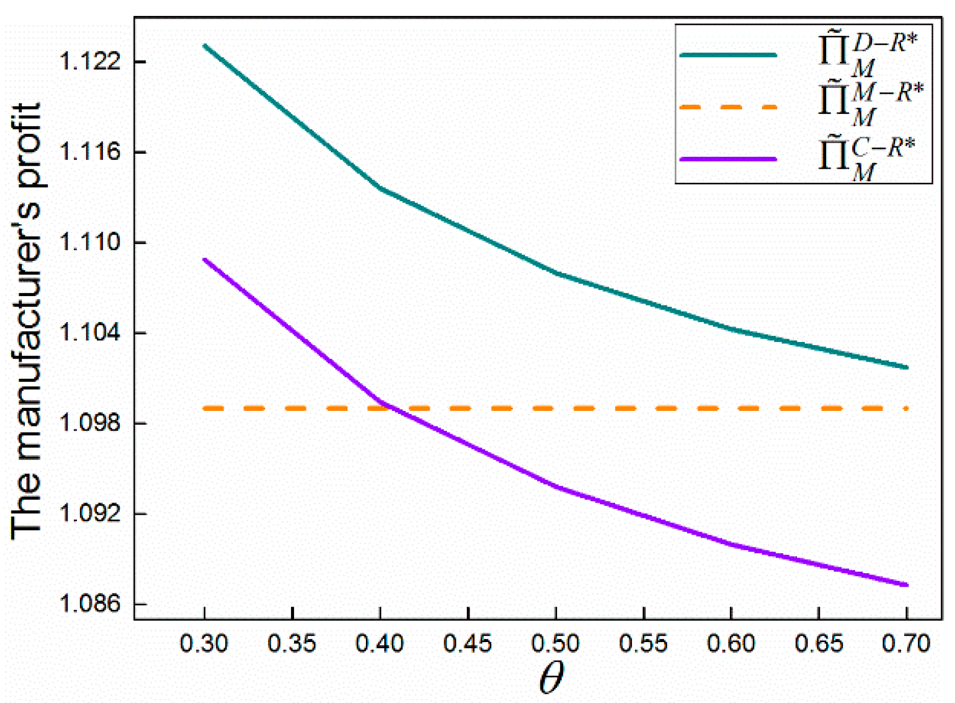
Then we turn to consider the manufacturer’s profit in the case of no disruption. Figure 6 indicates that the manufacturer can obtain more profits in dual-recycling channel than that in single-recycling channels regardless of the value of and has a negative impact on the manufacturer’s profit in both dual-recycling and online-recycling channels. In the dual-recycling channel, the manufacturer and the collector concurrently undertake collecting activities and the manufacturer’s profit will decrease with the increase of due to the intense competition between the manufacturer and the collector. Additionally, comparing online-recycling and offline-recycling channels, the manufacturer prefers offline-recycling channel when consumers’ preference to online-recycling is relatively low. If is relatively large, the manufacturer’s profit will be improved due to the lower handling cost of online-recycling channel.
Figure 7 demonstrates that has a negative impact on the quantity of remanufactured products. This phenomenon is caused by the increased remanufacturing cost. In the region of , the quantity of remanufactured products is the smallest when experiences sufficiently large positive disruption. While in the region of , the largest quantity of remanufactured products can be achieved when the negative disruption of is large enough. Notice that when the manufacturer acts as the channel leader, he would adjust the acquisition price and transfer price to maximize his own profits. Therefore, when the cost of new products is sufficiently small (i.e., ) and the remanufacturing cost is large enough, the manufacturer would produce more new products by decreasing the acquisition price and the transfer price. On the contrary, more used products will be collected and remanufactured due to a higher production cost of new products and a lower remanufacturing cost.
It is also found that, more products will be collected and remanufactured in dual-recycling channel than that in single-recycling channel and the quantity of remanufactured products in online-recycling channel is larger than that in offline-recycling channel. This finding comes from the fact that, the manufacturer and the collector have to set a higher acquisition price to recycle used products when facing recycling competition in dual-recycling channel. Regarding the quantity of remanufactured products, online-recycling channel dominates offline-recycling channel due to relatively large consumers’ preference to online-recycling channel (i.e., ). Moreover, no matter what the disruptions of and , the manufacturer always produces more remanufactured products in the dual-recycling channel than that in single-recycling channels.
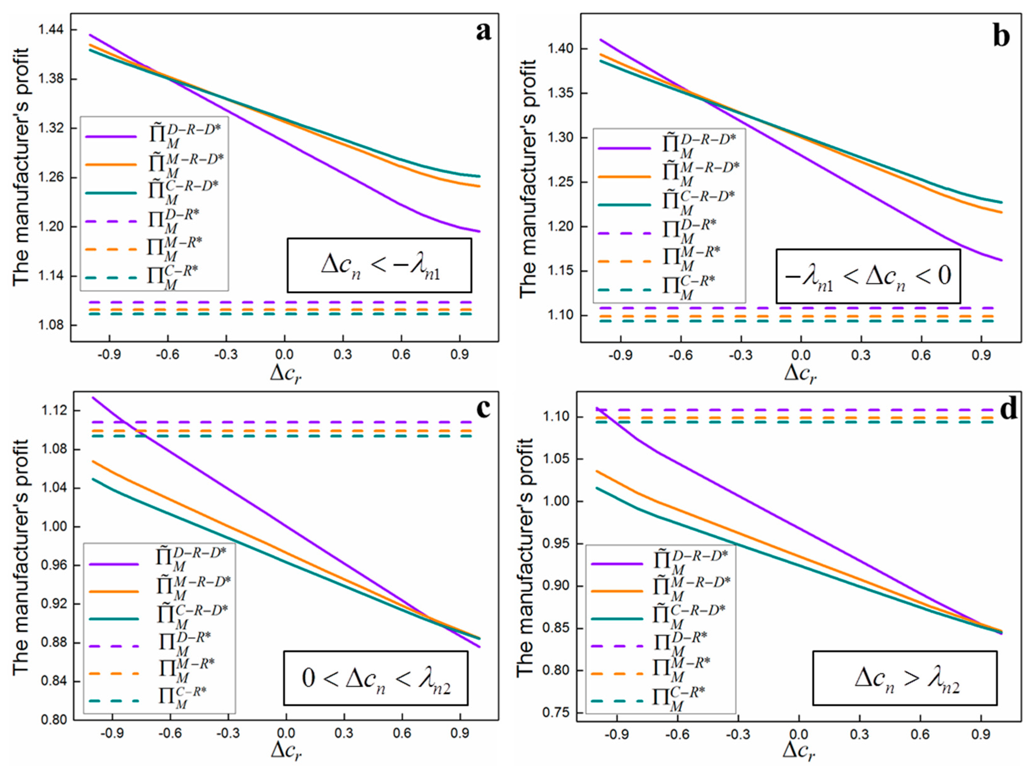
Subsequently, Figure 8 examines the impact of on the manufacturer’s profit in four regions of . Since the remanufacturing cost will be increased with the increase of in the same disruption of and the larger is, the smaller profit the manufacturer can achieve. Moreover, when the positive disruptions of and are sufficiently large, the manufacturer’s profit is the largest, while the manufacturer’s profit is the smallest when and experiences sufficiently large positive disruption. This can be explained that, when holds and is small enough, the manufacturer can earn more profits by producing both new and remanufactured products due to the lower production costs, while the manufacturer’s profit will decrease with the increase of and .
It can also be observed that, when experiences negative disruption, the manufacturer can obtain more profits in dual-recycling channel if the negative disruption of is large enough and otherwise single-recycling channel dominates dual-recycling channel. While if the disruption of is positive, as compared to single-recycling channels, the dual-recycling channel can bring more profits for the manufacturer. To be specific, in the regions of and , the manufacturer and the collector will increase the acquisition prices in dual-recycling channel when facing recycling competition and then more used products will be collected and remanufactured. When the negative disruption of is relatively large, the manufacturer can obtain more remanufacturing profits in dual-recycling channel due to a larger collection quantity of used products and a lower remanufacturing cost. While if experiences relatively small negative or positive disruption, the manufacturer prefers to produce more new products. Hence, a larger quantity of remanufactured products will result in a smaller profit for the manufacturer. On the other hand, if the cost of new products is relatively large (i.e., and ), the manufacturer would benefit from the larger quantity of remanufactured products.
7. Conclusions
This paper examines three recycling channels in the presence of cost disruptions of new and remanufactured products, namely online-recycling, offline-recycling and online-offline recycling. We analyze and compare the equilibrium strategies of each recycling channel with respect to cost disruptions and explore how consumers’ preferences to online-recycling channel affect the manufacturer’s collection and production strategies.
This research yields the following results. Firstly, in each recycling channel, the collection quantity of used products can be increased with the negative cost disruption of remanufactured products due to more cost savings from remanufacturing. The cost disruption of new products is conducive to improving the quantity of remanufactured products, because the manufacturer has no incentive to fabricate new products and accordingly produce more remanufactured products. Secondly, the manufacturer’s profit is increasing with the cost decrease of both new and remanufactured products. Since the manufacturer and the collector have to lift the acquisition prices to collect more used products when facing recycling competition in the dual-recycling channel, the manufacturer’s profit in dual-recycling channel is larger than that in single-recycling channels when the cost disruption of new products is positive. The case also holds when cost disruption of new products is negative and the remanufacturing cost faces sufficiently large negative disruption. Furthermore, comparing online-recycling and offline-recycling channels, if cost disruption of new products is positive, the online-recycling channel dominates offline-recycling channel when consumers’ preference to online-recycling channel is relatively high. In this case, the manufacturer can benefit from producing more remanufactured products. If new products experience negative cost disruption, the manufacturer would produce more new products and less remanufactured products. Therefore, the manufacturer prefers online-recycling channel if consumers’ preference to online-recycling is relatively high and otherwise he will subcontract offline-recycling channel to the collector. These results offer insights for understanding the relationship between the collection quantity and different disruption cases. Our results also provide managerial insights to help managers and decision-makers choose the most effective recycling strategies when facing disruption risks and to coordinate manufacturing and remanufacturing operations in their production processes to effectively mitigate disruption risks.
There are some limitations of this research should be pointed out. The price of remanufactured products is currently assumed to be same with new products, whereas in reality, the price of remanufactured products is often lower than that of new products. Additionally, the demand function is linear and fairly simple. It would be more interesting to adopt a non-linear demand function. There will be more implications about disruption risk in a dual-recycling channel CLSC.
Acknowledgments
This research is supported partially by the Humanities and Social Sciences Research Project of Education Department, Hubei province, China (16Y191); and Major Program of National Social Science Foundation of China (11&ZD165).
Author Contributions
Yanting Huang wrote the manuscript and participated in all phases. Zongjun Wang guided the research, discussed the results and commented on the manuscript at all stages. Both authors have read and approved the final manuscript.
Conflicts of Interest
The authors declare no conflict of interest.
Appendix A
Proof of Proposition 1.
Taking the second-order partial derivatives of with respect to and , we have the Hessian matrix
We can find that, is joint concave in and . Taking the first-order partial derivatives of with respect to and and letting the derivatives be zero, we have
□
Proof of Proposition 2.
We assume that and . Taking the second-order partial derivatives of with respect to and , we have the Hessian matrix
Since and , is concave in and . And other cases of and are similar. □
Proof of Proposition 3.
The second-order derivatives of with respect to is . Thus, is concave in .
And the optimal price strategy can be solved as follows:
Taking the second-order partial derivatives of with respect to and , we have the Hessian matrix
Therefore, is joint concave in and . The first-order partial derivatives of with respect to and can be given by
□
Proof of Proposition 4.
Taking the second-order derivative of with respect to , we can acquire . Hence, is concave in .
The optimal price strategy can be solved as follows:
Afterward, assume that and . Taking the second-order partial derivatives of with respect to and , we have the Hessian matrix
Therefore, is jointly concave in and .
And other cases of and are similar. □
Proof of Proposition 5.
Taking the second-order derivative of with respect to , we can attain . Thus, is concave in . And the optimal price strategy can be solved as follows:
Taking the second-order partial derivatives of with respect to , and , we have the Hessian matrix
We find that, is concave in , and . Taking the first-order partial derivatives of with respect to , and , we can obtain
□
Proof of Proposition 6.
Taking the second-order derivative of with respect to , we can obtain . Thus, is concave in . And taking the first-order derivative of , we have
Then we consider that and . Taking the second-order partial derivatives of with respect to , and , we have the Hessian matrix
Since and , is concave in , and .
And other cases of and are similar. □
Proof of Lemma 1.
In Model M-R-D, for the case of , since in case 4 and if holds, then we can get .
Subsequently, we can obtain
Since , then we can attain .
The proofs of the relationships of other prices and quantities are analogous. □
Proofs of Lemmas 2, 3 and 4.
The proofs of Lemmas 2, 3 and 4 are similar to the proof of Lemma 1. □
Proof of Lemma 5.
In Model C-R-D, for the region of , to prove , we examine that
After simplification, this reduces to showing that .
Meanwhile, as is satisfied in case 3 when holds, we can get that .
Similarly, and . Hence, we can get .
And the proofs of the relationships of other prices, quantities and profit are analogous. □
Proofs of Lemmas 6, 7 and 8.
The proofs of Lemmas 6, 7 and 8 are similar to the proof of Lemma 1. □
Proof of Lemma 9.
In Model D-R-D, we can get in the region of .
To prove , we have to show that
Similarly, we can get and . Thus, .
The proofs of the relationships of prices and profit are analogous. □
Proofs of Lemmas 10, 11 and 12.
The proofs of Lemmas 10, 11 and 12 are similar to the proof of Lemma 9.
Proof of Corollary 1.
To compare and in case 4, we have to show that
Therefore, as holds in case 4, we can get , when .
The proofs of the relationships of the selling prices and market demand in three recycling channels are analogous. □
Proof of Corollary 2.
In case 6, as and .
Therefore, to prove , we examine that
Moreover, as holds in case 6 and , we can get that .
Similarly, we can prove the relationship of the acquisition prices and transfer prices in online-recycling and dual-recycling channels when facing different disruption cases. □
Proof of Corollary 3.
To prove in case 1, we can obtain that
Then we can attain in case 1.
Similarly, we can get in other disruption cases. □
The proofs of the relationships of the acquisition prices in offline-recycling and dual-recycling channels are analogous.

Table A1.
The optimal selling price and demand in Model M-R-D.
| — — | , |
|---|---|
| case 1, 2 and 3 | |
| case 4 | |
| case 5 | |
| case 6 | |
| case 7, 8 and 9 |
Table A2.
The acquisition price and quantity in Model M-R-D.
| — — | , |
|---|---|
| case 1 | |
| case 2, 5 and 8 | , |
| case 3 | |
| case 4 | |
| case 6 | |
| case 7 | |
| case 9 |
Table A3.
The optimal manufacturer’s profit in Model M-R-D.
| Case | |
|---|---|
| 1 | |
| 2 | |
| 3 | |
| 4 | |
| 5 | |
| 6 | |
| 7 | |
| 8 | |
| 9 |
Table A4.
The optimal selling price and demand in Model C-R-D.
| — — | , |
|---|---|
| case 1, 2 and 3 | |
| case 4 | |
| case 5 | |
| case 6 | |
| case 7, 8 and 9 |
Table A5.
The prices, quantity and collector’s profit in Model C-R-D.
| — — | , , , |
|---|---|
| case 1 | |
| case 2, 5 and 8 | |
| case 3 | . |
| case 4 | |
| case 6 | |
| case 7 | |
| case 9 | |
Table A6.
The optimal manufacturer’s profit in Model C-R-D.
| Case | |
|---|---|
| 1 | |
| 2 | |
| 3 | |
| 4 | |
| 5 | |
| 6 | |
| 7 | |
| 8 | |
| 9 |
Table A7.
The optimal selling price and demand in Model D-R-D.
| — — | , |
|---|---|
| case 1, 2 and 3 | |
| case 4 | |
| case 5 | |
| case 6 | |
| case 7, 8 and 9 |
Table A8.
The prices, quantity and collector’s profit in Model D-R-D.
| Case | , , , , |
|---|---|
| 1 | |
| 2, 5, 8 | |
| 3 | |
| 4 | |
| 6 | |
| 7 | |
| 9 | |
Table A9.
The optimal manufacturer’s profit in Model D-R-D.
| Case | |
|---|---|
| 1 | |
| 2 | |
| 3 | |
| 4 | |
| 5 | |
| 6 | |
| 7 | |
| 8 | |
| 9 |
References
- Gaur, J.; Amini, M.; Rao, A.K. Closed-loop supply chain configuration for new and reconditioned products: An integrated optimization model. Omega 2017, 66, 212–223. [Google Scholar] [CrossRef]
- Atasu, A.; Souza, G.C. How Does Product Recovery Affect Quality Choice? Prod. Oper. Manag. 2013, 22, 991–1010. [Google Scholar] [CrossRef]
- Polotski, V.; Kenne, J.-P.; Gharbi, A. Production and setup policy optimization for hybrid manufacturing–remanufacturing systems. Int. J. Prod. Econ. 2017, 183, 322–333. [Google Scholar] [CrossRef]
- Esenduran, G.; Kemahlıoğlu-Ziya, E.; Swaminathan, J.M. Impact of Take-Back Regulation on the Remanufacturing Industry. Prod. Oper. Manag. 2017, 26, 924–944. [Google Scholar] [CrossRef]
- Ferrer, G.; Swaminathan, J.M. Managing New and Remanufactured Products. Manag. Sci. 2006, 52, 15–26. [Google Scholar] [CrossRef] [Green Version]
- Kumar, A.; Chinnam, R.B.; Murat, A. Hazard rate models for core return modeling in auto parts remanufacturing. Int. J. Prod. Econ. 2017, 183, 354–361. [Google Scholar] [CrossRef]
- Guide Jr, V.D.R.; Van Wassenhove, L.N. OR FORUM-the evolution of closed-loop supply chain research. Oper. Res. 2009, 57, 10–18. [Google Scholar] [CrossRef]
- Jia, J.; Xu, S.H.; Guide, V.D.R. Addressing Supply-Demand Imbalance: Designing Efficient Remanufacturing Strategies. Prod. Oper. Manag. 2016, 25, 1958–1967. [Google Scholar] [CrossRef]
- Subramanian, R.; Ferguson, M.E.; Beril Toktay, L. Remanufacturing and the Component Commonality Decision. Prod. Oper. Manag. 2013, 22, 36–53. [Google Scholar] [CrossRef]
- Zhou, L.; Naim, M.M.; Disney, S.M. The impact of product returns and remanufacturing uncertainties on the dynamic performance of a multi-echelon closed-loop supply chain. Int. J. Prod. Econ. 2017, 183, 487–502. [Google Scholar] [CrossRef]
- Feng, L.; Govindan, K.; Li, C. Strategic planning: Design and coordination for dual-recycling channel reverse supply chain considering consumer behavior. Eur. J. Oper. Res. 2017, 260, 601–612. [Google Scholar] [CrossRef]
- Ma, Z.-J.; Nian, Z.; Ying, D.; Shu, H. Managing channel profits of different cooperative models in closed-loop supply chains. Omega 2016, 59, 251–262. [Google Scholar]
- Xiao, T.; Qi, X.; Yu, G. Coordination of supply chain after demand disruptions when retailers compete. Int. J. Prod. Econ. 2007, 109, 162–179. [Google Scholar] [CrossRef]
- Li, Y.; Zhen, X.; Qi, X.; Cai, G. Penalty and financial assistance in a supply chain with supply disruption. Omega 2016, 61, 167–181. [Google Scholar] [CrossRef]
- Paul, S.K.; Sarker, R.; Essam, D. A quantitative model for disruption mitigation in a supply chain. Eur. J. Oper. Res. 2017, 257, 881–895. [Google Scholar] [CrossRef]
- Park, Y.; Hong, P.; Roh, J.J. Supply chain lessons from the catastrophic natural disaster in Japan. Bus. Horiz. 2013, 56, 75–85. [Google Scholar] [CrossRef]
- Genc, T.S.; De Giovanni, P. Trade-in and save: A two-period closed-loop supply chain game with price and technology dependent returns. Int. J. Prod. Econ. 2017, 183, 514–527. [Google Scholar] [CrossRef]
- He, Y. Acquisition pricing and remanufacturing decisions in a closed-loop supply chain. Int. J. Prod. Econ. 2015, 163, 48–60. [Google Scholar] [CrossRef]
- Xiong, Y.; Li, G.; Zhou, Y.; Fernandes, K.; Harrison, R.; Xiong, Z. Dynamic pricing models for used products in remanufacturing with lost-sales and uncertain quality. Int. J. Prod. Econ. 2014, 147, 678–688. [Google Scholar] [CrossRef]
- Li, X.; Li, Y.; Cai, X. Remanufacturing and pricing decisions with random yield and random demand. Comput. Oper. Res. 2015, 54, 195–203. [Google Scholar] [CrossRef]
- Han, X.; Wu, H.; Yang, Q.; Shang, J. Reverse channel selection under remanufacturing risks: Balancing profitability and robustness. Int. J. Prod. Econ. 2016, 182, 63–72. [Google Scholar] [CrossRef]
- Savaskan, R.C.; Bhattacharya, S.; Van Wassenhove, L.N. Closed-Loop Supply Chain Models with Product Remanufacturing. Manag. Sci. 2004, 50, 239–252. [Google Scholar] [CrossRef]
- Choi, T.-M.; Li, Y.; Xu, L. Channel leadership, performance and coordination in closed loop supply chains. Int. J. Prod. Econ. 2013, 146, 371–380. [Google Scholar] [CrossRef]
- Atasu, A.; Toktay, L.B.; Van Wassenhove, L.N. How Collection Cost Structure Drives a Manufacturer’s Reverse Channel Choice. Prod. Oper. Manag. 2013, 22, 1089–1102. [Google Scholar] [CrossRef]
- Mutha, A.; Bansal, S.; Guide, V.D.R. Managing Demand Uncertainty through Core Acquisition in Remanufacturing. Prod. Oper. Manag. 2016, 25, 1449–1464. [Google Scholar] [CrossRef]
- Savaskan, R.C.; Van Wassenhove, L.N. Reverse Channel Design: The Case of Competing Retailers. Manag. Sci. 2006, 52, 1–14. [Google Scholar] [CrossRef]
- Huang, M.; Song, M.; Lee, L.H.; Ching, W.K. Analysis for strategy of closed-loop supply chain with dual recycling channel. Int. J. Prod. Econ. 2013, 144, 510–520. [Google Scholar] [CrossRef]
- Hong, X.; Wang, Z.; Wang, D.; Zhang, H. Decision models of closed-loop supply chain with remanufacturing under hybrid dual-channel collection. Int. J. Adv. Manuf. Technol. 2013, 68, 1851–1865. [Google Scholar] [CrossRef]
- Yi, P.; Huang, M.; Guo, L.; Shi, T. Dual recycling channel decision in retailer oriented closed-loop supply chain for construction machinery remanufacturing. J. Clean. Prod. 2016, 137, 1393–1405. [Google Scholar] [CrossRef]
- Yu, H.; Zeng, A.Z.; Zhao, L. Single or dual sourcing: Decision-making in the presence of supply chain disruption risks. Omega 2009, 37, 788–800. [Google Scholar] [CrossRef]
- Tomlin, B. On the Value of Mitigation and Contingency Strategies for Managing Supply Chain Disruption Risks. Manag. Sci. 2006, 52, 639–657. [Google Scholar] [CrossRef]
- Xiao, T.; Qi, X. Price competition, cost and demand disruptions and coordination of a supply chain with one manufacturer and two competing retailers. Omega 2008, 36, 741–753. [Google Scholar] [CrossRef]
- Zhang, W.-G.; Fu, J.; Li, H.; Xu, W. Coordination of supply chain with a revenue-sharing contract under demand disruptions when retailers compete. Int. J. Prod. Econ. 2012, 138, 68–75. [Google Scholar] [CrossRef]
- Sawik, T. Joint supplier selection and scheduling of customer orders under disruption risks: Single vs. dual sourcing. Omega 2014, 43, 83–95. [Google Scholar] [CrossRef]
- Giri, B.C.; Sarker, B.R. Improving performance by coordinating a supply chain with third party logistics outsourcing under production disruption. Comput. Ind. Eng. 2017, 103, 168–177. [Google Scholar] [CrossRef]
- Han, X.; Wu, H.; Yang, Q.; Shang, J. Collection channel and production decisions in a closed-loop supply chain with remanufacturing cost disruption. Int. J. Prod. Res. 2016, 55, 1147–1167. [Google Scholar] [CrossRef]
- Giri, B.C.; Sharma, S. Optimal production policy for a closed-loop hybrid system with uncertain demand and return under supply disruption. J. Clean. Prod. 2016, 112, 2015–2028. [Google Scholar] [CrossRef]
- De Giovanni, P.; Reddy, P.V.; Zaccour, G. Incentive strategies for an optimal recovery program in a closed-loop supply chain. Eur. J. Oper. Res. 2016, 249, 605–617. [Google Scholar] [CrossRef]
Figure 1.
Closed-loop supply Chain Models with Remanufacturing. (a) Model M-R; (b) Model M-R-D; (c) Model C-R; (d) Model C-R-D; (e) Model D-R; (f) Model D-R-D.
Figure 1.
Closed-loop supply Chain Models with Remanufacturing. (a) Model M-R; (b) Model M-R-D; (c) Model C-R; (d) Model C-R-D; (e) Model D-R; (f) Model D-R-D.
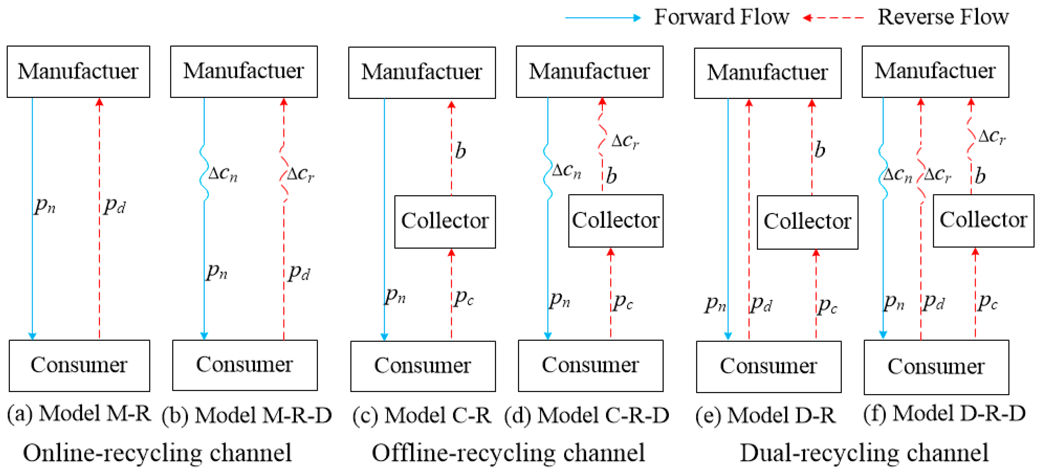
Figure 2.
The disruption cases in Model M-R-D in the case of (a) ; and (b) .
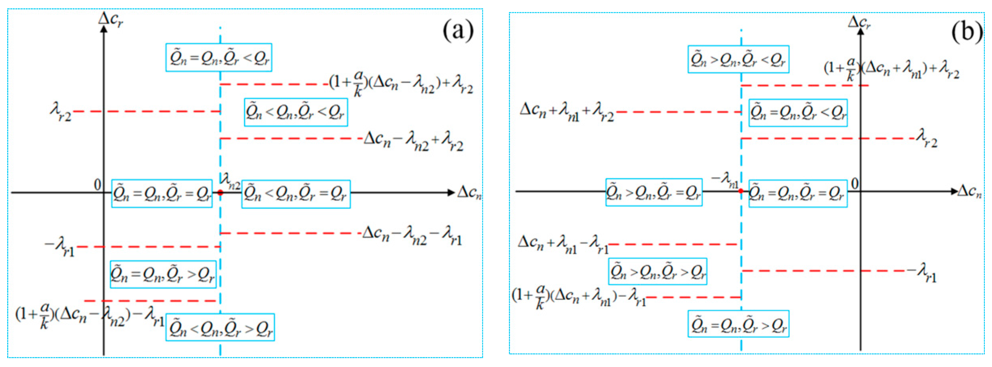
Figure 3.
The disruption cases in Model C-R-D in the case of (a) ; and (b) .
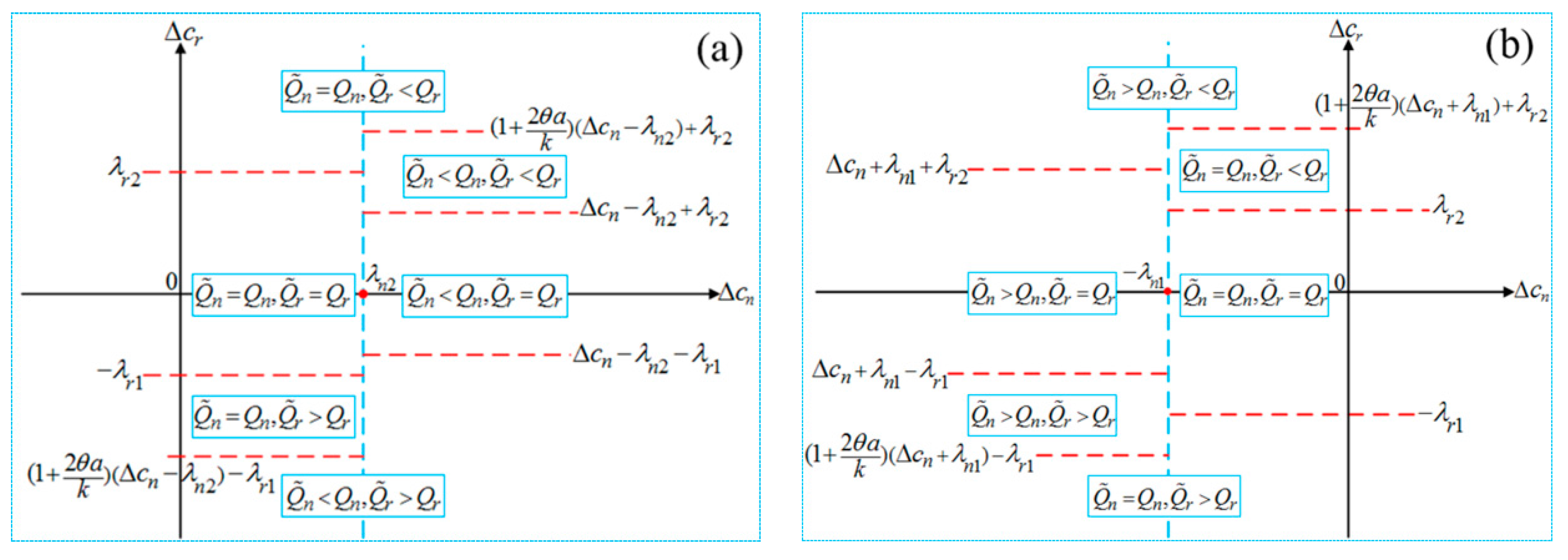
Figure 4.
The disruption cases in Model D-R-D in the case of (a) ; and (b) .
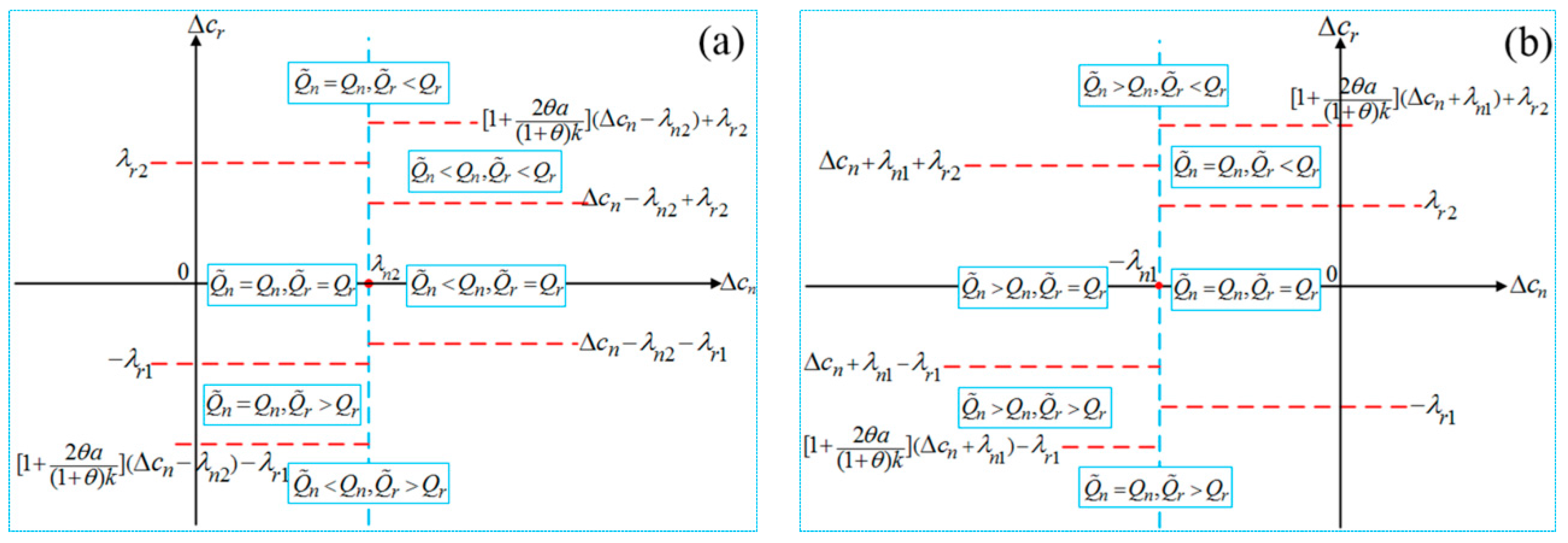
Figure 5.
The quantity of remanufactured products with different .
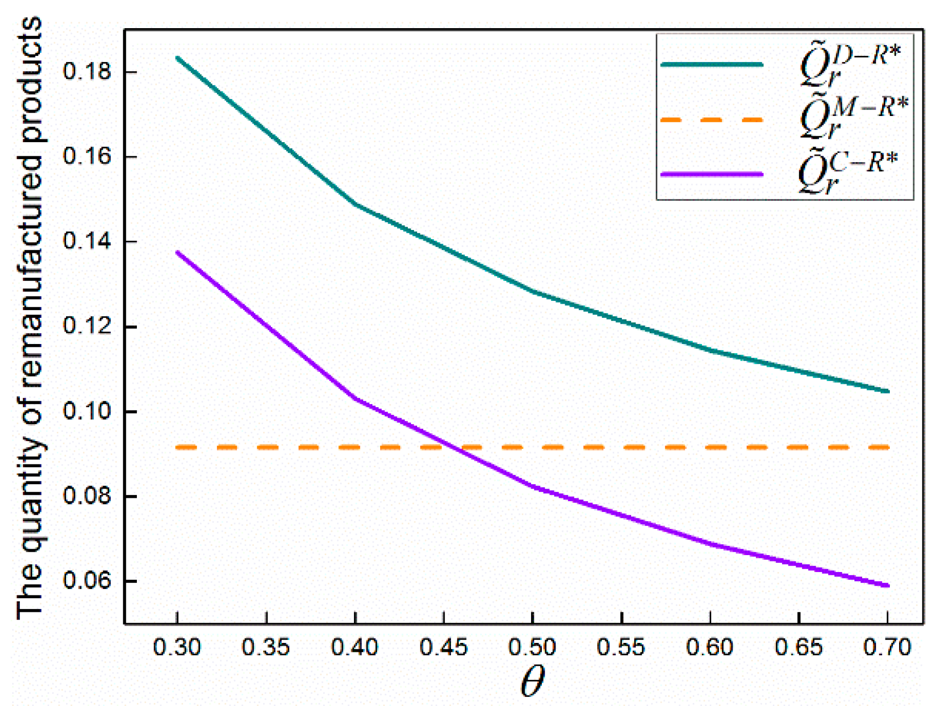
Figure 6.
The manufacturer’s profit with different .

Figure 7.
The quantity of remanufactured products with different in the case of (a) ; (b) ; (c) ; and (d) .
Figure 7.
The quantity of remanufactured products with different in the case of (a) ; (b) ; (c) ; and (d) .
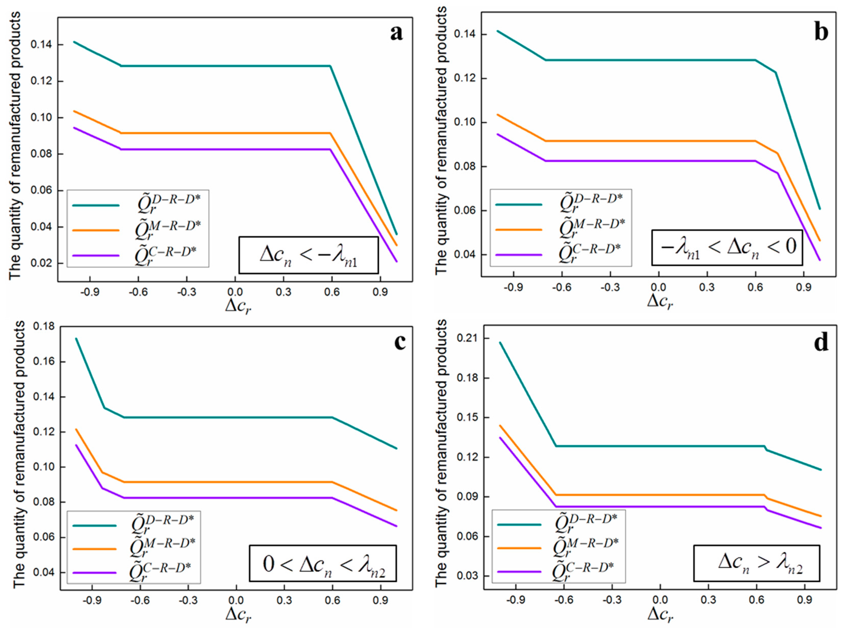
Figure 8.
The manufacturer’s profit with different in the case of (a) ; (b) ; (c) ; and (d) .

Table 1.
Parameters and definitions.
| Notation | Definition |
|---|---|
| The unit selling price | |
| The average unit cost of manufacturing new products by the manufacturer | |
| The average unit cost of remanufacturing returned products by the third party | |
| , | The unit acquisition prices of the manufacturer and the collector, respectively |
| The unit transfer price from the manufacturer to the collector | |
| The market demand function | |
| Sensitivity of consumers to the selling price | |
| The quantity of remanufactured products | |
| , | The collection quantity of used products under online-recycling and offline-recycling channels, respectively |
| Profit |
Table 2.
The disruption cases in Model M-R-D.
| , | , |
|---|---|
| , | case 1: |
| , | case 2: |
| (1) , (2) , | case 3: |
| (1) , (2) , (3) , | case 4: |
| , | case 5: , |
| (1) , ; (2) ,; (3) , ; | case 6: |
| (1) , (2) , | case 7: |
| , | case 8: |
| , | case 9: |
Table 3.
The relations of quantities in the cases of disruption and no disruption.
| — | vs. | vs. | — | vs. | vs. | — | vs. | vs. |
|---|---|---|---|---|---|---|---|---|
| Case 1 | > | > | Case 4 | = | > | Case 7 | < | > |
| Case 2 | > | = | Case 5 | = | = | Case 8 | < | = |
| Case 3 | > | < | Case 6 | = | < | Case 9 | < | < |
Table 4.
The disruption cases in Model C-R-D.
| , | , |
|---|---|
| , | case 1: |
| , | case 2: |
| (1) , (2) , | case 3: |
| (1) , (2) , (3) , | case 4: |
| , | case 5: , |
| (1) , (2) , (3) , | case 6: |
| (1) , (2) , | case 7: |
| , | case 8: |
| , | case 9: |
Table 5.
The disruption cases in Model D-R-D.
| , | , |
|---|---|
| , | case 1: |
| , | case 2: |
| (1) , (2) , | case 3: |
| (1) , (2) , (3) , | case 4: |
| , | case 5: , |
| (1) , (2) , (3) , | case 6: |
| (1) , (2) , | case 7: |
| , | case 8: |
| , | case 9: |
Table 6.
The relations of the optimal decisions in online-recycling channel with changing .
| Lemma 1 | Lemma 2 | Lemma 3 | Lemma 4 |
|---|---|---|---|
| If , | If , | If , | If , |
Table 7.
The relations of the optimal decisions in offline-recycling channel with changing .
| Lemma 5 | Lemma 6 | Lemma 7 | Lemma 8 |
|---|---|---|---|
| If , | If , | If , | If , |
Table 8.
The relations of the optimal decisions in dual-recycling channel with changing .
| Lemma 9 | Lemma 10 | Lemma 11 | Lemma 12 |
|---|---|---|---|
| If , | If , | If , | If , |
© 2017 by the authors. Licensee MDPI, Basel, Switzerland. This article is an open access article distributed under the terms and conditions of the Creative Commons Attribution (CC BY) license (http://creativecommons.org/licenses/by/4.0/).
Share and Cite
MDPI and ACS Style
Huang, Y.; Wang, Z. Dual-Recycling Channel Decision in a Closed-Loop Supply Chain with Cost Disruptions. Sustainability 2017, 9, 2004. https://doi.org/10.3390/su9112004
AMA Style
Huang Y, Wang Z. Dual-Recycling Channel Decision in a Closed-Loop Supply Chain with Cost Disruptions. Sustainability. 2017; 9(11):2004. https://doi.org/10.3390/su9112004
Chicago/Turabian StyleHuang, Yanting, and Zongjun Wang. 2017. "Dual-Recycling Channel Decision in a Closed-Loop Supply Chain with Cost Disruptions" Sustainability 9, no. 11: 2004. https://doi.org/10.3390/su9112004
Note that from the first issue of 2016, this journal uses article numbers instead of page numbers. See further details here.