Article

Life Cycle Assessment of Two Vineyards after the Application of Precision Viticulture Techniques: A Case Study

by
Athanasios T. Balafoutis
1,2,*,
Stefanos Koundouras
3,
Evangelos Anastasiou
1,
Spyros Fountas
1 and
Konstantinos Arvanitis
1
1
Department of Natural Resources Management & Agricultural Engineering, Agricultural University of Athens, Iera Odos 75, 11855 Athens, Greece
2
Institute of Bioeconomy & Agrotechnology, Centre of Research & Technology Hellas, Dimitriados 95 & Pavlou Mela, 38333 Volos, Greece
3
Laboratory of Viticulture, School of Agriculture, Aristotle University of Thessaloniki, 54124 Thessaloniki, Greece
*
Author to whom correspondence should be addressed.
Sustainability 2017, 9(11), 1997; https://doi.org/10.3390/su9111997
Submission received: 12 August 2017 / Revised: 28 August 2017 / Accepted: 6 October 2017 / Published: 1 November 2017

Abstract

:
Precision viticulture is the application of site-specific techniques to vineyard production to improve grape quality and yield and minimize the negative effects on the environment. While there are various studies on the inherent spatial and temporal variability of vineyards, the assessment of the environmental impact of variable rate applications has attracted limited attention. In this study, two vineyards planted with different grapevine cultivars (Sauvignon Blanc and Syrah) were examined for four consecutive growing seasons (2013–2016). The first year, the two vineyards were only studied in terms of soil properties and crop characteristics, which resulted in the delineation of two distinct management zones for each field. For the following three years, variable rate nutrient application was applied to each management zone based on leaf canopy reflectance, where variable rate irrigation was based on soil moisture sensors, meteorological data, evapotranspiration calculation, and leaf canopy reflectance. Life cycle assessment was carried out to identify the effect of variable rate applications on vineyard agro-ecosystems. The results of variable rate nutrients and water application in the selected management zones as an average value of three growing seasons were compared to the conventional practice. It was found that the reduction of product carbon footprint (PCF) of grapes in Sauvignon Blanc between the two periods was 25% in total. Fertilizer production and distribution (direct) and application (indirect) was the most important sector of greenhouse gas (GHG) emissions reduction, accounting for 17.2%, and the within-farm energy use was the second ranked sector with 8.8% (crop residue management increase GHG emissions by 1.1%, while 0.1% GHG reduction is obtained by pesticide use). For the Syrah vineyard, where the production was less intensive, precision viticulture led to a PCF reduction of 28.3% compared to conventional production. Fertilizers contributed to this decrease by 27.6%, while within-farm energy use had an impact of 2.2% that was positive even though irrigation was increased, due to yield rise. Our results suggest that nutrient status management offers the greatest potential for reducing GHG emissions in both vineyard types. Variable rate irrigation also showed differences in comparison to conventional treatment, but to a lesser degree than variable rate fertilization. This difference between conventional practices and precision viticulture is noteworthy, and shows the potential of precision techniques to reduce the effect of viticulture on GHG emissions.

1. Introduction

Agricultural productivity has seen a significant increase since the mid-twentieth century, due to the existence of new technologies in agriculture [1]. However, there are numerous environmental impacts as a result of intensive agricultural practices and agricultural mechanisation. These include soil erosion and loss of soil organic matter [2,3,4,5]; excessive nitrogen use [6,7]; reduction of water reserves above ground and in the aquifer [8]; and excessive pesticide use that causes numerous environmental problems (eutrophication, ecotoxicity, soil degradation and acidification) [9]. In addition, human exposure to low-dose pesticide mixtures by interacting with pesticide-mistreated products produces a long-lasting negative health impact [10]. The agricultural sector significantly affects climate change, accounting for nearly 13.5% of the total global anthropogenic greenhouse gas (GHG) production [11]. The major GHGs produced in this sector are methane (CH4), nitrous oxide (N2O), and carbon dioxide (CO2). The main agricultural source of CH4 is the anaerobic decomposition of organic matter during enteric fermentation, manure management, and paddy rice cultivation, while N2O is mainly synthesised from the microbial transformation of soil nitrogen during the application of manure and synthetic fertilisers in agricultural land and via urine and dung deposited by grazing animals. Finally, CO2 arises directly from energy use in the farm (fuels, electricity) and from changes in above- and below-ground carbon stocks induced by land use and land use change [12].
The United Nations Framework Convention on Climate Change (UNFCC) and the Intergovernmental Panel on Climate Change (IPCC) have developed concrete methodologies for GHG calculations [13], where life cycle assessment (LCA) is the most well-known method, which attempts to cover all attributes or aspects of natural environment, human health, and resources [14,15]. LCA is a method used to measure the overall environmental impact caused by the product or process under study from the very beginning to the end [16,17]. In the primary sector and especially in agriculture, some of the principles arising from LCA modelling are the environmental, technological, and socioeconomic factors that influence the existence of numerous inconsistencies from the “average” farm practices. Machinery production and maintenance has an impact on GHG emissions and energy consumption, while irrigation, fertilization, and nutrient management (especially nitrogen) are important variables in the environmental performance index of crop production [18].
Viticulture is a very important agricultural sector for either wine (principally) or table grape production. Christ and Burritt (2013) pointed out that the critical environmental impacts of wine production are the water, land, and energy use, the management of organic and inorganic solid waste streams, the generation of GHG emissions, and the use of chemicals [19]. As viticulture contributes about 12 MT of CO2eq per year to the product carbon footprint (PCF) of wine [20,21,22], wine-producing stakeholders are very much interested in increasing the environmental sustainability of the vineyard system. The sources of GHG emissions in viticulture come from fertilizer and pesticide production and transportation, soil emissions, crop residue management, energy use for irrigation, pruning, tillage, fertilizer and pesticide application, compiling the total PCF of wine grapes [23]. Bosco et al. (2011) concluded that the planting of vine trees and trellis systems contributed significantly to the GHG emissions when the system starts from scratch. Additionally, intensive production practices tend to produce larger amounts of GHG [22,24,25]. Mitigation strategies for GHG emissions from viticulture production can be identified by inventorying and reporting the PCF through LCA, taking into consideration emissions, material, and energy inputs [24,26,27]. Previous research has established that organic fertilization leads to substantial savings in GHG emissions [28,29,30]. Another key point to mitigate viticulture GHG emissions is the use of cultivars already adapted to local conditions that require less inputs [24,31] and the reduction of energy requirements in a vineyard that are affected by size, topography, degree of mechanisation, and end-use of the grapes [31,32]. Currently, viticulture is gradually shifting to more sustainable production patterns [33], with an increase of 230% of organic vineyards in Europe between 2007 and 2011 [34]. A number of studies have been carried out comparing different types of viticulture techniques (i.e., organic, biodynamic, and conventional) in order to assess their environmental impacts through the life assessment approach [25,34,35].
Vázquez-Rowe et al. (2012) [36] implemented a combined LCA with data envelopment analysis (DEA), which is a suitable tool for assessing multiple input/output data in agrifood systems to determine the level of operational efficiency for grape production. They analysed 40 vineyards and found average reductions in input consumption levels ranging from 8% to 30%, average environmental gains from 28% to 39% for a set of six impact categories, and 10% average increase in economic benefits for inefficient units turning efficient. Rugani et al. (2013) [25] carried out an extensive review on product carbon footprint (PCF) analyses of wine production, and observed methodological and conceptual limits and challenges behind wine PCF, but pointed out that indicating wine PCF may provide large benefits both to winemakers and consumers. Villanueva-Rey et al. (2014) [35] performed a comparative LCA in biodynamic and conventional viticulture activities in North-western Spain and concluded that biodynamic production implies the lowest environmental burdens, while the highest environmental impacts were linked to conventional agricultural practices, mainly due to an 80% decrease in diesel inputs related to lower pesticide and fertilisers application and the introduction of manual work rather than mechanised activities in the vineyards. Rouault et al. (2016) [34] compared organic and integrated viticultural technical management routes using LCA techniques, with the result that the studied organic route had higher impact scores than the integrated for all the chosen impact categories except eutrophication.
Venkat (2012) [37] compared GHG emissions for 12 crop products, including wine grapes grown in organic and conventional farming systems. Results showed that converting to organic production may offer significant GHG reduction by increasing the soil organic carbon stocks during the transition phase and that conventional systems could improve their environmental performance by adopting management practices that increase soil organic carbon stocks. Aguilera et al. (2015) [38] conducted research on a LCA of conventional and organic fruit tree orchards including vineyards in Spain, and concluded that machinery use in vineyards accounted for more than 60% of the total global warming potential. Litskas et al. (2017) [23] determined the PCF of indigenous and introduced grape cultivars through LCA in Cyprus. They concluded that fertilizers and field energy use were the major carbon sources for viticulture. The application of animal manure instead of synthetic fertilizers and the reduction of tillage frequency could potentially reduce the PCF by 40–67%. They also concluded that PCF is affected mostly by the harvest yield (3–8% potential PCF change) [21].
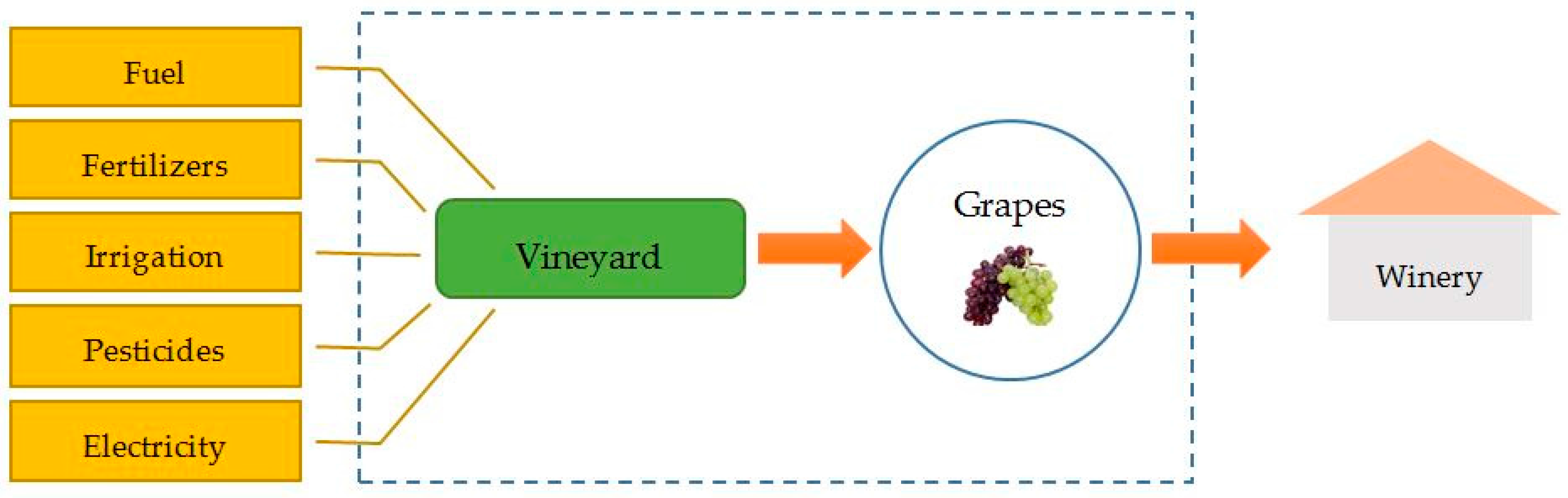
The environmental behaviour of viticultural systems could also be improved by the application of precision viticulture (PV) techniques. PV is a circular process which entails data collection, data analysis, decision-making about management, and evaluation of these decisions [39]. In this way, the advantages of the vineyard variability in favour of the producer are fully exploited and the application of agricultural inputs (fuel, fertilisers, pesticides, water) is minimised for the maximum yield and quality of produced grapes [40,
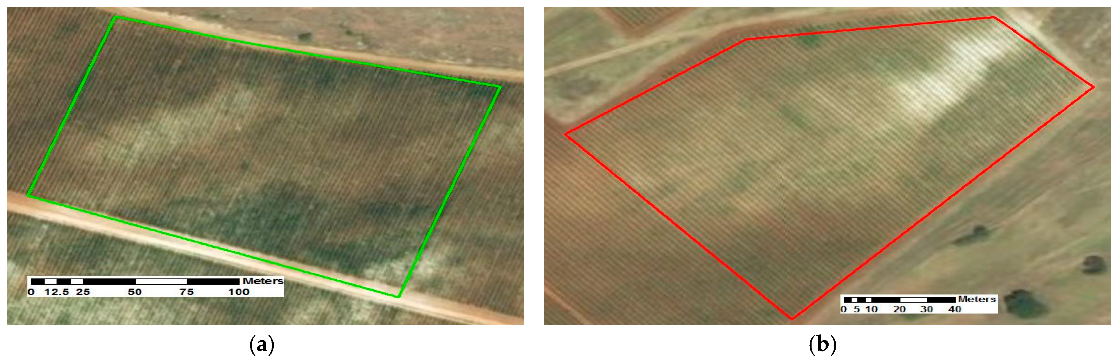
41]. However, the impact of PV on the environment and especially in GHG emissions has not received the attention deserved, with limited results in literature. Hence, in this study a comparative analysis between conventional and PV agricultural practices of two commercial vineyards planted with two different cultivars regarding GHG emissions was carried out in order to quantify in a deterministic basis the environmental benefits of PV in terms of GHG emissions. The structure of this work starts with the description of the vineyards’ input and output of conventional practices and continues with the methodology of delineating management zones that is accompanied with the inventory of PV practices. Subsequently, the methodology of LCA using the selected tool (Cool Farm Tool) is described and the results in product carbon footprint of both the conventional and PV vineyards is presented and discussed, ending with the final conclusions.

2. Materials and Methods

2.1. Selected Vineyards

The study was conducted in two commercial vineyards in Northern Greece in four vintages (2013 till 2016). The first was planted with Vitis vinifera L. cv. Sauvignon Blanc (41°5.5′ N, 23°55.8′ E, Drama, Greece) and the second with Vitis vinifera L. cv. Syrah (41°5.8′ N, 23°56.7′ E, Drama, Greece) at 2.4 and 1.7 ha, respectively (Figure 1).
Sauvignon Blanc (SB) vines were established on a sandy loam soil on a relatively steep slope in 2005, while Syrah (SY) vines were planted on a sandy clay loam with lower slope in 2006. Both cultivars were grafted onto 1103 Paulsen rootstock, trained to a bilateral cordon and spaced 1.2 × 2.2 m (3740 vines/ha). Both cultivation periods experienced similar weather conditions in terms of precipitation and average temperature during the growing season.
In order to measure the outputs of the reference year and follow their progress in the following years, the two vineyards were split into grid cells of 0.1 ha, as shown in Figure 2; 24 and 17 grid cells were delineated in SB and SY vineyards, respectively.

2.2. Conventional Practices

Conventional local management practices were applied to the two vineyard cultivars in the 2013 vintage, which stands as the reference to compare to the PV practices in the consecutive years (2014, 2015, and 2016). The agricultural practices, the number of actions of each practice, and the total quantities of inputs and outputs in both vineyards are shown in Table 1, presented per ha. Nutrient application was the same for both vineyards, feeding the soil with 597 kg/ha NH4NO3 (200 kg N/ha) and 250 kg/ha K2SO4 (120 kg K/ha) through the irrigation system (fertigation) combined with 30 t/ha of sheep manure spreading incorporated through soil tillage. The most important difference was that SB was irrigated ten times during the season receiving a total of 300 mm of water (30 mm per application), while SY was irrigated only four times with 20 mm doses, leading to higher yield, overall vigour, canopy size, and weed population for SB. Water was delivered by a drill with a pump of 60 m3/h using an electric motor of 75 kW and the final electricity use for water pumping was much higher (3750 kWh/ha) in SB than in SY, where it reached 1000 kWh/ha. Fertilizer and water application combination resulted in more vineyard operations (trimming, leaf plucking) in the SB vineyard to adjust the results of more vigorous vegetation and weed population (soil tillage and intra-row mowing), while SY was minimally managed. SB vineyard was also treated 11 times (spraying, dusting) with different pesticide types due to denser canopy being more prone to threats, while SY required 8 treatments. All these agricultural practices resulted in tractor fuel use in SB of 105.6 kg/ha and in SY 67.8 kg/ha.
Grape harvest was performed manually on 18 and 24 August 2013 for SB and SY, yielding 12.69 and 7.01 t/ha respectively. Winter pruning was also executed manually on February 2014, and it was weighted to be 3.66 t/ha in SB and 1.22 t/ha in SY, reflecting the difference in canopy volume and structure during the production season. To assist the following analysis of GHGs, yield and pruning were measured for each cell of the two vineyards. The pruned canes were shred and incorporated into the soil after light tillage.

2.3. Precision Viticulture Practices

In order to apply PV techniques in the above vineyards, the field was delineated into management zones. First, the boundaries of the vineyards were geo-referenced using GPS technology, and then time-stable zones were formed using soil electrical conductivity (ECa) mapping, assisted by elevation mapping using RTK-GPS (HiPer V, Topcon Co., Tokyo, Japan) [40]. ECa measurements were taken using an EM-38 probe (EM38 RT, Geonics LTD, Mississauga, ON, Canada), and the results are shown in Figure 3.
Elevation and slope data were acquired from SRTM satellite in Global Mapper 14 (Blue Marble Geographics, Hallowell, ME, USA) and are shown in Figure 4.
The delineated management zones were produced with Management Zone Analyst 1.0.1 (MZA) (University of Missouri, Columbia, MO, USA), and the maps were generated in ArcGIS 10.2.2 (ESRI, Redlands, CA, USA), as shown in Figure 5.
The surface of each management zone was equal for the SB vineyard (1.2 ha) and different in SY (0.7 and 1 ha, respectively). Based on the two delineated zones, all data for the agronomic (soil, vigour, yield) and meteorological parameters of the vineyards were used to calculate the proposed dosage for fertilization and irrigation for consecutive vintage. To alleviate year-to-year variation in the final results of the analysis, the same procedure was followed for the consecutive seasons (2015 and 2016) and an average value for the three years of PV application of both irrigation and fertilization dosages were used in the comparison analysis between conventional and PV practices.
Irrigation volumes per zone were estimated as a fraction of actual evapotranspiration (ETa) per management zone. ETa was calculated using ET estimated by the automatic weather station installed inside the vineyard and vigour measurements (Normalized Difference Vegetation Index—NDVI) at various vine developmental stages, according to the method developed by Groeneveld et al. (2007) [42]. The strategy was to maintain all vines within the vineyard at a similar water status of a light water deficit which is beneficial for vine balance and grape quality [43]. This was achieved by applying less water to high-vigour areas (25% of ETa) and more water to low-vigour areas (75% of ETa).
Assessment of vigour remains the best practical solution for the evaluation of vine nitrogen needs, in the absence of an accurate method of determining the amount of available nitrogen for the vine in the soil and perennial parts. Similarly to water application, to decrease vineyard variability, zones with lower vigour in the previous season received—at budburst—an increased amount of N (60–90 kg/ha) as ammonium nitrate, compared to more vigorous areas (30–60 kg/ha) [44]. Nitrogen fertilizer applications were also decided upon vigour assessment of the current season by NDVI measurements at veraison stage (Table 2). For potassium-variable fertilizer applications, the depletion model for annual applications was used (2–2.5 kg K removed per 1 t of grapes) to determine potassium sulphate doses per management zone [45]. Table 3 shows the inputs and outputs that were differentiated after PV practices in the period 2014–2016, while the rest of the practices remained the same as in conventional viticulture.
Fertilization dosage was separated for the two management zones for both vineyards, and each growing season received different quantities of NH4NO3 and K2SO4, as shown in Table 3. The average values of both fertilizer types in zone 1 of the SB vineyard were 363.2 kg/ha NH4NO3 and 123.7 kg/ha K2SO4, while in zone 2 they were 283.6 kg/ha NH4NO3 and 152.9 kg/ha K2SO4 (120 kg K/ha). In the SY vineyard, average fertilisation in zone 1 was 557.2 kg/ha NH4NO3 and 131.8 kg/ha K2SO4, and in zone 2 it was 288.6 kg/ha NH4NO3 and 155 kg/ha K2SO4. Finally, the reduction of the total fertilizer application of NH4NO3 in comparison to conventional practice was 45.8% in SB and 33.1% in SY, while K2SO4 was decreased in both cases (44.7% and 41.8% in SB and SY, respectively). It can be seen that nitrogen fertilization was significantly reduced using PV practices, as it was ascertained that there was an excess use of nitrogen that was not used by the vines. Regarding potassium application in both vineyards, it was found that there was a deficit of potassium that was reflected negatively in quality parameters, and therefore in 2014 high potassium quantities were applied to enrich soils, while the consecutive seasons (2015, 2016) followed the above-mentioned depletion model, translating into much lower K2SO4 application (Table 3). There was year-to-year fluctuation for both fertilizer types based on vigour, soil, and yield measurements, but this variation remained within acceptable limits (SB vineyard: CV = 5.1% and 4.3% for zones 1 and 2, respectively; SY vineyard: CV = 2.5% and 2.4% for zones 1 and 2, respectively), indicating that both vineyards after splitting them in zones showed stability in fertilization needs over growing seasons.
Management zones were irrigated differently during the three seasons of PV practices application, keeping the number of water applications the same as in the 2013 vintage. In the SB vineyard, irrigation dose was on average almost the same as in 2013 in zone 1 (293.3 mm in total), while it was reduced significantly in zone 2 (206.7 mm in total). In SY, zone 1 received 120 mm of total average irrigation and zone 2 was watered with 63.3 mm. The result was to apply on average 600 mm per annum in the SB vineyard, decreasing water use by 16.7% and increasing irrigation in the SY vineyard by 8.3% (application of 147.3 mm per annum).
As rainfall and temperature varied notably in the period of the experiment (Table 4), the irrigation regime fluctuated higher than fertilization (SB vineyard: CV = 8.5% and 12% for zones 1 and 2 respectively; SY vineyard: CV = 13.6% and 19.7% for zones 1 and 2 respectively) in order to supply vines with water when required.

2.4. Product Carbon Footprint (PCF)

The differences between the conventional viticulture practices and the PV techniques were evaluated in terms of GHG emissions and carbon balance using the Cool Farm Tool (www.coolfarmtool.org). The selection of this tool was based on Whittaker et al. (2013) [46], which compared this tool with ten other GHG calculators for either single crops or for whole farms (CALM, C-PLAN, CCalc, Organic Farmer Carbon calculator, Muntons barley calculator, Biograce calculator, RFA e RTFO Carbon Calculator, BEATv2, RSB Tool, HGCA Biofuel GHG Calculator) using multi-criteria decision-making methods, and it was concluded that the Cool Farm Tool was the highest-rated tool recommended for single crop assessments like the case study of this work.
The procedure followed by Cool Farm Tool is based on the principles of LCA under the framework of IPCC (2006) [47] for GHG calculation. The goal of this procedure was to measure the product carbon footprint (PCF) of grape production as a feedstock for wineries, and the functional unit selected was one tonne of grapes. Therefore, the PCF would be given as kg CO2eq/t of grapes. The analysis conducted in this work included all agricultural practices in both conventional and precision viticulture within the system boundary that was set to be the vineyard gate (Figure 6).
The parameters considered in the Cool Farm Tool for calculating the PCF of grapes are given in Table 5, excluding emissions arising from land use change (SB and SY vineyards were planted in 2005 and 2006, respectively) and tillage changes that remained the same in both seasons. All inputs and output calculations of this tool are analysed in detail in Hillier et al. (2011) [48]. The Cool Farm Tool requires data on harvested yield and marketable yield product, growing area, fertiliser applications in terms of type and rate, number of pesticide applications, energy and fuel use, and optionally transport in terms of mode, weight of product, and distance.

2.5. Statistical Analysis

In order to define whether PCF differences between conventional practices and each of the three consecutive PV vintages were statistically significant in both SB and SY vineyards, paired sample t-tests between the reference season (2013) and each of the PV seasons (2014, 2015, 2016) were executed. As a second step, Cochran’s Q-test was used to identify the proportion of PCF values in the PV seasons being lower (shown as 0) or higher (shown as 1) as compared to the reference season. The PCF values under analysis were extracted for each cell shown in Figure 2. All statistical analyses were conducted using SPSS 23 (IBM Corp., New York, NY, USA).

3. Results

3.1. Product Carbon Footprint of Sauvignon Blanc Vineyard

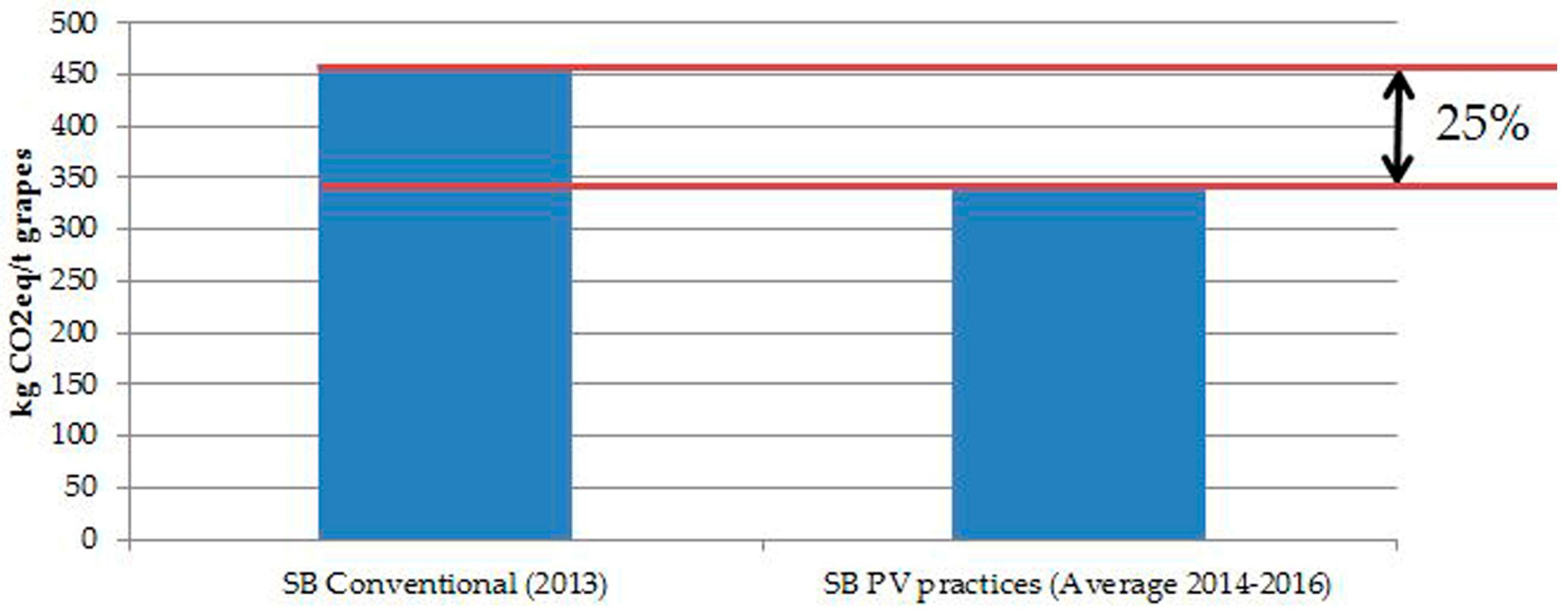
The PCF of the SB vineyard with conventional practices in the 2013 vintage reached 452.6 kg CO2/t grapes. After PV practices for three consecutive growing seasons, the average PCF was 339.3 kg CO2/t grapes, leading to a reduction of 113.3 kg CO2eq/t grapes (25%), as shown in Figure 7.
The paired sample t-tests showed that PCF values were lower for all consecutive years in comparison to 2013, with p < 0.05 statistical significance (95% confidence interval of the difference). As for the Q-tests, it was shown that the frequency of PCF values in the three consecutive seasons that were lower than the respective values in 2013 (shown as 0) was trending to significant over the three PV seasons (Table 6).
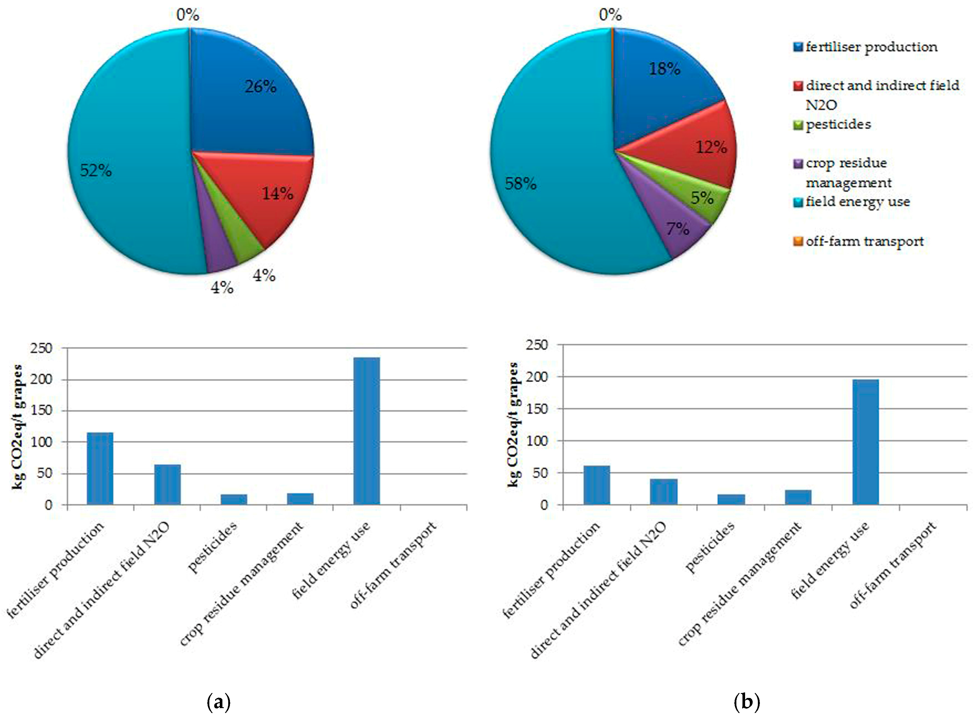
The distribution of emissions among the agricultural practices followed in both conventional viticulture of 2013 and PV as an average of three consecutive seasons using PV practices (2014–2016) are given in Figure 8. The most significant activity regarding GHG emissions was field energy, which combines fuel for tractor use and electricity for irrigation in both conventional and PV practices, counting for 235.1 and 195.2 kg CO2eq/t grapes, respectively (52% and 58% of the total GHG emissions). In 2013, the SB vineyard received numerous irrigation applications that contributed 212.9 kg CO2eq/t grapes to GHG emissions and the average reduction of irrigated water by 16.7% after PV practices in the next three years reduced these emissions to 173.4 kg CO2eq/t grapes, affecting total vineyard GHGs by 8.8%. Fuel use was almost unaffected, counting for 22.9 kg CO2eq/t grapes (5% of total GHGs) in the 2013 vintage and 21.79 kg CO2eq/t grapes (6.4% of total GHGs). This minor difference was due to yield increase.
Fertilizer production and distribution followed in importance in both conventional and the PV practices, reaching 115.8 (26%) and 61.5 kg CO2eq/t grapes (18%), respectively. The decrease of GHGs from this activity between conventional and PV practices was 46.9%. Direct and indirect N2O produced by nitrogen fertilizers and manure application was 64.2 kg CO2eq/t grapes (14.2%) and 40.5 kg CO2eq/t grapes (12%) of the GHG emissions in conventional and PV practices, respectively. Therefore, fertilization as a total (production and application) counted for 180 (40%) and 102 kg CO2eq/t grapes (30%) of the emissions in the SB vineyard following the two practices under study. It can be observed that even if fertilizer production and use was ranked second in importance after within-farm energy use, the reduction after PV techniques had an impact on the total GHG emissions of 17.2%—higher than energy use, showing the importance of precise fertilization in reducing direct and indirect GHG emissions.
Crop residues management emissions (soil incorporation of trimmed canes) was increased from 18.7 to 23.7 kg CO2eq/t grapes when moving from conventional to PV practices, counting for 4% and 7% of the total GHG emissions for each vintage. This result is due to the production of 29.8% more canes on average in the three PV vintages due to better use of nutrients and water after PV application. Pesticide application emissions were reduced minimally from 17.8 to 17.4 kg CO2eq/t grapes (6% for both practices), due to yield increase after PV practices. Finally, off-farm transportation was very low in both vintages, covering 0.2–0.3% of the total GHG emissions of the SB vineyard, because the vineyard under study is within the premises of the winery and transportation is limited to yield transport.

3.2. Product Carbon Footprint of Syrah Vineyard

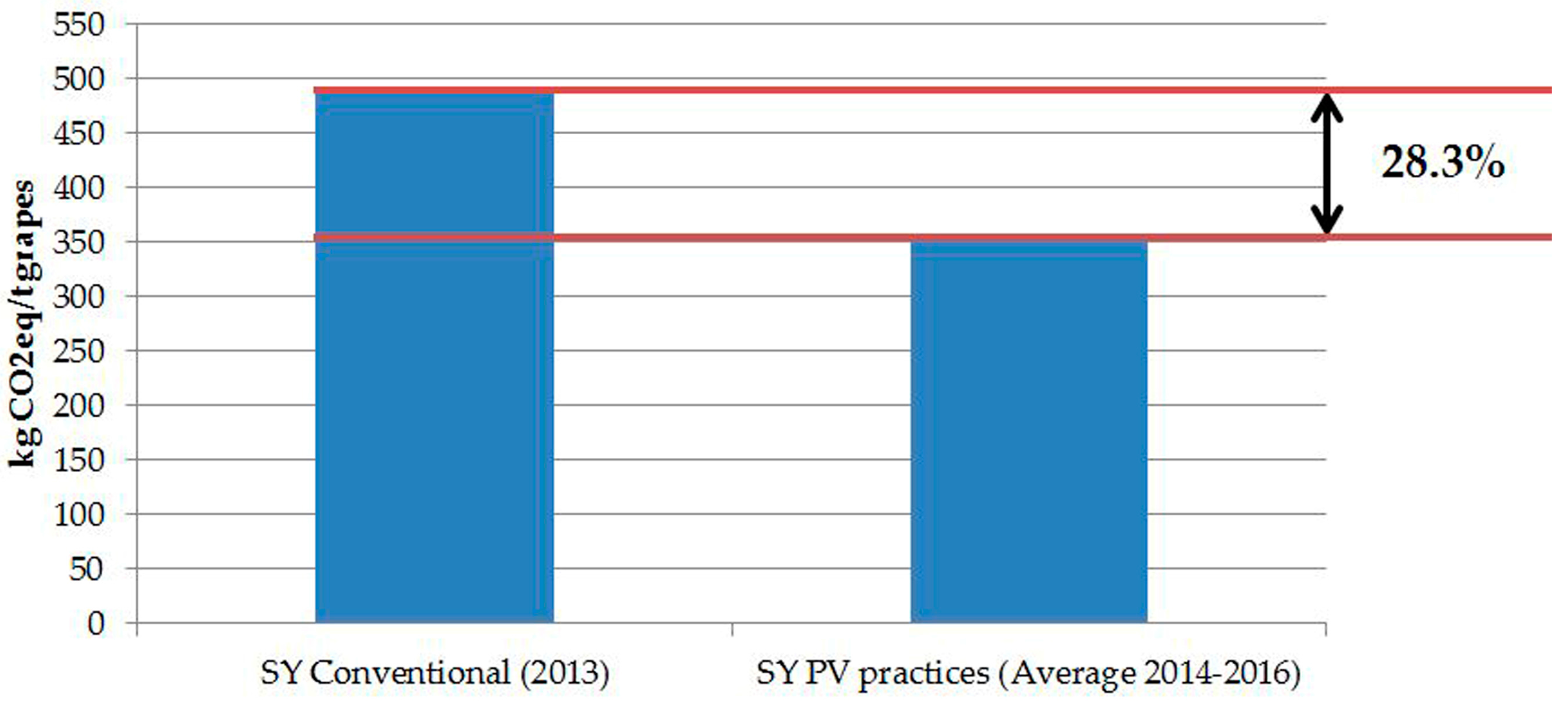
The SY vineyard showed a different profile than the SB vineyard regarding PCF. In the 2013 vintage, the total GHG emissions were much lower in surface basis in comparison to the SB vineyard (3443.3 vs. 5744.1 kg CO2/ha) due to less-intensive practices, but the yield was also significantly less (7 vs. 12.7 t/ha), leading to a higher final PCF for SY that reached 491.1 kg CO2/t grapes in comparison to SB (452.6 kg CO2/t grapes). After PV practices in the three consecutive vintages, the PCF was 351.9 kg CO2/t grapes, which reduced emissions by 139.16 kg CO2eq/t grapes (28.3%) as shown in Figure 9.
The paired sample t-tests showed that PCF values were lower for all consecutive years in comparison to 2013, with p < 0.05 statistical significance (95% confidence interval of the difference). As for the Q-tests, it was shown that the frequency of PCF values in the three consecutive seasons that were lower than the respective values in 2013 (shown as 0) was not significantly different from the conventional method over the three PV seasons (Table 7).
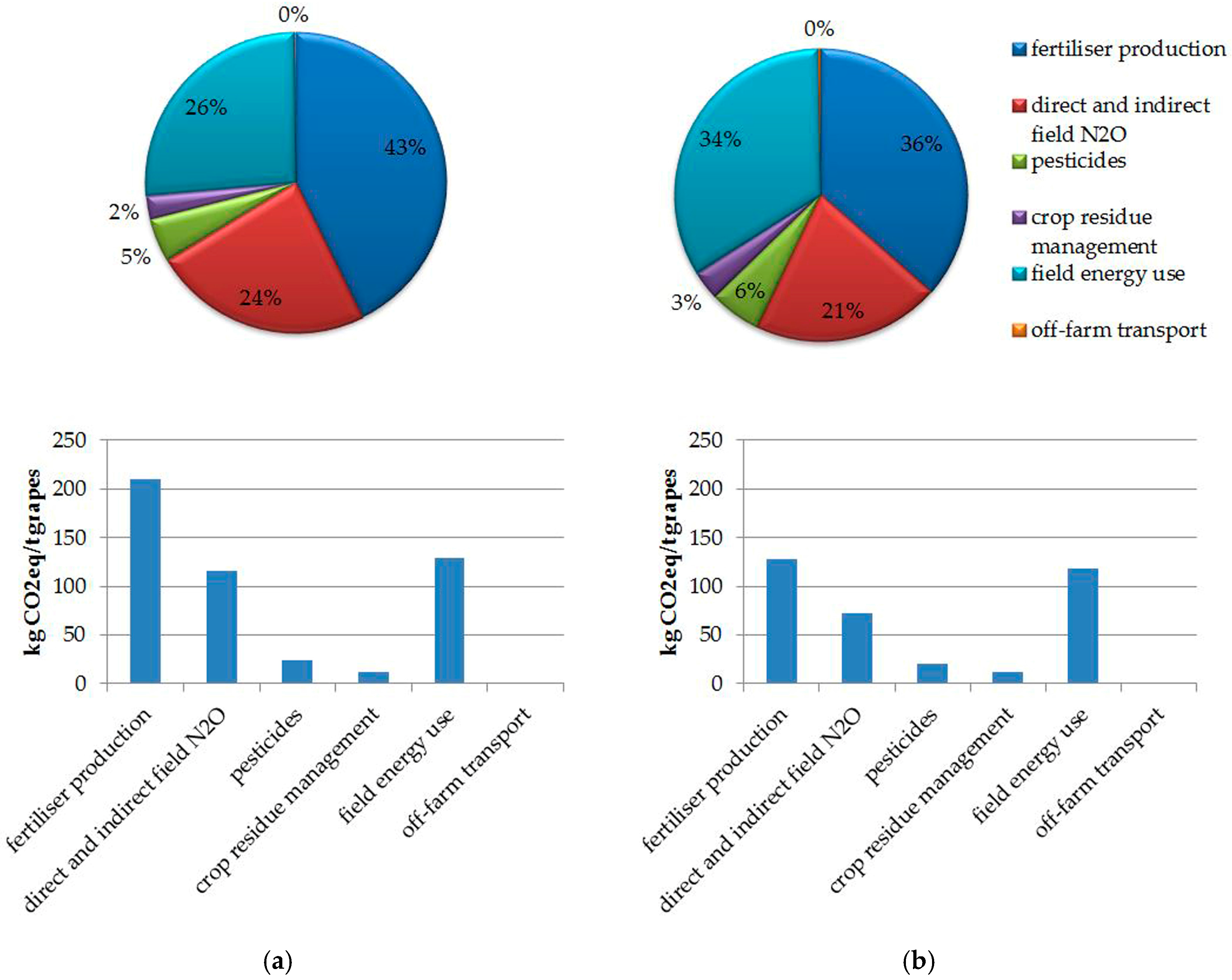
The distribution of emissions among the agricultural practices in the SY vineyard followed a different trend than the SB vineyard (Figure 10). The reason was that SY received less tillage, pesticide application, and irrigation than SB, which decreased the impact of energy use (electricity and fuel) within the vineyard. Therefore, the most significant activity regarding GHG emissions was fertilizer production and distribution in both conventional and PV practices, reaching 209.5 kg CO2eq/t grapes (42.7%) and 128.3 kg CO2eq/t grapes (36.5%), respectively. The decrease of GHGs of this activity between conventional and PV practices was 38.7%.
Nitrogen fertilizers and manure application were also responsible for direct and indirect N2O emissions of 116.2 (23.7%) and 72.8 kg CO2eq/t grapes (20.7%) of the GHG emissions in conventional and PV practices. Hence, fertilization as a total (production and application) counted for 325.7 (66.3%) and 201.2 kg CO2eq/t grapes (57.2%) of the emissions in the SY vineyard following the two practices under study. The PV application reduced the impact of fertilizer use on the total GHG emissions by 25.4%, showing that in less-intensive vineyards precise fertilization can make an even greater difference in potential global warming mitigation.
Even if field energy is less important in terms of GHG emissions, it still plays a significant role in both conventional and PV practices, counting for 128.7 and 118.4 kg CO2eq/t grapes, respectively (26.2% and 33.6% of the total GHG emissions). It was observed that the increase in irrigation (8.3%) after PV techniques did not have a negative impact on the PCF, as the increase of yield (16%) compensated electricity augmentation for water pumping. As in SB, fuel use stayed almost unaffected, counting for 25.9 kg CO2eq/t grapes (5.3% of total GHGs) in 2013 vintage and 22.4 kg CO2eq/t grapes (6.5% of total GHGs).
Crop residues management emissions (soil incorporation of trimmed canes) decreased from 12.2 to 11.3 kg CO2eq/t grapes when moving from conventional to PV practices, counting for 2.5% and 3.2% of the total GHG emissions for each vintage. PV practices increased canes by 6.6% due to better use of nutrients and water, but yield increase (16%) reversed the situation. Pesticide application emissions were reduced from 23.4 to 20.2 kg CO2eq/t grapes (4.8% and 5.7% for each practice, respectively), due to yield increase during the PV practices. Similarly to SB, off-farm transportation covered 0.2–0.3% of the total GHG emissions of the SY vineyard, as it is only attributed to 5-km transport of grapes within the premises of the winery.

4. Discussion

This study compares the conventional practices that were carried out in one vintage period (2013) with PV practices that followed in the next three consecutive vintages (2014–2016). Differences in the average rainfall and temperatures between the vintages under study caused discrepancies in critical stages that were responsible for variations in the final yield, impacting the LCA calculations among the years. The fact that multiple growing seasons are examined—where the year effect cannot impact as a major factor in the LCA analysis—makes this work provide stable results based on average values of multi-seasonal variable rate application of nutrients and irrigation water. The importance of this study was to show the influence on the reduction of GHG emissions both from different vineyard cultivars in the same region that receive different numbers of operations, and also the effect of different management zones, which is the cornerstone of precision agriculture.
From the two vineyard cultivars under study applying variable rate fertilizers and irrigation water, it is evident that the main GHG reduction came from fertilizers and energy use. SB contribution to GHG emissions was significantly higher than SY on a surface basis (40%) using conventional practices (5744 kg CO2eq/ha vs. 3443 kg CO2eq/ha), because a larger number of practices was carried out in comparison to SY. This is an indication that presents the effect of a higher number of practices per vineyard cultivar in the reduction of GHGs. The decrease of the GHG emissions from both vineyards after PV practices on a surface basis (where the impact of yield is not included) was higher in SB (23%) than in SY (17%), reflecting the higher impact of less agricultural inputs in more intensive cultivation systems. Literature does not provide information on the global warming potential of precision viticulture practices. However, similar statements have been given by studies focusing on organic viticulture that is again a comparison between existing agricultural practices and a new production system, and could enforce the results of this paper. Rouault et al. (2016) pointed out that some emission models need to be improved to better assess the environmental impacts of viticulture and that soil quality should also be integrated in the analysis, as its absence may be a disadvantage for organic viticulture [34]. This comes in accordance with Kavargiris et al. (2009), who found that GHGs were significantly higher in all cultivation practices except pruning in conventional viticulture compared to organic viticulture [53]. Moreover, according to their study, pruning presented significantly higher GHG emissions in the organic viticulture. Rugani (2013) concluded that a wide range of issues related to wine PCF remain unexplored [25]. In addition, Venkat (2012) indicated that vineyard machinery use accounted for more than 60% of the total global warming potential [37]. The latter comes in accordance with Longbottom and Petrie (2015), who stated that fuel and electricity use are responsible for almost 98% of the total GHG emissions in viticulture [54]. The average net global warming potential was 158 g CO2eq/kg for conventional grapes and was reduced to 113 g CO2eq/kg under organic management [37]. Moreover, viticulture has the largest environmental impact in the whole wine value chain according to Neto et al. (2013) [55].
This experimental work showed that applying variable rate application of fertilizers and water in a vineyard based on the actual requirements of different in-field zones can reduce significantly GHG emissions derived from viticulture. Such practices can show a potential for environmental benefits in combination with the positive results on quantitative and qualitative parameters. Therefore, research in PV should not only look at the effect in yield and optimization of resources, but also in the reduction of emissions, which is a vital part of the field variability. As stated above, studies focusing on the environmental impact of precision agriculture are very scarce, and future work should also look at this aspect apart from the agronomic and economic effects [56].

5. Conclusions

Precision viticulture has evolved significantly in recent years, and it has indications of increasing the production quality and quantity, with a positive impact on vineyard economics as well. However, the environmental impact, and more specifically the potential effect on global warming from the application of such practices, was not analysed thoroughly in literature.
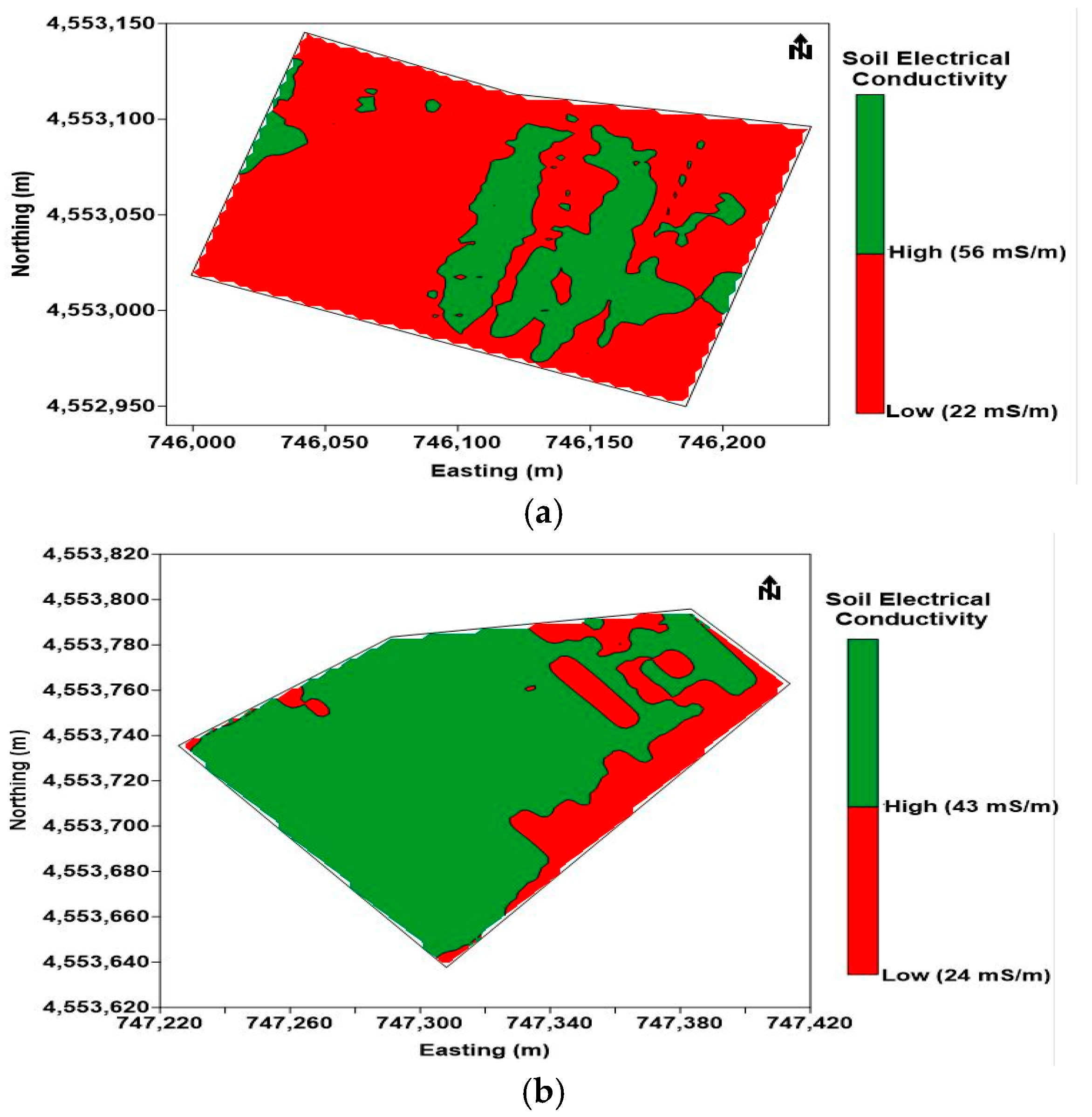
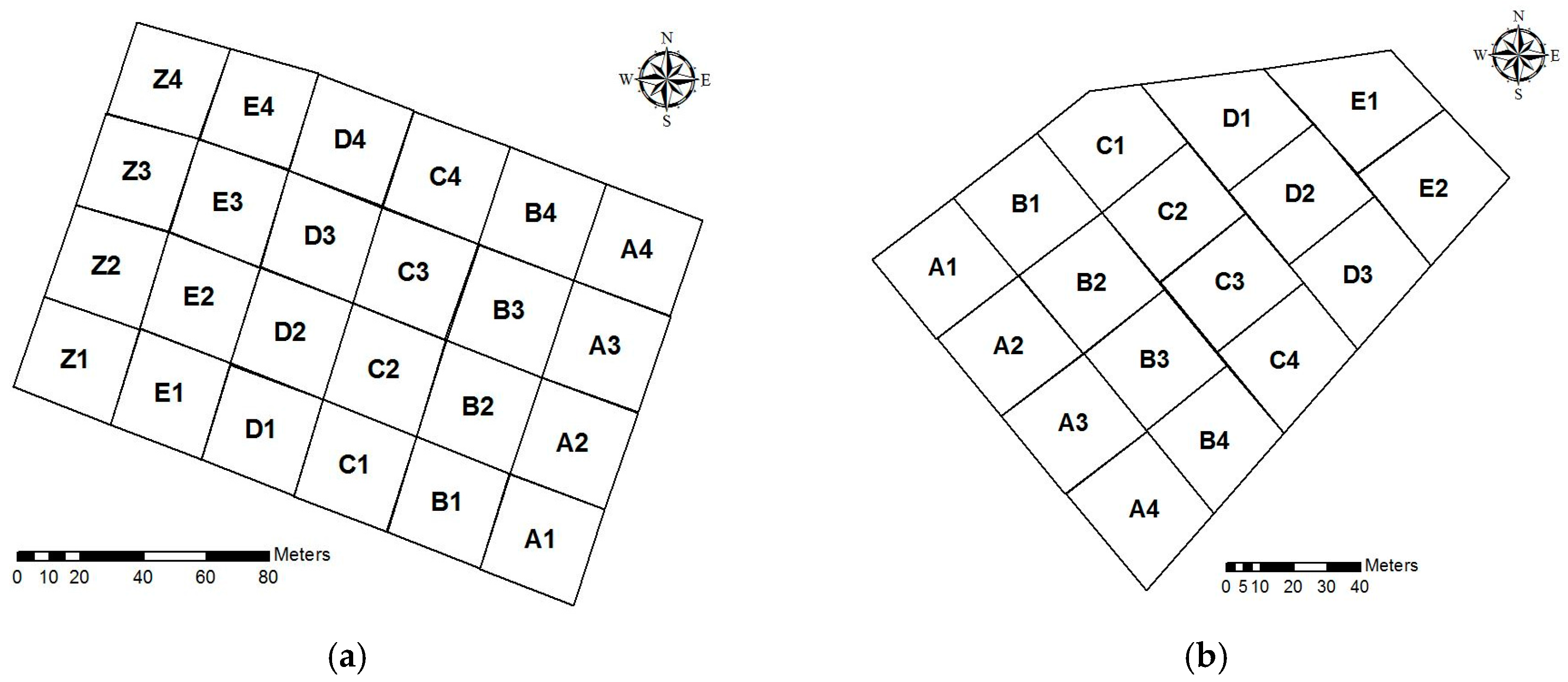
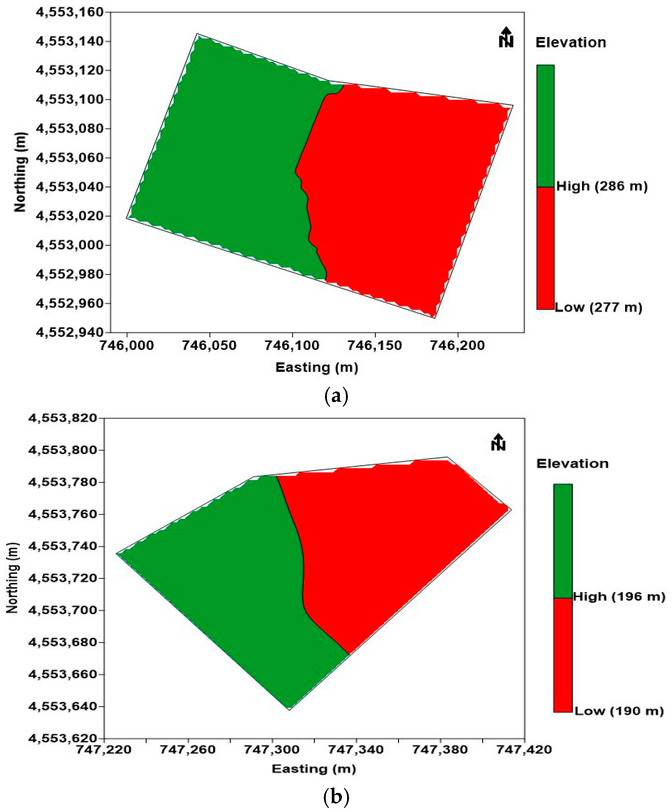
In this work, a life cycle assessment of the production system of two vineyards in Northern Greece planted with different cultivars of wine vines (Sauvignon Blanc and Syrah) was executed for two production systems during four growing seasons, where in 2013 conventional practices were applied and in the consecutive years (2014, 2015, and 2016) it was selected to regulate irrigation and fertilizer application according to precision viticulture techniques. Two management zones were delineated for each vineyard, and different water and fertilizer quantities were applied to each zone according to vigour analysis of the vines canopy. After assembling a detailed inventory of inputs and outputs of the vineyards for both conventional and PV practices, a deterministic analysis of the emitted GHG emissions from each agricultural practice was carried out, and suggested that PV application can significantly reduce GHG emission derived by wine grape production.

Acknowledgments

This study was funded by the General Secretariat for Research and Technology Greece (G.S.R.T.) under the project titled “Green Vineyard”.

Author Contributions

All authors conceived the idea of the paper and designed the experiments; Evangelos Anastasiou, Stefanos Koundouras, Athanasios Balafoutis and Spyros Fountas performed the field experiments in the two vineyards; Athanasios Balafoutis and Evangelos Anastasiou analyzed the data; Konstantinos Arvanitis and Spyros Fountas contributed with their experience in the analysis and presentation of data; Athanasios Balafoutis performed the LCA.

Conflicts of Interest

The authors declare no conflict of interest. The founding sponsors had no role in the design of the study; in the collection, analyses, or interpretation of data; in the writing of the manuscript, and in the decision to publish the results.

References

  1. Tilman, D.; Fargione, J.; Wolff, B.; D’Antonio, C.; Dobson, A.; Howarth, R.; Schindler, D.; Schlesinger, W.H.; Simberloff, D.; Swackhamer, D. Forecasting agriculturally driven global environmental change. Science 2001, 292, 281–284. [Google Scholar] [CrossRef] [PubMed]
  2. Lal, R. Soil Carbon Sequestration Impacts on Global Climate Change and Food Security. Science 2004, 304, 1623–1627. [Google Scholar] [CrossRef] [PubMed]
  3. Montgomery, D.R. Soil erosion and agricultural sustainability. Proc. Natl. Acad. Sci. USA 2007, 104, 13268–13272. [Google Scholar] [CrossRef] [PubMed]
  4. Lal, R. Enhancing Eco-Efficiency in Agro-Ecosystems through Soil Carbon Sequestration. Crop Sci. 2010, 50, 120–131. [Google Scholar] [CrossRef]
  5. Quinton, J.N.; Govers, G.; Van Oost, K.; Bardgett, R.D. The impact of agricultural soil erosion on biogeochemical cycling. Nat. Geosci. 2010, 3, 311–314. [Google Scholar] [CrossRef] [Green Version]
  6. Robertson, G.P.; Vitousek, P.M. Nitrogen in agriculture: Balancing the cost of an essential resource. Ann. Rev. Environ. Resour. 2009, 34, 97–125. [Google Scholar] [CrossRef]
  7. Vitousek, P.M.; Naylor, R.; Crews, T.; David, M.B.; Drinkwater, L.E.; Holland, E.; Johnes, P.J.; Katzenberger, J.; Martinelli, L.A.; Matson, P.A.; et al. Nutrient Imbalances in Agricultural Development. Science 2009, 324, 1519–1520. [Google Scholar] [CrossRef] [PubMed]
  8. Morison, J.I.L.; Baker, N.R.; Mullineaux, P.M.; Davies, W.J. Improving water use in crop production. Philos. Trans. R. Soc. B Biol. Sci. 2008, 363, 639–658. [Google Scholar] [CrossRef] [PubMed]
  9. Stoate, C.; Báldi, A.; Beja, P.; Boatman, N.D.; Herzon, I.; Van Doorn, A.; De Snoo, G.R.; Rakosy, L.; Ramwell, C. Ecological impacts of early 21st century agricultural change in Europe—A review. J. Environ. Manag. 2009, 91, 22–46. [Google Scholar] [CrossRef] [PubMed]
  10. Hernández, A.F.; Parrón, T.; Tsatsakis, A.M.; Requena, M.; Alarcón, R.; López-Guarnido, O. Toxic effects of pesticide mixtures at a molecular level: Their relevance to human health. Toxicology 2013, 307, 136–145. [Google Scholar] [CrossRef] [PubMed]
  11. Montzka, S.A.; Dlugokencky, E.J.; Butler, J.H. Non-CO2 greenhouse gases and climate change. Nature 2011, 476, 43–50. [Google Scholar] [CrossRef] [PubMed]
  12. MacLeod, M.; Eory, V.; Gruere, G.; Lankoski, J. Cost-Effectiveness of Greenhouse Gas Mitigation Measures for Agriculture; OECD Publishing: Paris, France, 2015; Volume 89. [Google Scholar]
  13. Colomb, V.; Bernoux, M.; Bockel, L.; Chotte, J.L.; Martin, S.; Martin-Phipps, C.; Mousset, J.; Tinlot, M.; Touchemoulin, O. Review of GHG Calculators in Agriculture and Forestry Sectors. Available online: http://www.fao.org/fileadmin/templates/ex_act/pdf/ADEME/Review_existingGHGtool_VF_UK4.pdf (accessed on 12 June 2017).
  14. Notarnicola, B.; Tassielli, G.; Nicoletti, G. Life cycle assessment (LCA) of wine production. Environ. Friendly Food Process. 2003, 306, 326. [Google Scholar]
  15. Jiménez, E.; Martínez, E.; Blanco, J.; Pérez, M.; Graciano, C. Methodological approach towards sustainability by integration of environmental impact in production system models through life cycle analysis: Application to the Rioja wine sector. Simulation 2014, 90, 143–161. [Google Scholar] [CrossRef]
  16. Guinée, J.B. Handbook on life cycle assessment operational guide to the ISO standards. Int. J. Life Cycle Assess. 2002, 7, 311–313. [Google Scholar] [CrossRef]
  17. Milà i Canals, L.; Burnip, G.; Suckling, D.; Cowell, S. Sources of Site-Dependency and Importance of Energy Consumption in Agricultural LCA: Apple Production in New Zealand. DIAS Repeport. Proceedings of the International Conference, Munich, Germany, 26–30 July 2004; pp. 236–240. [Google Scholar]
  18. Nemecek, T.; Heil, A.; Huguenin, O.; Meier, S.; Erzinger, S.; Blaser, S.; Dux, D.; Zimmermann, A. Life Cycle Inventories of Agricultural Production Systems; Final Report Ecoinvent v2.0 No. 15a; Agroscope Reckenholz-Taenikon Research Station ART, Swiss Centre for Life Cycle Inventories: Zurich/Dübendorf, Switzerland, 2007. [Google Scholar]
  19. Christ, K.L.; Burritt, R.L. Critical environmental concerns in wine production: An integrative review. J. Clean. Prod. 2013, 53, 232–242. [Google Scholar] [CrossRef]
  20. Bosco, S.; Di Bene, C.; Galli, M.; Remorini, D.; Massai, R.; Bonari, E. Greenhouse gas emissions in the agricultural phase of wine production in the Maremma rural district in Tuscany, Italy. Ital. J. Agron. 2011, 6, 15. [Google Scholar] [CrossRef] [Green Version]
  21. Point, E.; Tyedmers, P.; Naugler, C. Life cycle environmental impacts of wine production and consumption in Nova Scotia, Canada. J. Clean. Prod. 2012, 27, 11–20. [Google Scholar] [CrossRef]
  22. Vázquez-Rowe, I.; Rugani, B.; Benetto, E. Tapping carbon footprint variations in the European wine sector. J. Clean. Prod. 2013, 43, 146–155. [Google Scholar] [CrossRef]
  23. Litskas, V.D.; Irakleous, T.; Tzortzakis, N.; Stavrinides, M.C. Determining the carbon footprint of indigenous and introduced grape varieties through Life Cycle Assessment using the island of Cyprus as a case study. J. Clean. Prod. 2017, 156, 418–425. [Google Scholar] [CrossRef]
  24. Pattara, C.; Russo, C.; Antrodicchia, V.; Cichelli, A. Carbon footprint as an instrument for enhancing food quality: Overview of the wine, olive oil and cereals sectors. J. Sci. Food Agric. 2016, 97, 396–410. [Google Scholar] [CrossRef] [PubMed]
  25. Rugani, B.; Vázquez-Rowe, I.; Benedetto, G.; Benetto, E. A comprehensive review of carbon footprint analysis as an extended environmental indicator in the wine sector. J. Clean. Prod. 2013, 54, 61–77. [Google Scholar] [CrossRef]
  26. Bellon-Maurel, V.; Peters, G.M.; Clermidy, S.; Frizarin, G.; Sinfort, C.; Ojeda, H.; Roux, P.; Short, M.D. Streamlining life cycle inventory data generation in agriculture using traceability data and information and communication technologies—Part II: Application to viticulture. J. Clean. Prod. 2015, 87, 119–129. [Google Scholar] [CrossRef]
  27. Adewale, C.; Higgins, S.; Granatstein, D.; Stöckle, C.O.; Carlson, B.R.; Zaher, U.E.; Carpenter-Boggs, L. Identifying hotspots in the carbon footprint of a small scale organic vegetable farm. Agric. Syst. 2016, 149, 112–121. [Google Scholar] [CrossRef]
  28. Marras, S.; Masia, S.; Duce, P.; Spano, D.; Sirca, C. Carbon footprint assessment on a mature vineyard. Agric. For. Meteorol. 2015, 214, 350–356. [Google Scholar] [CrossRef]
  29. Eldon, J.; Gershenson, A. Effects of cultivation and alternative vineyard management practices on soil carbon storage in diverse Mediterranean landscapes: A review of the literature. Agroecol. Sustain. Food Syst. 2015, 39, 516–550. [Google Scholar] [CrossRef]
  30. Brunori, E.; Farina, R.; Biasi, R. Sustainable viticulture: The carbon-sink function of the vineyard agro-ecosystem. Agric. Ecosyst. Environ. 2016, 223, 10–21. [Google Scholar] [CrossRef]
  31. Litskas, V.D.; Karaolis, C.S.; Menexes, G.C.; Mamolos, A.P.; Koutsos, T.M.; Kalburtji, K.L. Variation of energy flow and greenhouse gas emissions in vineyards located in Natura 2000 sites. Ecol. Indic. 2013, 27, 1–7. [Google Scholar] [CrossRef]
  32. Steenwerth, K.L.; Strong, E.B.; Greenhut, R.F.; Williams, L.; Kendall, A. Life cycle greenhouse gas, energy, and water assessment of wine grape production in California. Int. J. Life Cycle Assess. 2015, 20, 1243–1253. [Google Scholar] [CrossRef]
  33. Gabzdylova, B.; Raffensperger, J.F.; Castka, P. Sustainability in the New Zealand wine industry: Drivers, stakeholders and practices. J. Clean. Prod. 2009, 17, 992–998. [Google Scholar] [CrossRef]
  34. Rouault, A.; Beauchet, S.; Renaud-Gentie, C.; Jourjon, F. Life Cycle Assessment of viticultural technical management routes (TMRs): Comparison between an organic and an integrated management route. OENO One 2016, 50. [Google Scholar] [CrossRef]
  35. Villanueva-Rey, P.; Vázquez-Rowe, I.; Moreira, M.T.; Feijoo, G. Comparative life cycle assessment in the wine sector: Biodynamic vs. conventional viticulture activities in NW Spain. J. Clean. Prod. 2014, 65, 330–341. [Google Scholar] [CrossRef]
  36. Vázquez-Rowe, I.; Villanueva-Rey, P.; Iribarren, D.; Moreira, M.T.; Feijoo, G. Joint life cycle assessment and data envelopment analysis of grape production for vinification in the Rías Baixas appellation (NW Spain). J. Clean. Prod. 2012, 27, 92–102. [Google Scholar] [CrossRef]
  37. Venkat, K. Comparison of twelve organic and conventional farming systems: A life cycle greenhouse gas emissions perspective. J. Sustain. Agric. 2012, 36, 620–649. [Google Scholar] [CrossRef]
  38. Aguilera, E.; Guzmán, G.; Alonso, A. Greenhouse gas emissions from conventional and organic cropping systems in Spain. II. Fruit tree orchards. Agron. Sustain. Dev. 2015, 35, 725–737. [Google Scholar] [CrossRef]
  39. Bramley, R.G.V.; Pearse, B.; Chamberlain, P. Being profitable precisely—A case study of precision viticulture from Margaret River. Aust. N. Z. Grape Grow. Winemak. 2003, 473, 84–87. [Google Scholar]
  40. Kitchen, N.R.; Sudduth, K.A.; Myers, D.B.; Drummond, S.T.; Hong, S.Y. Delineating productivity zones on claypan soil fields using apparent soil electrical conductivity. Comput. Electron. Agric. 2005, 46, 285–308. [Google Scholar] [CrossRef]
  41. Tagarakis, A.; Chatzinikos, A.; Fountas, S.; Gemtos, T. Delineation of Management Zones in Precision Viticulture. In Proceedings of the 3rd International Conference on HAICTA (Information Systems in Sustainable Agriculture, Agroenvironment and Food Technology), Volos, Greece, 20–23 September 2006. [Google Scholar]
  42. Groeneveld, D.P.; Baugh, W.M.; Sanderson, J.S.; Cooper, D.J. Annual groundwater evapotranspiration mapped from single satellite scenes. J. Hydrol. 2007, 344, 146–156. [Google Scholar] [CrossRef]
  43. Dry, P.R.; Loveys, B.R.; McCarthy, M.G.; Stoll, M. Strategic irrigation management in Australian vineyards. J. Int. Sci. Vigne Vin 2001, 35, 129–139. [Google Scholar] [CrossRef]
  44. Christensen, P.L.; Peacock, W.L. Mineral nutrition and fertilization. In Raisin Production Manual; Christensen, L.P., Ed.; Communication Services-Publications; Division of Agricultural and Natural Resources, University of California: Oakland, CA, USA, 2000; pp. 102–114. [Google Scholar]
  45. Ganeshamurthy, A.N.; Satisha, G.C.; Patil, P. Potassium nutrition on yield and quality of fruit crops with special emphasis on banana and grapes. Karnataka J. Agric. Sci. 2011, 1, 29–38. [Google Scholar]
  46. Whittaker, C.; McManus, M.C.; Smith, P. A comparison of carbon accounting tools for arable crops in the United Kingdom. Environ. Model. Softw. 2013, 46, 228–239. [Google Scholar] [CrossRef] [Green Version]
  47. IPCC Revised Good Practice Guidelines for Greenhouse Gas Inventories. Available online: http://www.ipcc-nggip.iges.or.jp/public/2006gl/vol4.html (accessed on 24 May 2017).
  48. Hillier, J.; Walter, C.; Malin, D.; Garcia-Suarez, T.; Mila-i-Canals, L.; Smith, P. A farm-focused calculator for emissions from crop and livestock production. Environ. Model. Softw. 2011, 26, 1070–1078. [Google Scholar] [CrossRef]
  49. European Life Cycle Database. Available online: http://eplca.jrc.ec.europa.eu/ELCD3/datasetDownload.xhtml (accessed on 1 August 2017).
  50. Bouwman, A.F.; Boumans, L.J.M.; Batjes, N.H. Modeling Global Annual N2O and NO Emissions from Fertilized Fields. Glob. Biogeochem. Cycles 2002, 16, 1080–1107. [Google Scholar] [CrossRef]
  51. Audsley, E. Harmonisation of Environmental Life Cycle Assessment for Agriculture; European Commission, DG VI Agriculture: Brussels, Belgium, 1997; p. 139. [Google Scholar]
  52. Greenhouse Gas Protocol. Available online: www.ghgprotocol.org (accessed on 2 August 2017).
  53. Kavargiris, S.E.; Mamolos, A.P.; Tsatsarelis, C.A.; Nikolaidou, A.E.; Kalbourtji, K.L. Energy resources' utilization in organic and conventional vineyards: Energy flow, greenhouse gas emissions and biofuel production. Biomass Bioenergy 2009, 33, 1239–1250. [Google Scholar] [CrossRef]
  54. Longbottom, M.L.; Petrie, P.R. Role of vineyard practices in generating and mitigating greenhouse gas emissions. Aust. J. Grape Wine Res. 2015, 21, 522–536. [Google Scholar] [CrossRef]
  55. Neto, B.; Dias, A.C.; Maachado, M. Life cycle assessment of the supply chain of a Portuguese wine: From viticulture to distribution. Int. J. Life Cycle Assess. 2013, 18, 590–602. [Google Scholar] [CrossRef]
  56. Balafoutis, A.; Beck, B.; Fountas, S.; Vangeyte, J.; Van de Wal, T.; Soto-Embodas, I.; Gomes-Barbero, M.; Barnes, A.P.; Eory, V. Precision Agriculture Technologies Positively Contributing to GHG Emissions Mitigation, Farm Productivity and Economics. Sustainability 2017, 9, 1339. [Google Scholar] [CrossRef]
Figure 1. Satellite image and boundaries of (a) Sauvignon Blanc vineyard; (b) Syrah vineyard.
Sustainability 09 01997 g001
Figure 2. Grid cells of (a) Sauvignon Blanc vineyard; (b) Syrah vineyard.
Sustainability 09 01997 g002
Figure 3. Soil Electrical Conductivity (ECa) of (a) Sauvignon Blanc vineyard; (b) Syrah vineyard.
Sustainability 09 01997 g003
Figure 4. Elevation of (a) Sauvignon Blanc vineyard; (b) Syrah vineyard.
Sustainability 09 01997 g004
Figure 5. Management zones of (a) Sauvignon Blanc vineyard; (b) Syrah vineyard.
Sustainability 09 01997 g005
Figure 6. Vineyard input/output flow.
Sustainability 09 01997 g006
Figure 7. Total GHG emission of Sauvignon Blanc (SB) for the conventional and precision viticulture practices.
Sustainability 09 01997 g007
Figure 8. Emission distribution among practices in Sauvignon Blanc (a) conventional; (b) precision viticulture.
Sustainability 09 01997 g008
Figure 9. Total GHG emission of Syrah (SY) for the conventional and precision viticulture practices.
Sustainability 09 01997 g009
Figure 10. Emission distribution among practices in Syrah (a) conventional; (b) precision viticulture.
Sustainability 09 01997 g010
Table 1. Conventional practices and respective inputs/outputs for Sauvignon Blanc and Syrah vineyards.
OperationsInput/OutputUnitSauvignon BlancSyrah
ActionsQuantity/haActionsQuantity/ha
Row tillage with intra-row mowingFuelkg418.4313.8
TillageFuelkg13.913.9
TrimmingFuelkg36.124.1
Fertilization (fertigation)NH4NO3kg25972597
K2SO4kg22502250
Manure applicationSheep manuret130130
Fuelkg16.716.7
SprayingCopperg311322562
Wet sulphurg12001200
Slashcm3190.5190.5
Delang11811181
Teldorg13621362
Polyramg15701570
Flintg157157
Teldorg1570--
Fuelkg1160.2839.3
DustingSulphurkg125--
Fuelkg10.3
IrrigationWaterm31030004800
ElectricitykWh37501000
PruningWood weightt13.411.2
YieldGrapest112.717.01
Table 2. Normalized Difference Vegetation Index (NDVI) at veraison stage for three consecutive years after precision viticulture (PV) practices.
Sauvignon Blanc
ZoneYearMinMaxMeanStD
120160.6750.7760.7340.034
20150.7020.7400.7240.011
20140.6880.7300.7120.012
220160.7060.8350.7670.039
20150.7200.8200.7710.031
20140.7220.7650.7410.015
Syrah
120160.6200.7040.6640.035
20150.6200.6860.6500.023
20140.6150.6860.6470.023
220160.7360.7850.7660.018
20150.7220.8190.7690.027
20140.7300.7790.7570.018
Table 3. Precision viticulture practices and respective inputs/outputs for Sauvignon Blanc and Syrah vineyards in each zone per ha.
Parameter Input/Output per haUnitSauvignon BlancSyrah
Zone 1Zone 2Zone 1Zone 2
Fertilization (fertigation)2014NH4NO3kg388298.5567.1298.6
K2SO4250312.5312.5375
2015NH4NO3358.2268.7567.1283.6
K2SO465754545
2016NH4NO3343.3283.6537.3283.6
K2SO456703845
AverageNH4NO3363.2283.6557.2288.6
K2SO4123.7152.5131.8155
Irrigation2014Waterm3300020001200600
ElectricitykWh375025001500750
2015Waterm3260018001000500
ElectricitykWh325022501250625
2016Waterm3320024001400800
ElectricitykWh4000300017501000
AverageWaterm32933.32066.71200633.3
ElectricitykWh3666.72583.31500791.7
Pruning2014Wood weightt4.064.771.051.53
20154.175.11.221.62
20163.844.280.861.29
Average4.024.721.041.48
Yield2014Grapest12.2214.388.179.04
201512.4214.528.048.58
201610.8113.547.037.57
Average11.8214.157.758.4
Table 4. Meteorological data for the growing seasons of the experiment.
Growing SeasonMean Temperature (°C)Total Precipitation (mm)
201317.5725
201418.3990
201518.31088
201618.6840
Table 5. Agricultural practices in viticulture and the respective greenhouse gas (GHG) emissions.
Agricultural PracticeType of GHG Measured
Fertilizers production and distributionAll types of GHG emissions from these processes 1
Nitrogen fertilisers and manure applicationN2O, NO, and NH3 soil emissions from N application and transformation processes of N in soils 2
Pesticide production and distributionAll types of GHG emissions from these processes 3
Tillage, Spraying, Dusting, Fertilizer and Manure application, Pruning, Transportation (on- and off-farm)CO2 from fuel use in tractor 4
IrrigationCO2 from electricity use for pumping water 5
1 Emissions are inventoried in the European Life Cycle Database (ELCD) core database for the current technology of fertilizer production [49]. 2 N-related soil emissions were calculated using the model of Bouwman et al. (2002) [50]. 3 The combined average emissions from different pesticide types comes from Audsley (1997) [51]. 4 Diesel fuel emissions were calculated according to www.ghgprotocol.org [52]. 5 Electricity energy mix for Greece was used coming from IEA CO2 Highlights for countries and regions.
Table 6. Agricultural practices in viticulture and the respective greenhouse gas emissions.
Frequencies
Value
01
2014222
2015231
2016204
Test Statistics
N24
χ24.667 a
p0.097
a 0 is treated as a success.
Table 7. Agricultural practices in viticulture and the respective greenhouse gas emissions.
Frequencies
Value
01
2014161
2015152
2016161
Test Statistics
N17
χ22.000 a
p0.368
a 0 is treated as a success.

