A Long-Term Assessment of the Black Sea Wave Climate


Department of Mechanical Engineering, Faculty of Engineering, “Dunărea de Jos” University of Galati, 47 Domneasca Street, 800008 Galati, Romania
*
Author to whom correspondence should be addressed.
Sustainability 2017, 9(10), 1875; https://doi.org/10.3390/su9101875
Submission received: 12 September 2017
/
Revised: 4 October 2017
/
Accepted: 16 October 2017
/
Published: 18 October 2017
(This article belongs to the Section Environmental Sustainability and Applications)
Abstract
:In the present work the Black Sea wave climate is assessed using a total of 38 years of data (1979–2016). As a first step, the long-term variations of the main wave parameters were evaluated using data provided by the European Center for Medium-Range Weather Forecasts (ECMWF). Based on these values, the nearshore and offshore conditions from the Black Sea were evaluated. Moreover, the Sea of Azov was also targeted in this study, since in some cases the conditions are comparable with those of the Black Sea. Going up to the present day, the regional wave climate was assessed through satellite measurements provided by the AVISO project, at the same time indicating the differences between these data and the ECMWF reanalysis dataset. In general, the conditions reported in the northwestern sector of the Black Sea seem to be more energetic, indicating more frequently the presence of rough conditions. Finally, it can be concluded that the results presented in the present study cover a broad range of applications in climatological studies and other types of research related to coastal protection.
1. Introduction
Global warming and the sea-level rise are clear indicators of climatological changes. There are increasing voices that consider that these changes are related to human activities, as it has been estimated that since the Industrial Revolution CO2 emissions have increased by almost 40%, which subsequently raised the global average temperature by almost 0.8 °C [1]. If we discuss the climate system, we need to mention the interconnected atmosphere and ocean environments, which constantly exchange water and energy [2,3]. Marine areas seem to be more sensitive to these variations, revealing the destructive forces of some extreme events, as in the case of Hurricane Katrina [4]. For low-lying areas, coastal flooding represents a real threat, being caused by the joint action of wind, waves, and tidal forces, which considerably increase in magnitude during storm events [5]. Coastal erosion represents another key issue for beach sectors, which can be attenuated through conventional or innovative protection schemes [6,7,8].
As expected, the marine environment is defined by large water areas that are difficult to monitor with moored buoy instruments, which are the property of national or international research institutes. In discussing the wave characteristics, a common practice is to use past wind data in order to force a numerical wave model or an artificial neural network to generate hindcast estimations [9]. Various reanalysis projects were developed overtime, of which we might mention Reanalysis I, maintained by the National Centers for Environmental Prediction/National Center for Atmospheric Research, or the JRA-55 project developed by the Japanese Meteorological Society. Another major project is ERA40 (covering 45 years of data: September 1979–August 2002), maintained by the ECMWF, which was replaced by the ERA-Interim project (started in 1989) that is used in the current work to assess wave conditions from the Black Sea [10,11,12].
The Black Sea is considered a dynamic environment that is subjected to seasonal variations induced by regional atmospheric features. This basin is considered to be a semi-enclosed sea, connected to the Mediterranean Sea through the Straits of Dardanelles and Bosporus, located in the northeast sector of the sea. In terms of the drainage basin, the hydrographic network is the largest one from Europe. Thus, some major rivers such as the Danube or Don [13] can be mentioned. The general weather pattern is influenced by North Atlantic cyclones and anticyclones that arrive in this area of the Mediterranean Sea, while on a local scale the presence of the Caucasus and Crimean mountains generates mesoscale disturbances. It was estimated that in the case of the Caucasian cyclones, the surface wind has a northern or northeastern orientation over the land, while a northwestern pattern was reported over the sea in the vicinity of the Caucasian coast. The lifetime of the Caucasian vortices was estimated to be around 10 h, covering a horizontal and vertical scale of 100 km and 1.5–2 km, respectively, during which the wind speed may report values in the range of 5–10 m/s [14,15]. On a local scale, the breeze circulation represents another important event that modifies the bottom layers of the atmosphere, being generated by the diurnal variations of the sea–land temperature. As expected, the Black Sea circulation is influenced by the presence of the mountains and by the coastline morphology, with it being estimated that the nighttime breeze is weaker than the diurnal one [16]. Previous studies suggest that the northern part of the sea reports more significant wind resources, especially in the vicinity of Romania and Ukraine, where the wind speed may have during the winter season a mean value of 7.7 m/s and a maximum of 13.2 m/s [17,18].
The Black Sea wave conditions represent other important resources of this region, around which various industries are developed, such as tourism or shipping. Various studies have focused on the assessment of these conditions using data coming from different sources: in situ and satellite measurements, a reanalysis dataset, and numerical simulations [19,20,21,22]. Most of these studies indicate that the western part of the sea is more energetic in terms of the wave power potential, which may reach an average value of 7 kW/m, compared to the eastern sector where the energy level is two times lower [23,24]. According to the in situ measurements coming from the Gloria drilling platform (located in the northwest of the sea), the wave conditions are defined by average values located in the range of 1.3–1.6 m, while extreme waves of 8.6 m may occur during the winter [25]. Although the wave conditions from the Black Sea have been intensively studied, most previous research has focused on the calibration of various numerical models or for renewable studies, which may be considered a drawback from a meteorological point of view since the long-term variability of the local resources is not fully understood.
In this context, the purpose of the present work is to provide a more comprehensive picture of the seasonal and spatial variations of wave conditions in the Black Sea over a longer time period (38 years), while another research direction relates to the forecasting of wave heights from this area based on historical data.
2. Materials and Methods
2.1. The Target Areas
The Black Sea is characterized by a maximal depth of 2258 m, a water volume of 555,000 km3, and an area of 423,000 km2, and is considered to be the most isolated part of the global ocean. The coastline covers a total length of 4125 km, being divided between Romania, Ukraine, Russia, Georgia, Turkey, and Bulgaria. The sea is defined by an irregular shape, while in terms of bathymetry the northwestern sector is defined by a shelf area that covers about 25% of the entire sea and has a maximum depth of 200 m and a width of 200 km [26,27].
Figure 1 presents amap of the Black Sea, and also the reference points considered for assessment. These were equally divided between four sectors, demarcated with I, II, III, and IV. The evaluation of the wave conditions in the vicinity of the shoreline is made possible through the A-group points (A1, A2, …, A12), which were previously used [17] to assess the regional wind conditions for the 10-year time interval 1999–2008.
The point Gloria is related to a drilling platform located in the vicinity of the Romanian nearshore (44°31′ N/29°34′ E), which will be considered to assess the local wave conditions through in situ wave measurements reported for 2003–2009. The measurements have a 6-h time step (00-06-12-18 UTC):
In order to identify the wave variations in the offshore areas, two reference points (OP1 and OP2) were defined in the western and eastern parts of the sea, respectively. Besides the climatological investigations, the information provided by the nearshore points can be considered relevant for activities related to coastal engineering works or renewable projects, while the offshore points may hold interest for marine navigation and sea safety [28,29]. Most of the research effort is focused on the Black Sea basin, while the conditions from the Azov Sea are less discussed. Nevertheless, by considering the reference point located in the Sea of Azov, denoted as AZ, it will also be possible to provide a better understanding of these conditions.
As can be noticed from Figure 1, although the reference points are located close to the shore they are defined by different water depths, which may reach a maximum of 1995 m in the case of point A4. A minimum of 8 m is noticed in the vicinity of point AZ, while points OP2 and OP1 stand out with maximums of 2143 m and 2074 m, respectively.
2.2. The ECMWF Dataset
The first source of data used in the present work is ERA-Interim, supported by the European Center for Medium-Range Weather Forecasts (ECMWF), which is part of a global reanalysis dataset obtained through an assimilation scheme. Various wave parameters are computed using a global version of the WAM (WAve Model) model, which was initially introduced into operations by ECMWF in June 1992. Over time various improvements were added, such as the introduction of the assimilation altimeter data (ERS-1 or ERS-2) or the use of the driving surface wind fields coming from various satellite missions. Also, satellite data from Jason-1 and 2 other satellites were used for the operational assimilation of the wave height data in the ECMWF model [30]. In order to obtain a more accurate description of the sea state, a full 2D wave energy spectrum (30 frequency bins; 24 directions) is defined, based on the data coming from the ERS synthetic aperture radar (SAR), which are characterized by a higher spectral resolution. On a global scale, the model is defined by a computational grid of 0.36° × 0.36°, but for particular regions, such as the Black Sea, the model is run on a higher resolution of 0.25° × 0.25° in order to include the shallow water processes [31,32]. At this point it is important to mention that from the previous comparisons of the ECMWF data with the buoy measurements, it was noticed that the model tends to underestimate the peak values, especially those from the higher power class. The “missing” peaks are in general associated with the quality and temporal resolution of the driving wind database and represent a common issue for numerical wave models [33].
In general, the significant wave height is used to assess the wave conditions, this parameter being defined as the mean height (in meters). A detailed evaluation of the wave conditions in the Black Sea is carried out for the 38-year time interval (1979–2016) of the ECMWF dataset, which is defined by a time step of 6 h (00-06-12-18 UTC).
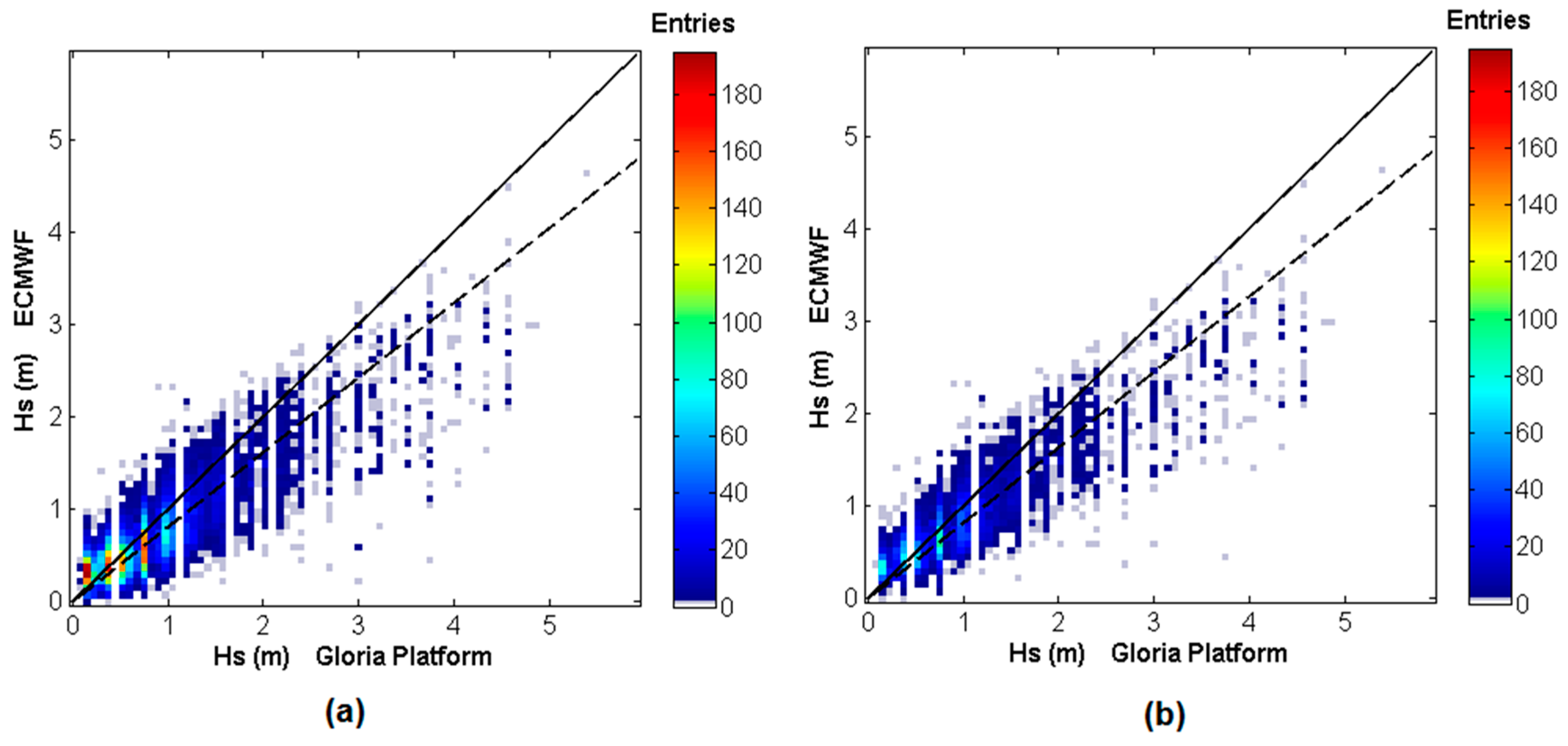
As a first step, a direct comparison will be carried out between the in situ measurements coming from the Gloria drilling platform and the ECMWF data reported for this site. The results are indicated for the interval 2003–2009, being reported in terms of the following statistical index: (m)—average value indicated for the Gloria in situ measurements; (m)—average value indicated for the ECMWF data; Bias (m)—differences between and ; Root-Mean-Square Error (RMSE in meters)—measure of disagreement; Scatter Index (SI)—measure of the magnitude of a set of numbers (RMSE/); Pearson correlation index (R).
The corresponding scatter plots are presented in Figure 2, while a detailed statistical analysis is presented in Table 1. The Hs values registered at the Gloria station are higher than the ones indicated by the ECMWF data, revealing a bias of 0.15 m (in winter) and 0.14 m (total time), respectively. The RMSE index is frequently used to assess the differences reported between the datasets, using as a reference the zero value, which represents a perfect correlation. This is not the case, however; a maximum value of 0.44 m was reported for the winter time compared to 0.40 m indicated for the total time. For the considered time interval the SI presents values in the range 0.39–0.43, while the R index is located close to the value of 0.9.
2.3. The AVISO Satellite Measurements
Maybe the best way to identify the natural conditions of the vast marine areas is through satellite missions. Compared to a fixed in situ station, the benefit of an altimeter mission is that it can cover an extended area, while the drawback is that the results are available only for the satellite track; even so, this can be compensated for by combining data from multiple missions. The principles behind the measurements of the wave heights are relatively simple, involving a radar pulse sent by the altimeter to the rough sea surface. The beam energy reflected by the water surfaces is received by the satellite, and in this way it is possible to determine the wave profile based on the waveform and the amplitude of the return signal. In the case of coastal waters, it is possible that the altimeter signal can be contaminated by land if we take into account the size of the antenna footprint [34]. The AVISO (Archiving, Validation, and Interpretation of Satellite Oceanographic Data) project, initially started in 1986, was considered an important source of high-quality altimeter data. From the past missions there can be mentioned Geosat, ERS-1, Topex/Poseidon, Envisat, or Jason-1, while during the present day the following missions are active: Sentinel-3, Jason-3, Saral, HY-2, Cryosat, and Jason-2 [35]. All these measurements are inter-calibrated and merged, being assembled in a single global dataset.
In the AVISO project there are included all the altimeter missions designed to operate on repeated tracks and geodetic orbits. For example, the mission Jason-1 follows a 10-day exact repeat cycle; mission ERS-1 was defined by a repeat 35-day and geodetic 168-day period orbits, while the CryoSat mission is defined by a repeat period of 369 days—5344 revolutions (30 day sub-cycle) [36,37,38]. These measurements are processed through the DUACS (Data Unification and Altimeter Combination System) platform, which is a component of the CNES multi-mission ground segment (SSALTO). In order to assemble a database, the initial measurements are processed in various sequences, which involve: acquisition, homogenization, input data quality control, multi-mission cross-calibration, product generation, merging, and final quality control. During these steps specific algorithms are applied and the multi-satellite orbit error reduction is computed or a gridded product is generated [39]. For the Black Sea area, the AVISO wave data will be used, covering the interval 2010–2016, with the available dataset defined by a single measurement per day (00 UTC).
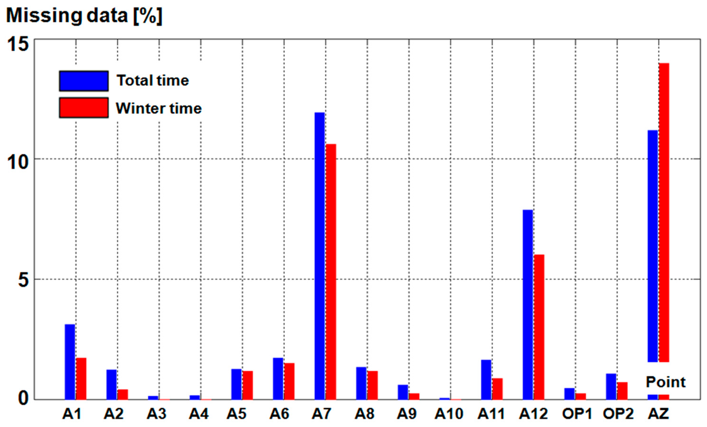
An import aspect related to the satellite missions is the presence of missing values, which represent gaps in the time series denoted with NaN (Not a Number) [40]. A quality check is carried out in Figure 3 for all the reference points, taking into account the total and winter time intervals. In general, most of the values are located below the 5% limit, with a more consistent distribution noticed during the total time interval.
A much higher value is indicated for point A12, which indicates7.86% (total time) and 6.01% (in winter), while points A7 and AZ exceed the 10% limit, reaching a maximum of 13.98% (AZ in winter). As expected, the quality of the results is influenced by the missing values and in general it is recommended that the NaN percentage does not exceed 10% of the total value [41]. Therefore, in the case of points A7 and AZ the satellite measurements represent a viable instrument to monitor these areas.
3. Results
3.1. Evaluation of the ECMWF Data
In order to assess the long-term variations in Black Sea wave conditions, the 38 years of ECMWF data (1979–2016) will be considered for evaluation.
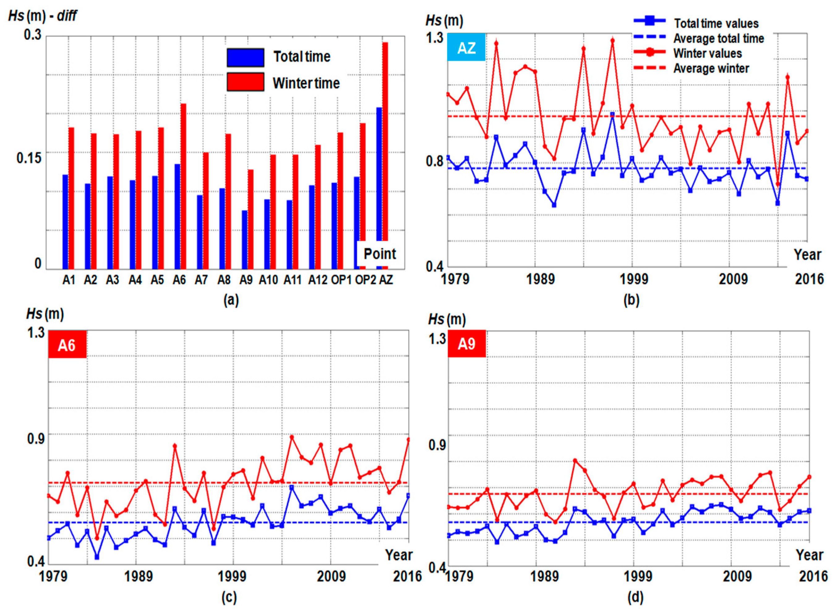
Figure 4 illustrates the distribution of the mean values reported on inter-annual scale for various time intervals (total and winter time). Figure 4a presents the differences reported between the maximum and minimum annual values, corresponding to the interval 1979–2016. Excepting points AZ and A6, most of the variations are located below 0.2 m, with reference point A6 exceeding these limits only during the winter. On the opposite end, point A9 presents a minimum of 0.07 (total time) compared to 0.12 m reported in winter. The group points A1–A5 (located in the north) present smaller variations, indicating values of 0.10–0.12 m (total time) and 0.17–0.18 m (in winter), respectively. Also, there is a gradual increase in the differences from point A9 (Turkey) to A12 (Bulgaria) and A1 (Romania), which, for example, during the winter starts at 0.12 m and finally reaches 0.18 m (in A1).
Since points A6, AZ, and A9 are more representative in terms of these variations, Figure 4b–d represent the mean annual values while with a dotted line that indicates the absolute average for this time interval.
The winter season is more variable, as can be observed in the case of the site AZ, where the values are in the range 0.71–1.27 m. During the interval 1979–1999 most of the values exceeded the absolute averages, which are set to 0.77 m (total time) and 0.98 m (in winter), and during recent years (2010–2011) there is a tendency of the Hs values to exceed these limits. In the case of point A6, it can be observed that the maximum values are located in the interval 1990–2016, and may reach 0.69 m (total time) and 0.89 m (winter), both being reported for 2004. Regarding point A9, which is located in the southern area, a maximum peak of 0.8 m is seen in 1992, while in 1999 the values largely exceeded the absolute mean.
In order to avoid the influence of outliers, in Figure 5 the 95 percentile index was considered in the identification of the maximum annual significant wave heights for all the points, which were grouped according to the reference sector. Since during the winter season the highest values are reported, only this period was taken into account. The points located in areas I, II, and IV present maximum values of 3.3 m, 3.5 m, and 3 m, respectively, for 1993, compared to area III, where a 2.4 m value is indicated for 1987.
From the points located in area I, it can be noticed that sites A1 and A3 present in general much higher values compared to point A2, where the values are located in the range 1.66–2.68 m. As expected, the offshore points OP1 and OP2 present more important values, which are located in the range 1.6–2.37 m and 2–3 m, while for the Azov Sea a minimum of 1.64 m was reported.
Figure 6 illustrates the monthly distribution of the differences reported between the minimum and maximum average values for 1979–2016. Although the winter is considered to be more dynamic, the differences between the summer and winter are not clearly highlighted by the results. For sector I, during January and March maximum variations may occur of 1.23 m, especially in the case of points A1 and A3, while during August point A1 presents a peak value of 1.11 m. Significantly lower variations are reported in June, where a minimum of 0.65 m is indicated in the vicinity of reference point A2. The points located in sector II are in general dominated by the values reported by point AZ, which during the interval June–September may reach a variation of 1.58 m. This easily exceeds the winter values, defined by a maximum of 1.17 m (point A4). In the case of sectors III and IV, the offshore points OP1 and OP2 report the highest values, indicating a value of 1.27 m for OP1 (in January) and 1.01 m for OP2 (in July). It can be observed that during July there is a peak, which modified the monthly pattern. In the case of sector IV this is defined by the following trends: A4—lower values; A5—values > A4; A6—values > A4 and A5.
One way to estimate the sea state is through the Beaufort scale, which was introduced in 1807 by Francis Beaufort. The scale is divided into 12 classes, starting from C1 (calm) and reaching hurricane conditions, during which wind speeds of 32.7 m/s can be encountered [42,43]. According to the values defined in this scale, three sea state conditions were defined for the present study: (A) Calm sea state (C) → Hs ≤ 0.6 m; (B) Moderate sea state (M) → 0.6 m < Hs ≤ 2.5 m; (C) Rough sea state (R) → Hs > 2.5 m.
Table 2 presents the distribution of the three classes (in %) for various time intervals, from which it can be seen that point A7 can be associated with the values reported in the calm area, compared to point OP1, which registers significant values from the moderate and rough classes. The three main time intervals (1979–1990, 1991–2000, and 2001–2016) reveal the following general trends: (A) Calm values—decreases to the second interval and increases for the third; (B) and (C) Moderate and rough values—increases to the second interval and decreases to the third.
In terms of the calm values, the maximum of 77.83% is accounted for by point A7 during 1979–1990, compared to a minimum of 25.48% indicated by OP1 for 1991–2000. For moderate conditions, there are values in the range 69.61–71.84% for points A3 and OP1 for 1991–2000,downto a minimum of 22.08% reported by A7 in the interval 1979–1990. A maximum of 2.74% and 2.78% is reported for the rough classes by the reference points OP1 and AZ, respectively.
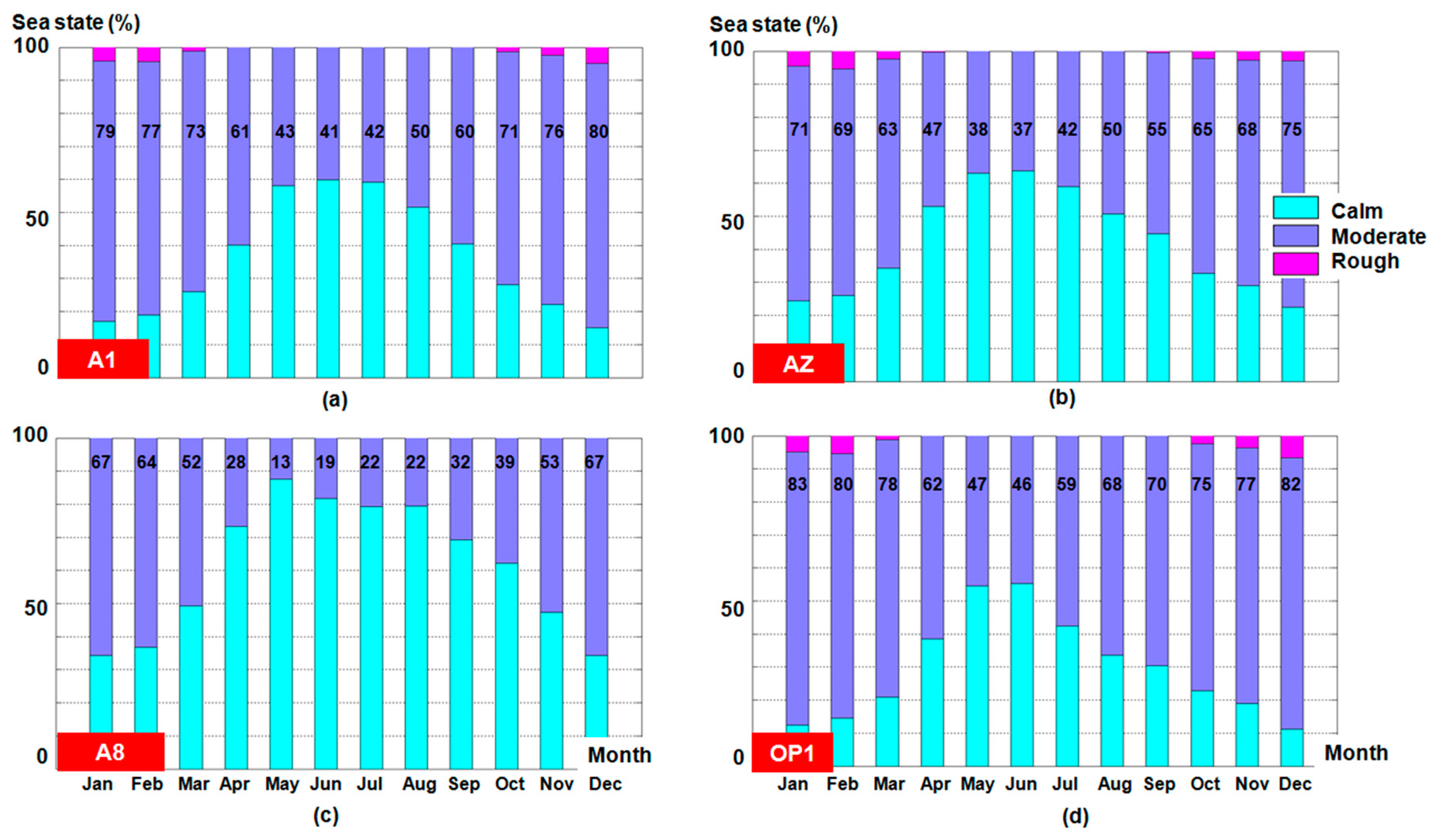
A similar analysis is presented in Figure 7 for several reference points, with the monthly distribution taken into account this time. The presence of the summer season (April–September) is clearly highlighted by the values from the calm interval, while the rough conditions are briefly noticed during the winter, though site A8 does not report such events. In the case of point A1, moderate conditions may be present during the summer (values in the range of 41–61%), compared to the winter, when these values increase to 71–80%.
For the same classes, point A8 presents a minimum of 13% in May, and maximum of 64–67% during December–February. In the case of the offshore point OP1, the rough conditions may reach a maximum of 4.5–7.28% during the interval November–February, while in March and October the extreme events do not exceed 3.47%. Finally, during the summer these conditions account for a maximum of 1% of the total values.
3.2. Assessment of the AVISO Measurements
Table 3 presents a statistical evaluation of the Hs values reported during the total and winter time, respectively. In terms of average values, the differences between the reference points are much smaller. Thus, during the total time these differences may reach a maximum around 0.9 m, compared to AZ, which this time presents a much smaller value of 0.76 m. During the winter, these values are distributed around the value of 1 m, with more noticeable conditions being accounted for by the group points A10–A12 and by point OP1. The values reported by the 95 percentile are half those of the extreme ones (indicated throughout by the subscript Max).
A more severe difference is reported by point A7, where the maximum is 6.57 m compared to 1.81 m accounted for by the percentile. The distribution of calm, moderate, and rough conditions is also presented, with the rough values reported by the AVISO measurements for point AZ being much smaller than the ones reported by the ECMWF data.
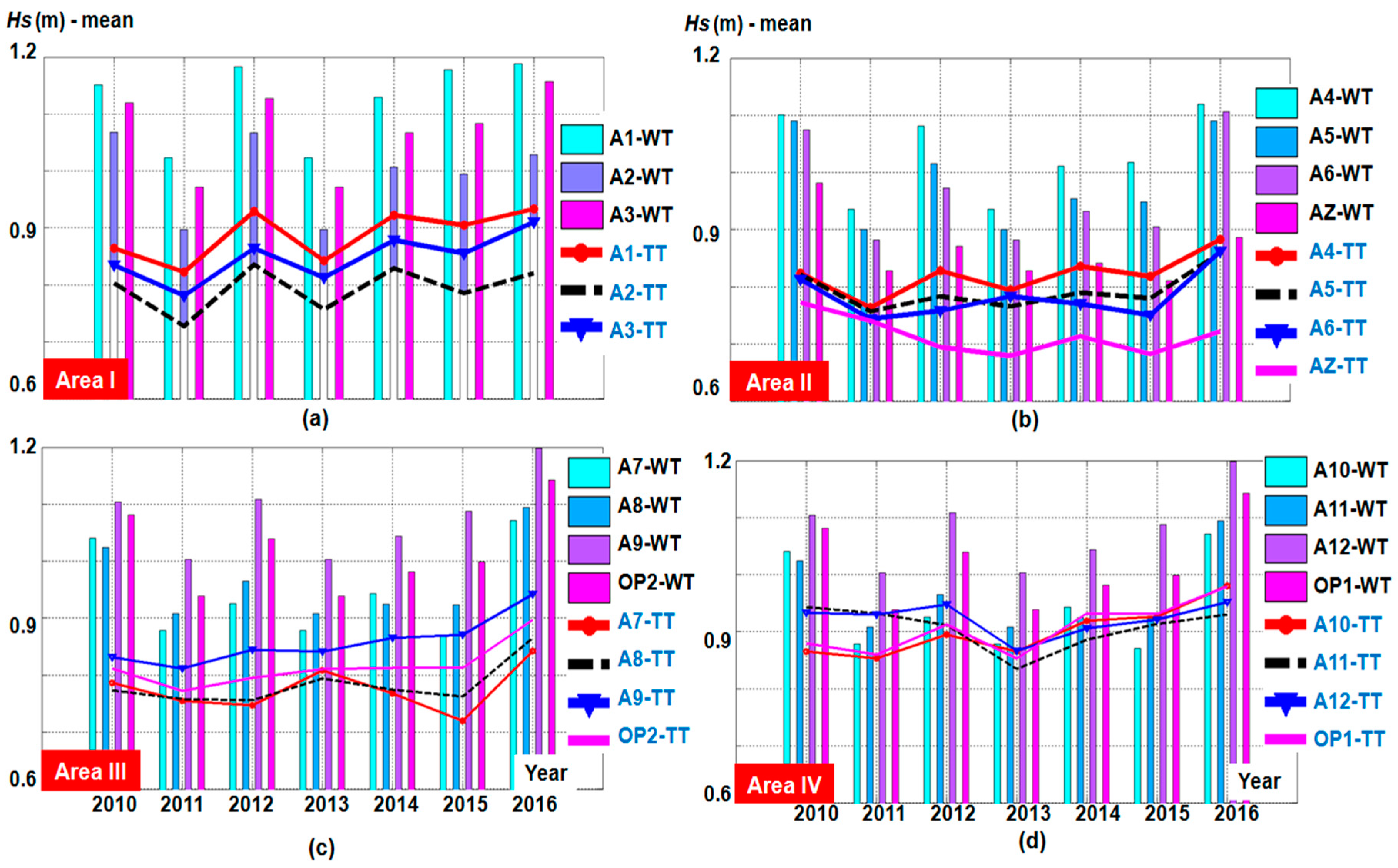
The distribution of the mean values on an annual scale is presented in Figure 8, considering all the reference points. In general, sites A1, A3–A5, A9, A12, OP1, and OP2 present much higher values, and some seasonal trends have also been reported. During 2011 and 2013 lower values are reported compared to 2010 and 2012, while during the interval 2014–2016 the wave heights are slowly increasing until they reach a maximum in 2016. The following results can be mentioned: (A) Sector I—point A1→ 1.18 m in 2012 and 2016; (B) Sector II—A4 →1.12 m in 2016; (C) Sector III/IV—A9 and A12→ 1.2 m in 2016.
Figure 9 illustrates the annual distribution of the extreme Hs values, from which it can be observed that 2012 presents some energetic peaks, such as: A1—5.6 m; A4—4.39 m; A11 and A12—5.55 m, in contrast with sector III, where point A7 presents a maximum of 6.57 m in 2010. In general, the values reported in sectors I and IV are located below the 4 m limit, a minimum of 2.4 m being accounted for by point A3. For sectors II and III, the annual values do not exceed 3.5 m, excepting point A9, which has two peaks at4.18 m (in 2012) and 3.63 m (in 2014), respectively.
The monthly sea state distribution illustrated by the satellite measurements is presented in Figure 10. By adding up the calm, moderate, and rough values, we can obtain a complete overview of the sea state (100%), but in the case of the satellite data there is a problem associated with the missing values, also known as NaN—Not a Number [44]. As can be observed, some points present no gaps in the time series, such as in the case of A3, A10, or OP1 compared to AZ or A7, an aspect that can be observed in Table 3. During the winter, and also during April, August, and September, the values from the moderate classes are dominant compared to the remaining months, when the heights from the calm interval start to gain momentum.
The rough conditions are visible only during the winter; the month of December is most variable from this point of view, with values of A1—5%, A3 and A9—4.07%, A10—5.88%, A11 and OP1—6.33%. For point AZ, there is a tendency to have missing data in the interval January–April, when the following percentages are reported: January—18.84%, February—27.8%, March—17%, and April—12%. Since the Azov Sea is a relatively small area compared to the Black Sea, these gaps can be considered a weak point of the satellite measurements, including in this category the costal sectors defined by a complex orography, such as points A7 or A12. Most of the points follow a similar pattern, which, for example, in the case of A1 is defined by an 87.6% of Hs values from the moderate interval (in January), which drops to 45.4% in July. Of the offshore points, site OP1 seems to be more dynamic, indicating during June and July calm values that register a maximum of 47.1% compared to OP2, where a value of 52.9% is noticed.
4. Discussion
A first analysis is carried out in Figure 11 for the ECMWF data, where the results are presented in descending order, being based only on the total time values. Regarding the mean values (Figure 11a), the top four points are OP1, A3, A4, and A1, with Hs values exceeding 0.8 m. Close behind is point AZ (from the Azov Sea), located at0.78 m, which exceeds the offshore point OP2 by only 0.71 m. On an opposite end, we found the group points A6–A9, which present values in the range 0.42–0.57 m, much lower, being registered in the vicinity of site A7, which is located in the eastern side of the sea. Regarding the 95th percentile, it can be observed that the first position is occupied by points OP1, A3, A4, and A1, and at this time point AZ with 2.02 m exceeds point A1, which indicates a value of 1.97 m. On the other hand, we found the same group points A6–A9, which present a maximum of 1.46 m and a minimum of 1.03 m.
Although point OP2 is located offshore, at 1.69 m, this confirms the fact that the eastern part of the Black Sea is defined by a lower wave energy level compared to the western one. In terms of the calm conditions (in %), in first place we find the group points A6–A12 located in the northeast and northern sectors, which present a minimum of 48% for A12 and a maximum of 73% for site A7. Much lower values are accounted for by the group points A1–A4, with a maximum of 39.7%, while a minimum of 29.7% is reported close to point OP1. The rough conditions, as reported by the ECMWF dataset, do not exceed 3% of the total time, being located between a maximum of 2.63% for OP1 and ≈0% for point A8. Based on these results, three main groups of points can be highlighted, namely: (A) OP1, A3, AZ, A4, and A1 with values in the range of 2.06–2.63%; (B) A5, A12, A2, OP2, and A11 with values in the range of 0.78–1.52 m; (C) A10, A6, A9, A7, and A8 with values in the range of 0.07–0.39%.
Some insights regarding the temporal and spatial variations of the wave conditions are illustrated in Figure 12 through the AVISO measurements.
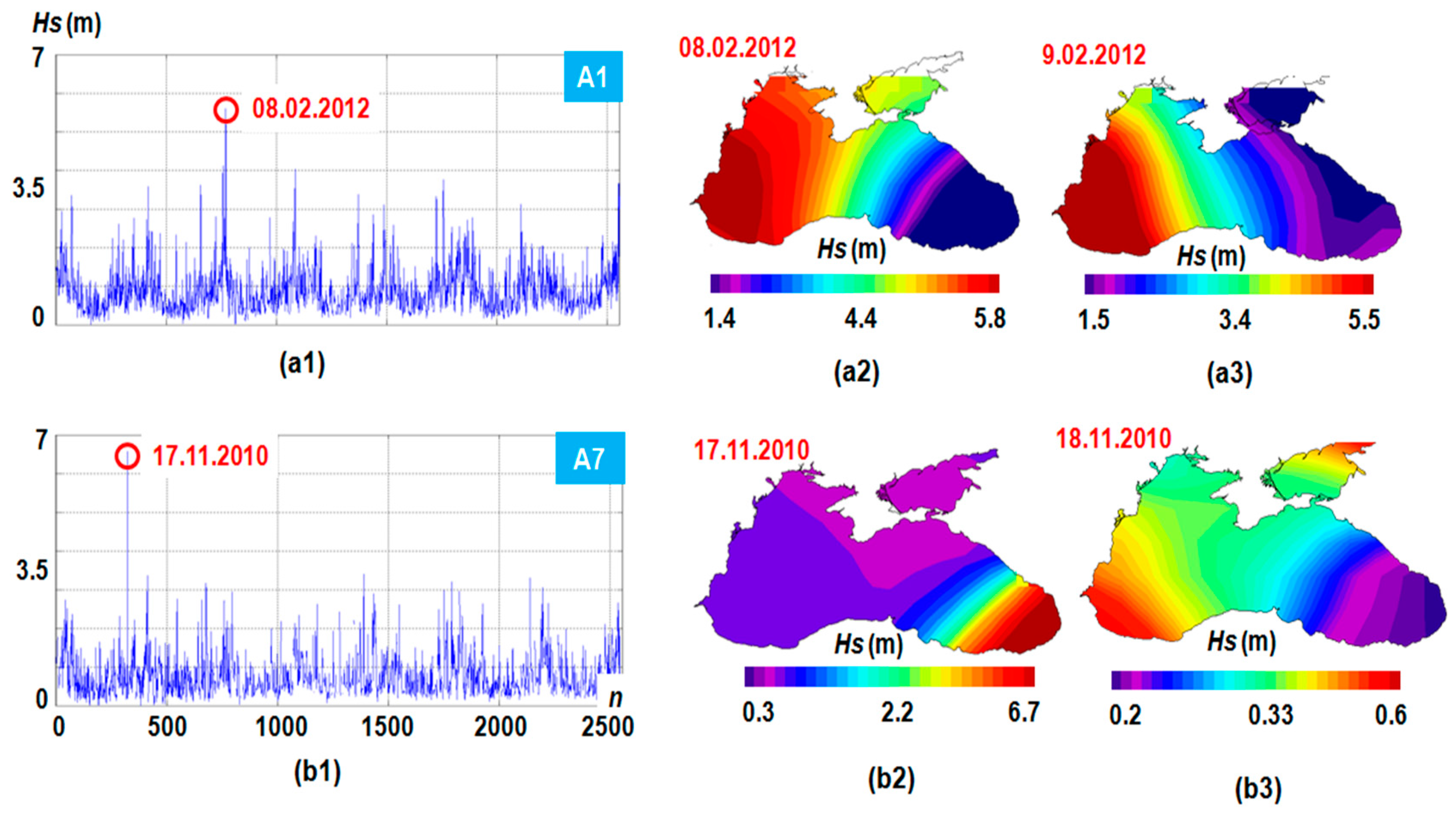
In order to highlight the distribution of the storm events in the Black Sea region, the time series of points A1 and A7 were considered for evaluation and to identify some energetic peaks. For point A1 a major event is reported for 8 February 2012, during which a maximum of 5.8 m may be observed in the western part of the sea, while a minimum of 1.4 m was reported in the eastern sector. According to the values reported during the next day, the peak of the storm is gradually moving to the southwest, while in the middle of the basin and in the Azov Sea there are reported Hs values from the lower classes. Regarding point A7, located in the eastern sector, a maximum peak of 6.7 m was observed on17 November 2010. In this case, most of the Black Sea areas present calm conditions, with the storm being concentrated in the vicinity of the Georgian nearshore. On the next day, the spatial distribution of the wave conditions had completely changed, with in this case more important values being reported in the southwest sector (0.6 m) compared to a minimum of 0.2 m reported in the southeast.
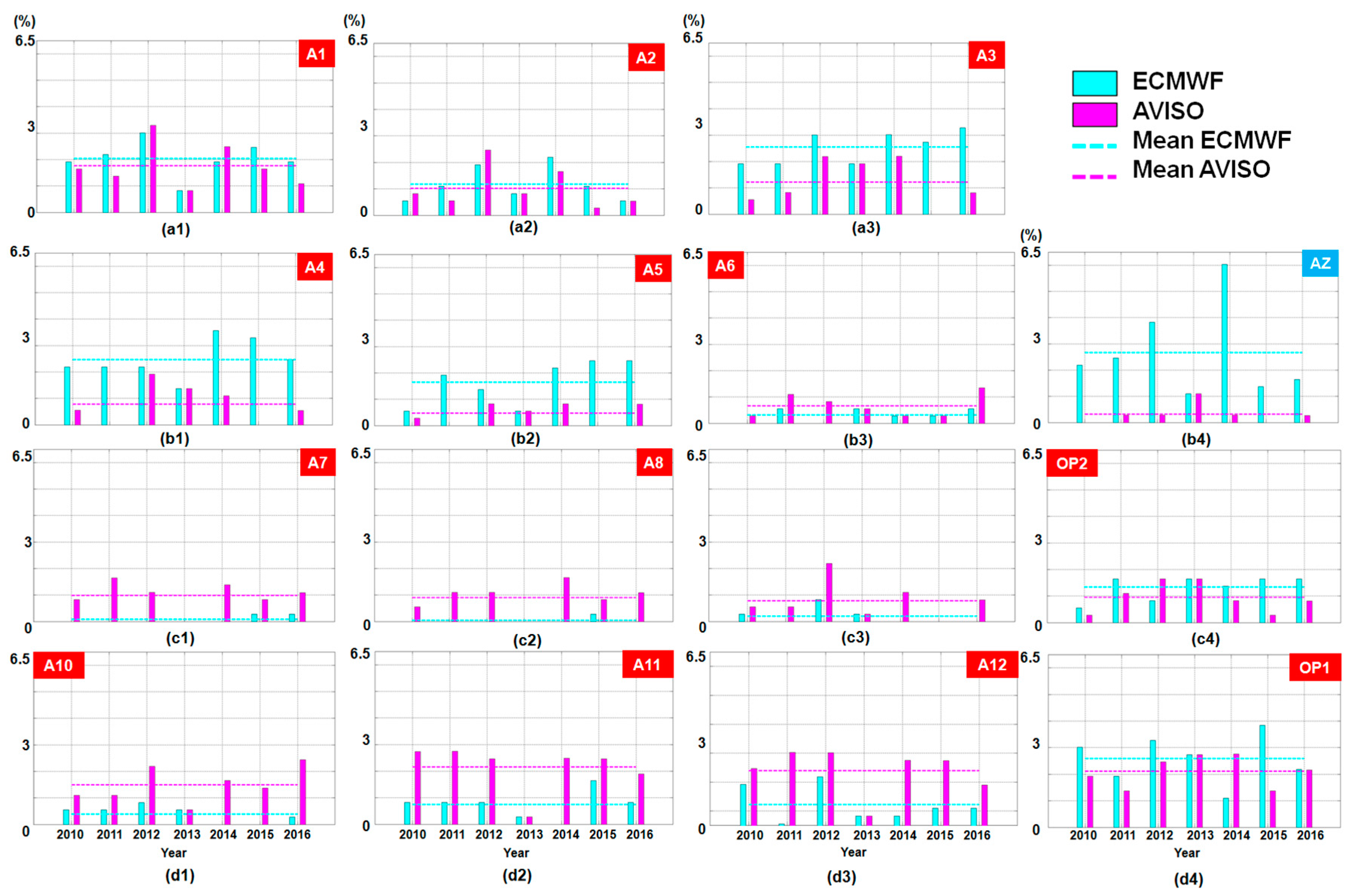
Since rough conditions represent a real threat to offshore and coastal activities, in Figure 13 a joint evaluation of the annual events reported by the ECMWF and AVISO datasets for the interval 2010–2016is carried out. The differences between the two datasets are obvious, with no rough conditions being reported group points A7–A9 according to the ECMWF data. In general, the annual values are located below the mean values, excepting points A11 and A12, which, based on the AVISO data, present a maximum of five years above this value.
Most of the points present values below 2.5%, with a maximum peak of 6.03% (in 2014) also being reported for point AZ according to the ECMWF data. For the AVISO measurements, a maximum of 3.29% was seen in the case of point A1, which corresponds to 2012. For points located in sector I, there is a tendency of the ECMWF values to report higher values, excepting points A1 (2012 and 2014) and A2 (2012), where the AVISO shows more consistent results. Regarding points from sector II, the ECMWF values are dominant, excepting site A6, where the reverse trend is observed. Regarding the offshore points, the rough conditions reported by the AVISO data are, in general, smaller, though in 2013 there seems to be good agreement between the two datasets, which is also highlighted by the rest of the points.
5. Conclusions
In the current work, a complete picture of the Black Sea wave variability is illustrated by using both ECMWF reanalysis data and satellite measurements, considering values reported over the last 38 years (1979–2016). As a first step, a quality assessment of the selected dataset was carried out, starting with the ECMWF data, which were compared with in situ measurements coming from the Gloria drilling platform. According to this evaluation, it seems that the two datasets are in very good agreement, with a Pearson index of 0.86, which is close to an ideal positive correlation.
For the AVISO measurements, it was considered important to identify the presence of the missing values (NaN) and based on this analysis it was highlighted that points A7 and AZ may present problems from this point of view.
According to the ECMWF data, it was noticed that the differences reported on an inter-annual scale tend to increase slightly from the southern part of the sea to the southwestern sector. From this point of view, site AZ presents the highest variations, indicating a maximum of 0.3 m during the winter. In the case of reference point AZ, it can be observed that in the period 1979–1999 the Hs values in general exceeded the average value, while the opposite trend was reported after this period. If we consider the average values as a reference, we see that at points A6 and A9 there is a constant increase in the Hs values, with this tendency being more visible in 1999–2016.
From the analysis of the sea states it can be observed that in general for group points A6–A10 calm conditions are dominant, compared with the rest of the points, where moderate conditions are more frequent. If we consider only 1991–2000 we notice that the values reported in the moderate interval are more important, with a small increase in rough values also being indicated.
As to the satellite measurements, there is no correlation between the water depth and the wave resources, with more consistent values being reported in the western part of the basin. For example, point A1, located at a water depth of 41 m, presents for the total time an average value of 0.86 m, exceeding points located in deeper areas such as A4 (1995 m), A7 (1044 m), or A8 (1422). With a lower water depth and relevant wave resources, the western part of this basin may be considered a suitable candidate for a marine renewable project. In terms of the maximum values, it seems that during 2012 there were more energetic peaks in areas I, II, and IV, while a constant distribution was noticed in area III, excepting the year 2010, when there was a peak. Regarding the spatial distribution of the extreme events, it seems that the storm conditions occurring in the western part are more consistent, while in the eastern sector it is more likely to encounter storm conditions reported for a relatively short time window.
Based on these results, we can conclude that the Black Sea is a dynamic environment where the wave energy budget changes on a seasonal or inter-annual scale. These variations bring opportunities but also challenges, such as i beach erosion due to wave action. Nevertheless, for navigation and offshore activities, more important are the occurrences of rough events, which influence in a negative way the safety and productivity of these sectors.
Acknowledgments
This work was carried out in the framework of the project ACCWA (Assessment of the Climate Change effects on the WAve conditions in the Black Sea), supported by the Romanian Executive Agency for Higher Education, Research, Development and Innovation Funding—UEFISCDI, grant number PN-III-P4-ID-PCE-2016-0028. The ERA Interim data used in this study have been obtained from the ECMWF data server. The altimeter products were generated and distributed by Aviso (http://www.aviso.altimetry.fr/) as part of the Ssalto ground processing segment. The wave data corresponding to the Gloria drilling platform were provided by the National Institute for Marine Research and Development “Grigore Antipa” Constanta, Romania. Finally, the authors would like to express their gratitude to the reviewers for their constructive suggestions and observations that helped in improving the present work.
Author Contributions
Florin Onea has done the literature review and also gathered, processed, and analyzed the data. Liliana Rusu has guided this research, discussed the data, and drawn the main conclusions. The final manuscript has been approved by all authors.
Conflicts of Interest
The authors declare no conflict of interest.
Nomenclature
| ACCWA | Assessment of the Climate Change effects on the WAve conditions in the Black Sea |
| DUACS | Data Unification and Altimeter Combination System |
| ECMWF | European Center for Medium-Range Weather Forecasts |
| AVISO | Archiving, Validation and Interpretation of Satellite Oceanographic |
| ERS | European Remote Sensing |
| Hs | significant wave height |
| NaN | Not a Number |
| NOAA | National Oceanic and Atmospheric Administration |
| R | Pearson correlation index |
| RMSE | Root-Mean-Square Error |
| SAR | Synthetic Aperture Radar |
| SI | Scatter Index |
| UTC | Coordinated Universal Time |
| WAM | WAve Model |
References
- National Academy of Sciences (NAS). Climate Change Evidence & Causes; National Academies Press: Washington, DC, USA, 2014. [Google Scholar] [CrossRef]
- BBao, B.; Ren, G. Climatological characteristics and long-term change of SST over the marginal seas of China. Cont. Shelf Res. 2014, 77, 96–106. [Google Scholar] [CrossRef]
- Makris, C.P.; Galiatsatou, C.P.; Tolika, K.; Anagnostopoulou, C.; Kombiadou, K.; Prinos, P.; Velikou, K.; Kapelonis, Z.; Tragou, E.; Androulidakis, Y.; et al. Climate change effects on the marine characteristics of the Aegean and Ionian Seas. Ocean Dyn. 2016, 66, 1603–1635. [Google Scholar] [CrossRef]
- McTaggart-Cowan, R.; Bosart, L.F.; Gyakum, J.R.; Atallah, E.H. Hurricane Katrina (2005). Part I: Complex life cycle of an intense tropical cyclone. Mon. Weather Rev. 2007, 135, 3905–3926. [Google Scholar] [CrossRef]
- Le Roy, S.; Pedreros, R.; André, C.; Paris, F.; Lecacheux, S.; Marche, F.; Vinchon, C. Coastal flooding of urban areas by overtopping: Dynamic modeling application to the Johanna storm (2008) in Gâvres (France). Nat. Hazards Earth Syst. Sci. 2015, 15, 2497–2510. [Google Scholar] [CrossRef] [Green Version]
- Rusu, E.; Onea, F. Study on the influence of the distance to shore for a wave energy farm operating in the central part of the Portuguese nearshore. Energy Conver. Manag. 2016, 114, 209–223. [Google Scholar] [CrossRef]
- Onea, F.; Rusu, E. The expected efficiency and coastal impact of a hybrid energy farm operating in the Portuguese nearshore. Energy 2016, 97, 411–423. [Google Scholar] [CrossRef]
- Onea, F.; Rusu, L. Coastal impact of a hybrid marine farm operating close to the Sardinia Island. In Proceedings of the OCEANS’15 MTS/IEEE, Genova, Italy, 18–21 May 2015. [Google Scholar] [CrossRef]
- Krasnopolsky, V.; Nadiga, S.; Mehra, A.; Bayler, E.; Behringer, D. Neural networks technique for filling gaps in satellite measurements: Application to ocean color observations. Comput. Intell. Neurosci. 2016, 2016. [Google Scholar] [CrossRef] [PubMed]
- Dee, D.P.; Uppala, S.M.; Simmons, A.J.; Berrisford, P.; Polim, P.; Kobayashi, S.; Andrae, U.; Balmaseda, M.A.; Balsamo, G.; Bauer, P.; et al. The ERA-Interim reanalysis: Configuration and performance of the data assimilation system. Q. J. R. Meteorol. Soc. 2011, 137, 553–597. [Google Scholar] [CrossRef]
- Peres, D.J.; Iuppa, C.; Cavallaro, L.; Cancelliere, A.; Foti, E. Significant wave height record extension by neural networks and reanalysis wind data. Ocean Model. 2015, 94, 128–140. [Google Scholar] [CrossRef]
- Caires, S.; Sterl, A. Comparative assessment of ERA-40 ocean wave data. In Proceedings of the ECMWF Workshop on Re-Analysis, Reading, UK, 5–9 November 2001; pp. 353–368. [Google Scholar]
- Volkov, D.L.; Landerer, F.W. Internal and external forcing of sea level variability in the Black Sea. Clim. Dyn. 2015, 45, 2633–2646. [Google Scholar] [CrossRef]
- Yarovaya, D.A. Intense Mesocyclones in the Black Sea Region. Russ. Meteorol. Hydrol. 2016, 41, 535–543. [Google Scholar] [CrossRef]
- Yarovaya, D.A.; Efimov, V.V. Mesoscale Cyclones over the Black Sea. Russ. Meteorol. Hydrol. 2014, 39, 378–386. [Google Scholar] [CrossRef]
- Efimov, V.V.; Krupin, A.V. Breeze Circulation in the Black Sea Region. Russ. Meteorol. Hydrol. 2016, 41, 240–246. [Google Scholar] [CrossRef]
- Onea, F.; Raileanu, A.; Rusu, E. Evaluation of the wind energy potential in the coastal environment of two enclosed seas. Adv. Meteorol. 2015, 14. [Google Scholar] [CrossRef]
- Onea, F.; Rusu, E. Wind energy assessments along the Black Sea basin. Meteorol. Appl. 2014, 21, 316–329. [Google Scholar] [CrossRef]
- Raileanu, A.; Rusu, L.; Rusu, E. Wave modelling with data assimilation in the Romanian nearshore. In Proceedings of the 16th International Congress of the International Maritime Association of the Mediterranean, IMAM Towards Green Marine Technology and Transport, Pula, Croatia, 21–24 September 2015; pp. 837–843. [Google Scholar] [CrossRef]
- Rusu, L. Assessment of the wave energy in the Black Sea based on a 15-year hindcast with data assimilation. Energies 2015, 8, 10370–10388. [Google Scholar] [CrossRef]
- Gasparotti, C.; Rusu, E. Methods for the risk assessment in maritime transportation in the Black Sea basin. J. Environ. Prot. Ecol. 2012, 13, 1751–1759. [Google Scholar]
- Rusu, L.; Butunoiu, D.; Rusu, E. Analysis of the extreme storm events in the Black Sea considering the results of a ten-year wave hindcast. J. Environ. Prot. Ecol. 2014, 15, 445–454. [Google Scholar]
- Aydogan, B.; Ayat, B.; Yüksel, Y. Black Sea wave energy atlas from 13 years hindcasted wave data. Renew. Energy 2013, 57, 436–447. [Google Scholar] [CrossRef]
- Rusu, L.; Bernardino, M.; GuedesSoares, C. Wind and wave modelling in the Black Sea. J. Oper. Oceanogr. 2014, 7, 5–20. [Google Scholar] [CrossRef]
- Zanopol, A.T.; Onea, F.; Rusu, E. Coastal impact assessment of a generic wave farm operating in the Romanian nearshore. Energy 2014, 72, 652–670. [Google Scholar] [CrossRef]
- Rusu, E.; Onea, F.; Toderascu, R. Dynamics of the environmental matrix in the Black Sea as reflected by recent measurements and simulations with numerical models. In The Black Sea: Dynamics, Ecology and Conservation; Nova Science Publishers: New York, NY, USA, 2011; ISBN 978-1-61324-742-6. [Google Scholar]
- Onea, F.; Rusu, E. An evaluation of the wind energy in the North-West of the Black Sea. Int. J. Green Energy 2014, 11, 465–487. [Google Scholar] [CrossRef]
- Pastor, J.; Liu, Y.C. Wave climate resource analysis for deployment of wave energy conversion technology. Sustainability 2016, 8, 1321. [Google Scholar] [CrossRef]
- Pastor, J.; Liu, Y.; Dou, Y. Wave energy resource analysis for use in wave energy conversion. In Proceedings of the Industrial Energy Technology Conference (IETC 2014), New Orleans, LA, USA, 20–23 May 2014. [Google Scholar]
- Iuppa, C.; Cavallaro, L.; Vicinanza, D.; Foti, E. Investigation of suitable sites for wave energy converters around Sicily (Italy). Ocean Sci. 2015, 11, 543–557. [Google Scholar] [CrossRef]
- European Centre for Medium-Range Weather Forecasts (ECMWF). IFS Documentation—Cy31r1, Operational Implementation. Part VII: ECMWF Wave Mode; European Centre for Medium-Range Weather Forecasts: Reading, UK, 2006. [Google Scholar]
- Raileanu, A.; Onea, F.; Rusu, E. Assessment of the wind energy potential in the coastal environment of two enclosed seas. In Proceedings of the OCEANS’15 MTS/IEEE, Genova, Italy, 18–21 May 2015. [Google Scholar] [CrossRef]
- Cavaleri, L. Wave modeling-missing the peaks. J. Phys. Oceanogr. 2009, 39, 2757–2778. [Google Scholar] [CrossRef]
- Sepulveda, H.H.; Queffeulou, P.; Ardhuin, F. Assessment of SARAL AltiKa wave height measurements relative to buoy, Jason-2 and Cryosat-2 data. Mar. Geod. 2015, 38, 449–465. [Google Scholar] [CrossRef]
- Archiving, Validation and Interpretation of Satellite Oceanographic Data (AVISO). 2017. Available online: http://www.aviso.altimetry.fr/ (accessed on 10 August 2017).
- CNES (Centre National d’Etudes Spatiales). Jason-1 Products Handbook; Centre National d’Etudes Spatiales: Paris, France, 2016; Volume 5. [Google Scholar]
- Pujol, M.I.; Faugère, Y.; Taburet, G.; Dupuy, S.; Pelloquin, C.; Ablain, M.; Picot, N. DUACS DT2014: The new multi-mission altimeter data set reprocessed over 20 years. Ocean Sci. 2016, 12, 1067–1090. [Google Scholar] [CrossRef]
- ESA (European Space Agency). CryoSat Mission and Data Description; European Space Agency: Paris, France, 2007. [Google Scholar]
- AVISO (Archiving, Validation and Interpretation of Satellite Oceanographic Data). SSALTO/DUACS User Handbook: MSLA and (M)ADT Near-Real Time and Delayed Time Products; Centre National d’Etudes Spatiales: Paris, France, 2016; Volume 5. [Google Scholar]
- Risien, C.M.; Chelton, D.B. A satellite-derived climatology of global ocean winds. Remote Sens. Environ. 2006, 105, 221–236. [Google Scholar] [CrossRef]
- Dong, Y.; Peng, C.Y.J. Principled missing data methods for researchers. SpringerPlus 2013, 2, 222. [Google Scholar] [CrossRef] [PubMed]
- National Meteorological Library and Archive. Fact Sheet 6—The Beaufort Scale Version 01. Available online: https://www.metoffice.gov.uk/binaries/content/assets/mohippo/pdf/b/7/fact_sheet_no._6.pdf (accessed on 20 August 2017).
- WMO (World Meteorological Organization). Manual on Codes International Codes No. 306. World Meteorological Organization: Geneva, Switzerland, 1995; Volume I.1, Part A: Alphanumeric Codes (Section E1). [Google Scholar]
- Onea, F.; Deleanu, L.; Rusu, L.; Georgescu, C. Evaluation of the wind energy potential along the Mediterranean Sea coasts. Energy Explor. Exploit. 2016, 34, 766–792. [Google Scholar] [CrossRef]
Figure 1.
Location of the reference points considered in the Black Sea area. Figure processed from Google Earth (2017). The water depths correspond to the values reported by the NOAA bathymetric database (https://maps.ngdc.noaa.gov/viewers/bathymetry/).
Figure 1.
Location of the reference points considered in the Black Sea area. Figure processed from Google Earth (2017). The water depths correspond to the values reported by the NOAA bathymetric database (https://maps.ngdc.noaa.gov/viewers/bathymetry/).
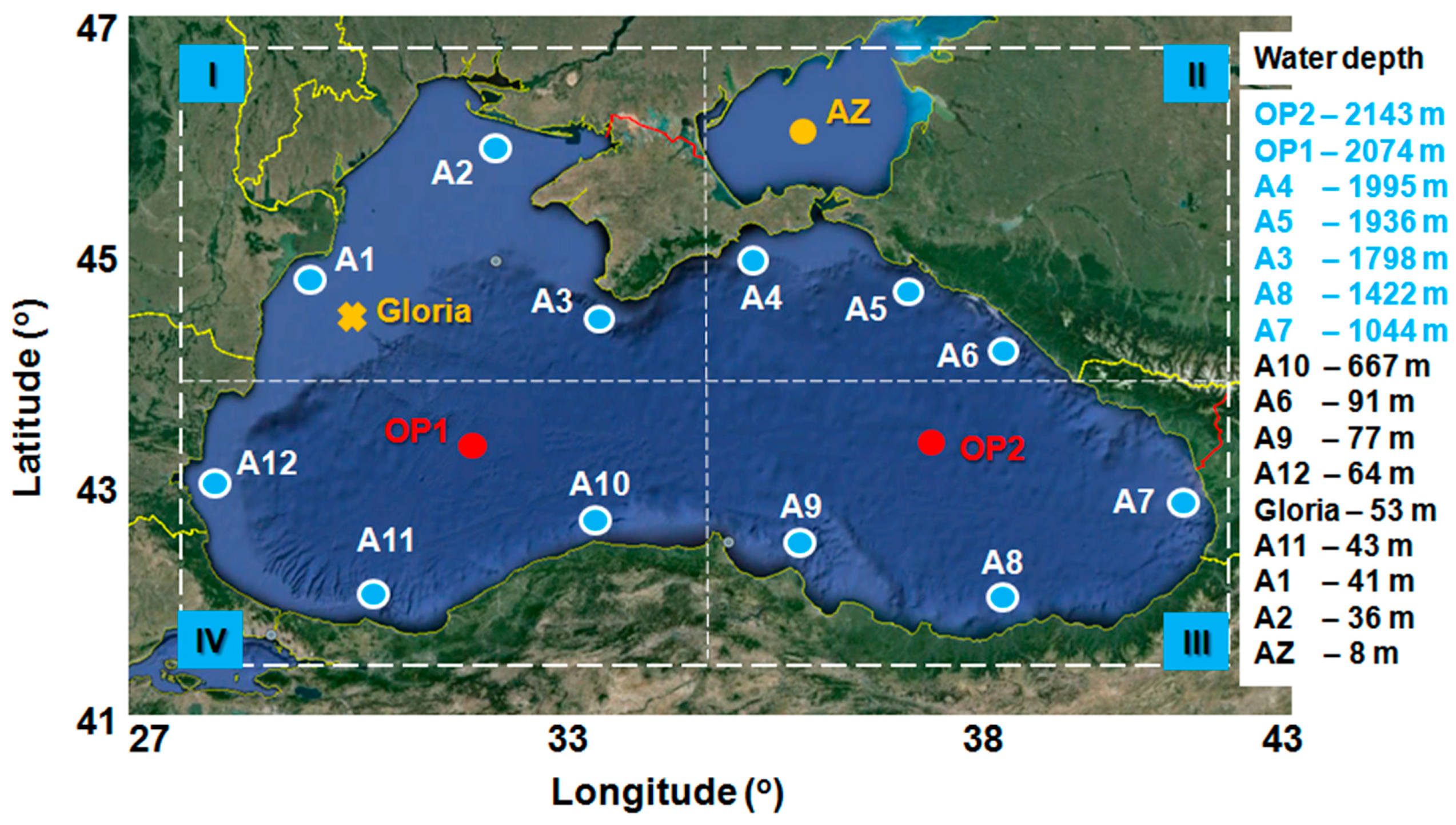
Figure 2.
Scatter diagrams of the Hs parameter corresponding to the in situ measurements (from Gloria drilling platform) and ECMWF data, considering the time interval 2003–2009: (a) total time; (b) winter time. Different colors correspond to different quantities of data in the single pixels. The solid lines denote the perfect fit to the modeled and measured values and the dashed lines represent the best-fit slope.

Figure 3.
Distribution of the missing data (NaN—not a number), corresponding to the AVISO measurements. The results are reported for the period 2010–2016, being computed for the total and winter time intervals, respectively.
Figure 3.
Distribution of the missing data (NaN—not a number), corresponding to the AVISO measurements. The results are reported for the period 2010–2016, being computed for the total and winter time intervals, respectively.

Figure 4.
Inter-annual distribution of the average values based on the ECMWF data, as indicated for the time interval 1979–2016. The results are related to: (a) normalized values reported between the maximum variation and the average value; (b–d) annual variations computed for the total and winter time, respectively, by considering points AZ, A6, and A9.

Figure 5.
Inter-annual distribution of the Hs—95 percentile values (in meters) based on the analysis of 38 years (1979–2016) of ECMWF data. The results correspond to the points located in: (a) Area I; (b) Area II; (c) Area III; (d) Area IV. Values estimated for the winter interval only.
Figure 5.
Inter-annual distribution of the Hs—95 percentile values (in meters) based on the analysis of 38 years (1979–2016) of ECMWF data. The results correspond to the points located in: (a) Area I; (b) Area II; (c) Area III; (d) Area IV. Values estimated for the winter interval only.
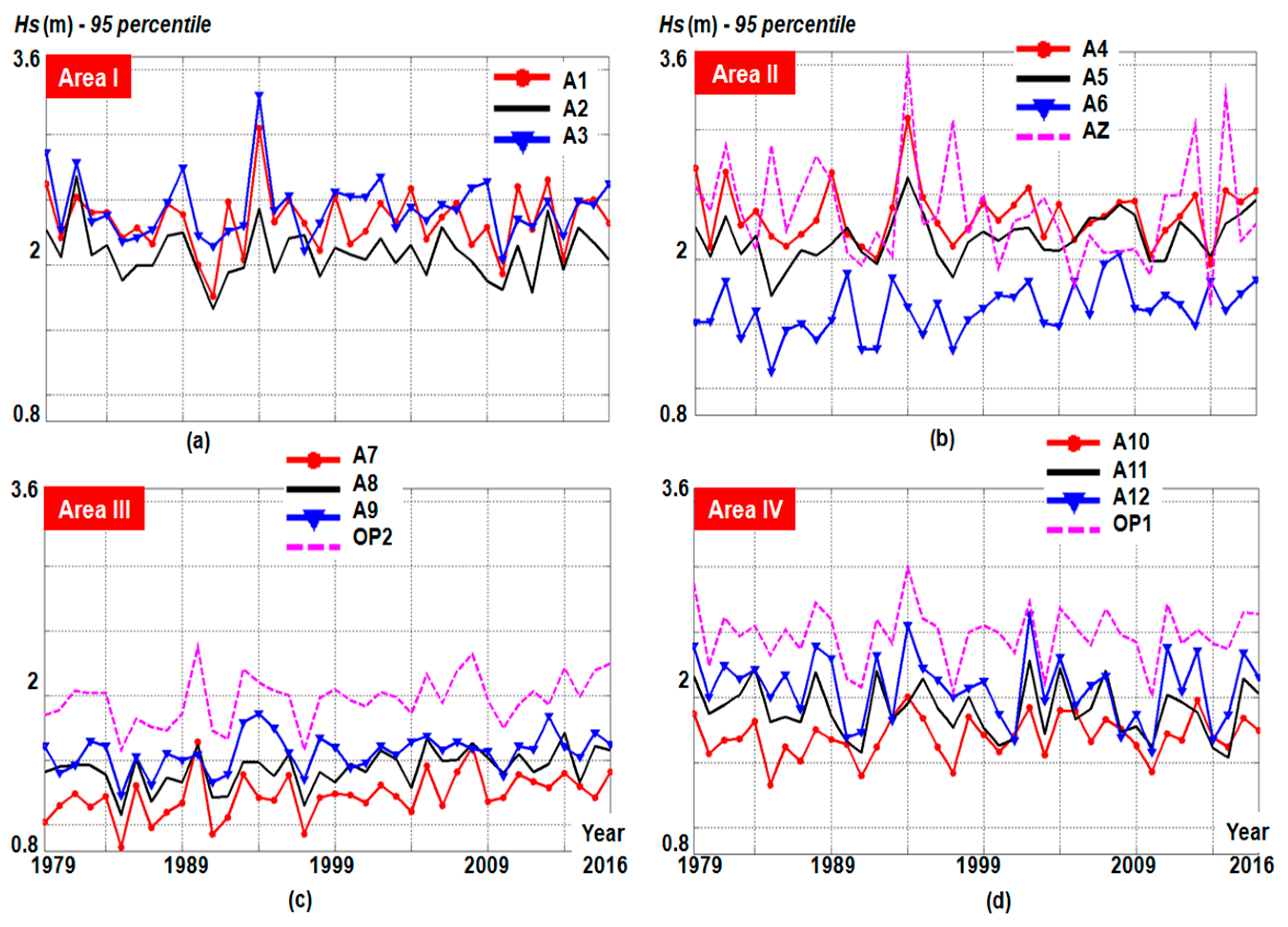
Figure 6.
Hs differences (in meters) between the monthly maximum and minimum average values, corresponding to the inter-annual level. The results cover the 38-year period (1979–2016) of ECMWF wave data, being reported for: (a) Area I; (b) Area II; (c) Area III; (d) Area IV.
Figure 6.
Hs differences (in meters) between the monthly maximum and minimum average values, corresponding to the inter-annual level. The results cover the 38-year period (1979–2016) of ECMWF wave data, being reported for: (a) Area I; (b) Area II; (c) Area III; (d) Area IV.
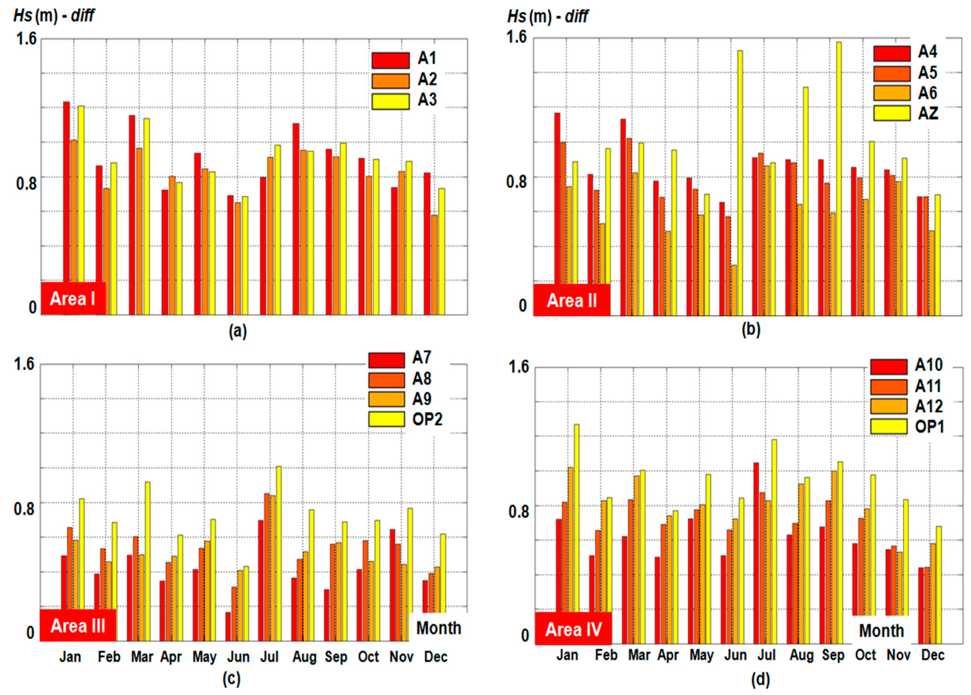
Figure 7.
Monthly sea states related to the values of the Hs parameter based on the 38-year time interval (1979–2016) of ECMWF wave data. The values presented in the diagrams are associated with the moderate conditions, being related to the locations: (a) A1; (b) AZ; (c) A8; (d) OP1.
Figure 7.
Monthly sea states related to the values of the Hs parameter based on the 38-year time interval (1979–2016) of ECMWF wave data. The values presented in the diagrams are associated with the moderate conditions, being related to the locations: (a) A1; (b) AZ; (c) A8; (d) OP1.

Figure 8.
Inter-annual variations of the Hs mean values that resulted from processing the AVISO measurements corresponding to the time interval 2010–2016.The results correspond to the total time (TT) and winter time (WT), respectively, being computed for the points located in: (a) Area I; (b) Area II; (c) Area III; (d) Area IV.

Figure 9.
Inter-annual variations of the maximum Hs values, available for the seven-year time interval (2010–2016) of AVISO satellite measurements. (a) Area I; (b) Area II; (c) Area III; (d) Area IV.
Figure 9.
Inter-annual variations of the maximum Hs values, available for the seven-year time interval (2010–2016) of AVISO satellite measurements. (a) Area I; (b) Area II; (c) Area III; (d) Area IV.
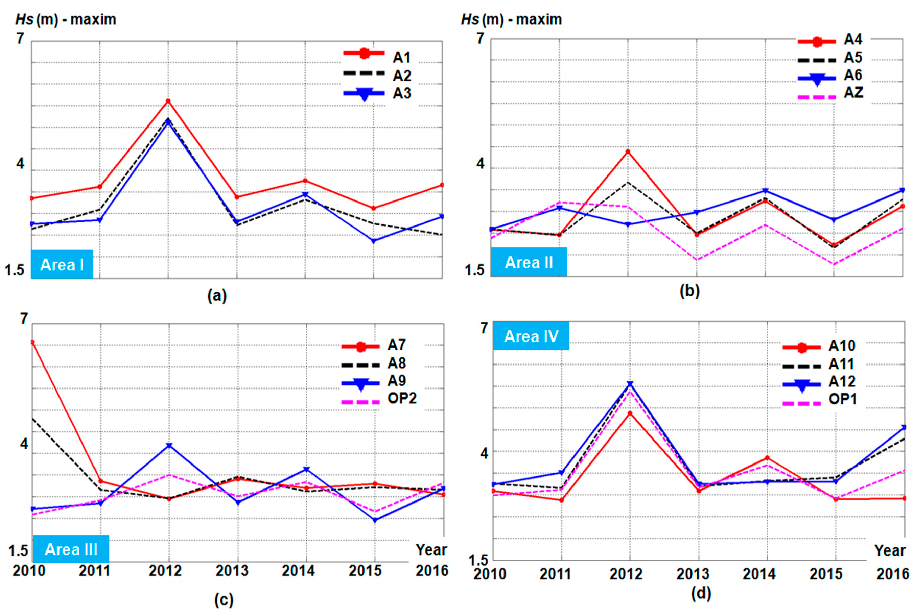
Figure 10.
Monthly variations of the sea states according to the seven-year time interval (2010–2016) of AVISO satellite measurements. Results related to the reference points located in: (a1–a3) → Area I; (b1–b4) → Area II; (c1–c4) → Area III; (d1–d4) → Area IV.
Figure 10.
Monthly variations of the sea states according to the seven-year time interval (2010–2016) of AVISO satellite measurements. Results related to the reference points located in: (a1–a3) → Area I; (b1–b4) → Area II; (c1–c4) → Area III; (d1–d4) → Area IV.
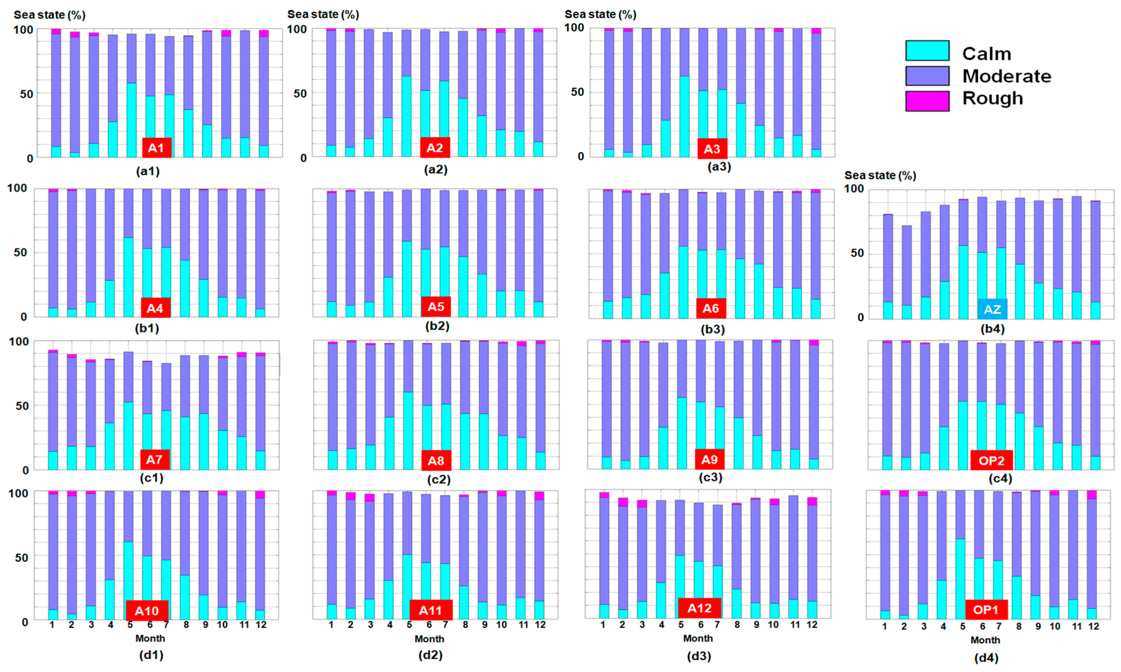
Figure 11.
ECMWF (total time data)—distribution of the significant wave heights for the 38-year time interval (1979–2016), indicated for: (a) mean values; (b) 95 percentile; (c) calm conditions; (d) rough conditions.
Figure 11.
ECMWF (total time data)—distribution of the significant wave heights for the 38-year time interval (1979–2016), indicated for: (a) mean values; (b) 95 percentile; (c) calm conditions; (d) rough conditions.
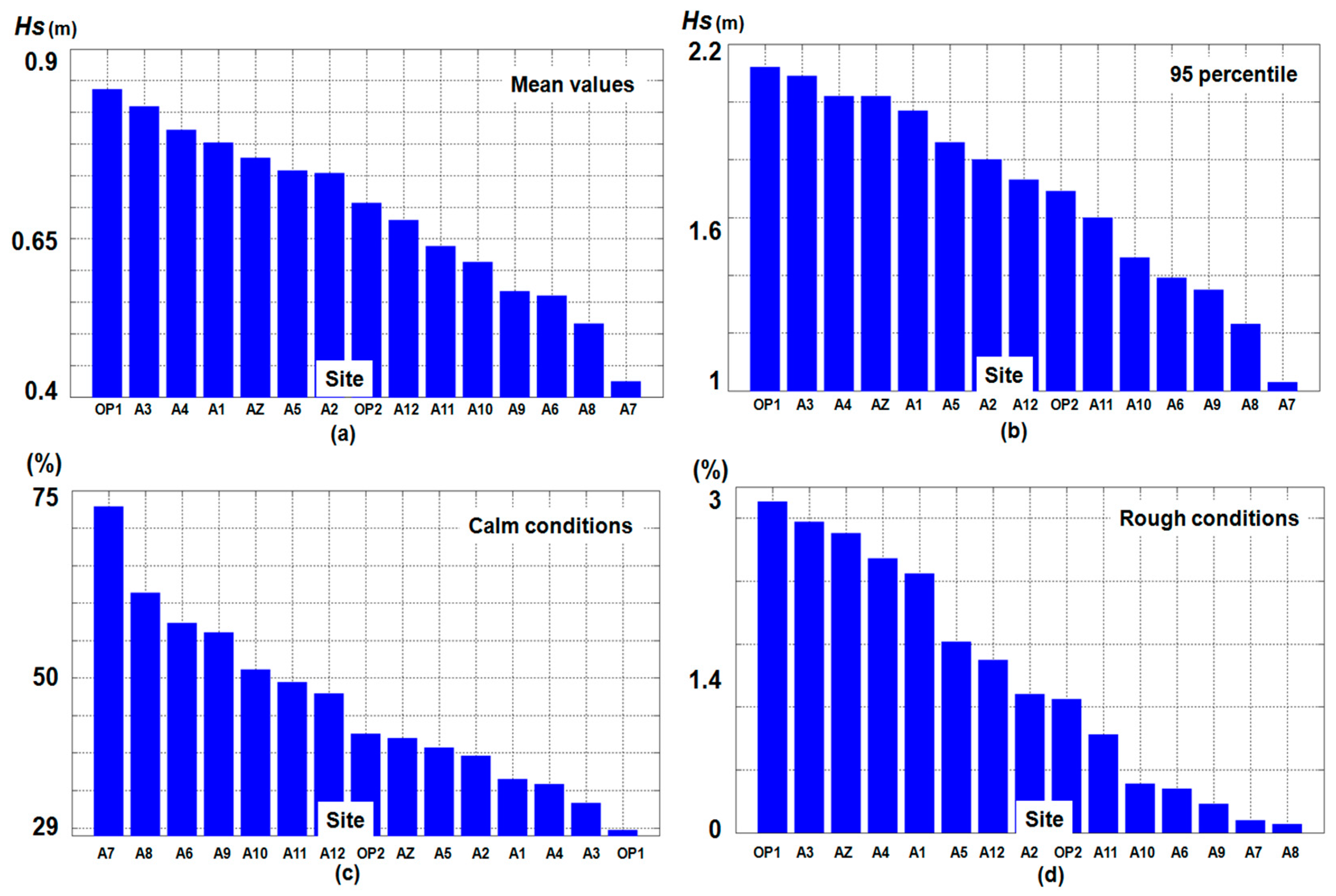
Figure 12.
Temporal and spatial analysis of the AVISO measurements for the seven-year time interval 2010–2016, corresponding to the reference points: (a1–a3) A1 and (b1–b3) A7.
Figure 12.
Temporal and spatial analysis of the AVISO measurements for the seven-year time interval 2010–2016, corresponding to the reference points: (a1–a3) A1 and (b1–b3) A7.

Figure 13.
Estimation of the rough conditions (in %) according to the ECMWF and AVISO data. The results are corresponding to annual scale for the seven-year time interval 2010–2016, being indicated for: (a1–a3) → Area I; (b1–b4) → Area II; (c1–c4) → Area III; (d1–d4) → Area IV.
Figure 13.
Estimation of the rough conditions (in %) according to the ECMWF and AVISO data. The results are corresponding to annual scale for the seven-year time interval 2010–2016, being indicated for: (a1–a3) → Area I; (b1–b4) → Area II; (c1–c4) → Area III; (d1–d4) → Area IV.

Table 1.
Hs statistics resulting from the in situ measurements (Gloria drilling platform) against ECMWF data for the time interval 2003–2009.
Table 1.
Hs statistics resulting from the in situ measurements (Gloria drilling platform) against ECMWF data for the time interval 2003–2009.
| Period | (m) | (m) | Bias (m) | RMSE (m) | SI | R |
|---|---|---|---|---|---|---|
| Total time (TT) | 0.93 | 0.78 | 0.14 | 0.40 | 0.43 | 0.86 |
| Winter time (WT) | 1.11 | 0.96 | 0.15 | 0.44 | 0.39 | 0.88 |
Table 2.
Sea state distribution based on the analysis of 38 years (1979–2016) of ECMWF wave data. The values (in %) are associated to the following sea states: Calm (denoted with C); Moderate (M); Rough (R).
Table 2.
Sea state distribution based on the analysis of 38 years (1979–2016) of ECMWF wave data. The values (in %) are associated to the following sea states: Calm (denoted with C); Moderate (M); Rough (R).
| Interval | 1979–1990 | 1991–2000 | 2001–2016 | 1979–2016 | |||||||||
|---|---|---|---|---|---|---|---|---|---|---|---|---|---|
| Point | C | M | R | C | M | R | C | M | R | C | M | R | |
| A1 | 38.98 | 59.20 | 1.82 | 29.64 | 68.13 | 2.23 | 35.17 | 62.70 | 2.13 | 36.48 | 61.46 | 2.06 | |
| A2 | 41.19 | 57.72 | 1.09 | 31.66 | 67.25 | 1.09 | 39.53 | 59.36 | 1.11 | 39.65 | 59.25 | 1.10 | |
| A3 | 36.48 | 61.21 | 2.31 | 27.76 | 69.61 | 2.63 | 30.89 | 66.62 | 2.49 | 33.29 | 64.24 | 2.47 | |
| A4 | 39.61 | 58.34 | 2.05 | 29.9 | 67.85 | 2.25 | 33.09 | 64.68 | 2.23 | 35.88 | 61.94 | 2.18 | |
| A5 | 44.87 | 53.73 | 1.40 | 34.7 | 63.81 | 1.49 | 36.99 | 61.38 | 1.63 | 40.7 | 57.78 | 1.52 | |
| A6 | 63.08 | 36.59 | 0.33 | 48.71 | 51.00 | 0.29 | 52.22 | 47.38 | 0.40 | 57.29 | 42.36 | 0.35 | |
| A7 | 77.83 | 22.08 | 0.09 | 62.13 | 37.74 | 0.13 | 68.09 | 31.83 | 0.08 | 72.86 | 27.04 | 0.10 | |
| A8 | 66.1 | 33.88 | 0.02 | 52.17 | 47.75 | 0.08 | 56.99 | 42.91 | 0.10 | 61.34 | 38.59 | 0.07 | |
| A9 | 61.9 | 37.92 | 0.18 | 47.02 | 52.72 | 0.26 | 51.57 | 48.19 | 0.24 | 56.11 | 43.66 | 0.23 | |
| A10 | 56.31 | 43.33 | 0.36 | 42.71 | 56.86 | 0.43 | 47.17 | 52.44 | 0.39 | 51.13 | 48.48 | 0.39 | |
| A11 | 49.75 | 49.67 | 0.58 | 41.95 | 57.33 | 0.72 | 48.55 | 50.48 | 0.97 | 49.4 | 49.82 | 0.78 | |
| A12 | 49.64 | 49.12 | 1.24 | 40.66 | 57.97 | 1.37 | 46.19 | 52.35 | 1.46 | 47.96 | 50.67 | 1.37 | |
| OP1 | 32.27 | 65.28 | 2.45 | 25.48 | 71.84 | 2.68 | 27.25 | 70.01 | 2.74 | 29.71 | 67.66 | 2.63 | |
| OP2 | 47.71 | 51.38 | 0.91 | 36.33 | 62.81 | 0.86 | 38.09 | 60.62 | 1.29 | 42.58 | 56.36 | 1.06 | |
| AZ | 42.69 | 54.80 | 2.51 | 33.76 | 63.46 | 2.78 | 42.35 | 55.62 | 2.03 | 41.97 | 55.65 | 2.38 | |
Table 3.
Hs statistics that resulted from processing the AVISO measurements for the time interval 2010–2016, taking into account the total and winter time, respectively.
Table 3.
Hs statistics that resulted from processing the AVISO measurements for the time interval 2010–2016, taking into account the total and winter time, respectively.
| Interval | Total Time | Winter Time | |||||||||||
|---|---|---|---|---|---|---|---|---|---|---|---|---|---|
| Point | Mean (m) | 95th (m) | Max (m) | C (%) | M (%) | R (%) | Mean (m) | 95th (m) | Max (m) | C (%) | M (%) | R (%) | |
| A1 | 0.86 | 2.02 | 5.61 | 25.5 | 69.7 | 1.76 | 1.12 | 2.33 | 5.61 | 5.16 | 84.69 | 3.28 | |
| A2 | 0.78 | 1.72 | 5.21 | 30.15 | 67.89 | 0.94 | 0.99 | 2.04 | 5.21 | 6.80 | 84.53 | 1.72 | |
| A3 | 0.85 | 1.85 | 5.11 | 26.52 | 72.35 | 1.06 | 1.07 | 2.05 | 5.11 | 4.73 | 88.67 | 1.95 | |
| A4 | 0.82 | 1.75 | 4.39 | 27.73 | 71.61 | 0.59 | 1.03 | 1.97 | 4.39 | 5.08 | 88.75 | 1.09 | |
| A5 | 0.78 | 1.73 | 3.68 | 30.31 | 68.17 | 0.39 | 0.99 | 1.94 | 3.68 | 7.12 | 83.91 | 0.78 | |
| A6 | 0.77 | 1.77 | 3.49 | 32.97 | 64.76 | 0.66 | 0.97 | 2.03 | 3.49 | 9.19 | 78.98 | 1.25 | |
| A7 | 0.68 | 1.81 | 6.57 | 31.95 | 54.99 | 1.17 | 0.95 | 2.13 | 6.57 | 10.09 | 67.11 | 2.19 | |
| A8 | 0.77 | 1.82 | 4.79 | 33.44 | 64.25 | 1.02 | 0.96 | 2.05 | 4.79 | 9.54 | 78.05 | 1.72 | |
| A9 | 0.85 | 1.90 | 4.18 | 26.36 | 72.27 | 0.94 | 1.07 | 2.13 | 4.18 | 5.24 | 87.58 | 1.80 | |
| A10 | 0.90 | 1.99 | 4.88 | 24.60 | 73.8 | 1.64 | 1.13 | 2.28 | 4.88 | 4.49 | 87.97 | 3.12 | |
| A11 | 0.89 | 1.97 | 5.55 | 23.70 | 72.43 | 2.31 | 1.11 | 2.36 | 5.55 | 6.49 | 81.95 | 4.22 | |
| A12 | 0.85 | 2.04 | 5.56 | 22.17 | 67.7 | 2.42 | 1.13 | 2.44 | 5.56 | 5.83 | 77.97 | 4.45 | |
| OP1 | 0.90 | 1.99 | 5.38 | 24.29 | 73.41 | 1.95 | 1.14 | 2.29 | 5.38 | 4.58 | 87.03 | 3.67 | |
| OP2 | 0.81 | 1.82 | 3.51 | 29.21 | 68.91 | 0.82 | 1.02 | 2.07 | 3.51 | 6.96 | 83.91 | 1.48 | |
| AZ | 0.76 | 1.50 | 3.22 | 30.15 | 58.66 | 0.16 | 0.86 | 1.66 | 3.11 | 8.25 | 69.38 | 0.23 | |
© 2017 by the authors. Licensee MDPI, Basel, Switzerland. This article is an open access article distributed under the terms and conditions of the Creative Commons Attribution (CC BY) license (http://creativecommons.org/licenses/by/4.0/).
Share and Cite
MDPI and ACS Style
Onea, F.; Rusu, L. A Long-Term Assessment of the Black Sea Wave Climate. Sustainability 2017, 9, 1875. https://doi.org/10.3390/su9101875
AMA Style
Onea F, Rusu L. A Long-Term Assessment of the Black Sea Wave Climate. Sustainability. 2017; 9(10):1875. https://doi.org/10.3390/su9101875
Chicago/Turabian StyleOnea, Florin, and Liliana Rusu. 2017. "A Long-Term Assessment of the Black Sea Wave Climate" Sustainability 9, no. 10: 1875. https://doi.org/10.3390/su9101875
Note that from the first issue of 2016, this journal uses article numbers instead of page numbers. See further details here.