Do Sustainable Stocks Offer Diversification Benefits for Conventional Portfolios? An Empirical Analysis of Risk Spillovers and Dynamic Correlations

Abstract

This paper explores the potential diversification benefits of socially responsible investments for conventional stock portfolios by examining the risk spillovers and dynamic correlations between conventional and sustainability stock indexes from a number of regions. We observe significant unidirectional volatility transmissions from conventional to sustainable equities, suggesting that the criteria applied for socially responsible investments do not necessarily shield these securities from common market shocks. While significant dynamic correlations are observed between sustainable and conventional stocks, particularly in Europe, the analysis of both in- and out-of-sample dynamic portfolios suggests that supplementing conventional stock portfolios with sustainable counterparts improves the risk/return profile of stock portfolios in all regions. The findings overall suggest that sustainable investments can indeed provide diversification gains for conventional stock portfolios globally.

1. Introduction

In the wake of the recent global financial crisis, enormous negative impacts have been felt by conventional institutions and markets. Understandably, a need has been felt for exploring alternatives to conventional financial practices in order to reduce investment risks, increase returns, enhance financial stability, and reassure investors and financial markets. In this regard, academic research on socially responsible investing (SRI), though originally initiated by religious groups like Quakers and Methodists around the eighteenth century [1], has intensified, as has received attention in popular media (http://www.ussif.org/). One reason for the increased interest in SRI investments is that they combine the pursuit of financial returns with non-financial considerations relating to the environment, social issues, and governance (ESG), and hence, are perceived to be less risky compared to conventional alternatives.

As will be seen from the literature review segment below, research on SRI has primarily focused on the risk–return characteristics of these securities in relation to conventional investments. A missing area of research in this regard is whether these securities offer diversification opportunities for conventional investments, based on a formal portfolio allocation exercise. Against this backdrop, our study is the first to address the issue of diversification (or risk hedging) between SRI and conventional investments by considering the regime-switching and volatility interactions between these two types of assets for the entire world economy and a number of regions including North America, Europe and Asia-Pacific. It must be noted that North America and Europe are the largest regions in terms of SRI assets, accounting for 99 percent of the global share for sustainable investing assets [2]. To that end, by examining the risk spillovers and dynamic correlations across SRI investments and conventional assets from different regions, this study provides a comparative analysis of the interaction of these assets with conventional markets, thus enlarging our understanding of whether or not socially responsible investing can indeed benefit investors financially.

In addition to the analysis of dynamic interactions across conventional and SRI assets, we also derive dynamic hedging strategies by adopting a Markov regime-switching Generalized Autoregressive Conditional Heteroskedasticity GARCH model with dynamic conditional correlations (MS-DCC-GARCH). This model allows us to capture both the time-variation in conditional volatility of the markets under consideration according to different regimes and their dynamic links (correlations). By utilizing a time-varying regime-switching specification, we not only account for the well-established nonlinearity that exists in financial markets, but also examine the possibility that SRI significantly reduces the downside risk [3]. Our spillover tests yield significant unidirectional volatility transmissions from conventional to sustainable equities, suggesting that the criteria applied for socially responsible investments do not necessarily shield these securities from common market shocks. While the results from the MS-DCC-GARCH model indicates significant time variation in the dynamic correlations between conventional and sustainable equities, particularly in Europe, the analysis of both in- and out-of-sample portfolios suggests that supplementing conventional stock portfolios with sustainable counterparts improves the risk/return profile of stock portfolios in all regions. Improvement in risk adjusted returns is particularly striking for the broader world index and the Asia-Pacific region when the negative risk adjusted returns for undiversified, conventional portfolios turn around to positive values when the conventional index is supplemented by the sustainable counterpart. However, our portfolio analysis also suggests that these diversification gains can only be achieved by implementing an investment strategy that aims to minimize portfolio risk and utilize sustainable assets in the short leg of the portfolio. The findings overall provide useful guidance for the implementation of effective SRI risk management and for policy regulations. A significant finding of this study is that socially responsible investment does not result in lower risk-adjusted portfolio returns when information on market regimes and dynamic investing strategies are used. This finding is important since it implies that individual investors and fund managers can pursue socially responsible investments without sacrificing returns.

The remainder of the study is organized as follows: Section 2 summarizes the relevant literature and Section 3 presents the MS-DCC-GARCH model used in the analysis. Section 4 describes the data and presents the estimation results, volatility spillover tests and dynamic correlation analysis. Section 5 provides the in- and out-of-sample portfolio performance comparisons and Section 6 concludes the paper.

2. Literature Review

In his pioneering works [4,5], Markowitz lay the foundation for the efficient diversification of investment portfolios and how spreading out a portfolio’s holdings across various assets can improve the risk/return profile for investors. In applications of this concept to socially responsible investments, a number of studies including [1,3,6,7,8,9] claim that non-financial elements provide SRI investors with extra utility or satisfaction. In addition, as pointed out by [1,9,10,11,12], SRI investors tend to believe that ESG factors materially affect the returns in a positive way, which, in turn, can lead to lower costs involved in the avoidance or minimization of environmental and reputational risks, and better management and better customer satisfaction that eventually impacts revenues in a positive way. Possibly, these are the reasons that have led the global SRI (sustainable investment) market to grow steadily both in absolute and relative terms. According to the Global Sustainable Investment Review of 2014 [2], released by the Global Sustainable Investment Association (GSIA), SRI has risen from $13.3 trillion at the outset of 2012 to $21.4 trillion at the start of 2014, which corresponds to an increase from 21.5 percent to 30.2 percent of the professionally managed assets in Europe, the United States, Canada, Asia, Japan, Australasia and Africa.

With support for SRI expanding since the 1960s due to the rise of the civil rights movement, environmentalism and concerns about globalization [1], formal research in this area is not new, and can be associated first with [13]. There are now a number of studies on SRI which have investigated the following aspects, primarily through the lens of mutual funds, but also through regional SRI indexes for not only the US, but also Europe and other major developed economies. (a) Performance (i.e., risk–return characteristics relative to conventional indexes), using mutual funds and broad market indexes [11,12,14,15,16,17,18,19,20,21,22,23,24,25,26,27,28,29,30,31,32,33,34,35,36,37,38] and at firm-level [3,34,39,40,41,42,43,44,45]. These studies, however, fail to provide clear-cut empirical evidence on whether SRI does yield higher returns after adjusting for risks. Similarly, studies on (b) ratings [46,47,48], and (c) screenings [49] in terms of sustainability, do not seem to provide clear cut evidence in terms of higher returns either. Studies of (d) predictability and determinants of returns and volatility [50,51], highlight the role of various forms of uncertainties related to economic policies; and (e) co-movements of SRI indexes and with conventional indexes across various regions [1,52] have been shown to exist, especially when nonlinearity is taken into account.

As can be seen from the above discussion, research on SRI has primarily focused on the risk–return characteristics of these securities in relation to conventional investments. A missing area of research in this regard is whether these securities offer diversification opportunities for conventional investments, based on a formal portfolio allocation exercise. Some tangential discussion regarding diversification is available in [52], where cointegration analysis is performed for the US between the Dow Jones Sustainability Index and the Dow Jones Industrial Average Index. The authors show that while there is no evidence of linear cointegration due to nonlinearity and regime changes, cointegration can be detected using a quantile-regression based approach. This paper then goes on to suggest that this result implies that there are no long-run diversification opportunities in the US between SRI and conventional investments. However, no formal portfolio allocation exercise is performed by [52], which is what we aim to address in this paper based on a MS-DCC-GARCH model, i.e., a variant of the original DCC-GARCH model of [53], with Markov-switching (as detailed in [54]). Note that these types of models have also been widely used in analyzing hedges and safe-haven properties of various assets (see [55] for a detailed discussion in this regard) and also comparing Islamic and conventional equities (see for example, [56] for further details), with the latter being somewhat related to our analysis, given the importance of Sharia rules imposed on screening the equities included in Islamic indices.

3. Methodology

The dynamic conditional correlation (DCC) model used in the study follows [57,58,59] and more recently [60]. Let $R_t=[R_{s,t},R_{c,t}{]}^{\prime }$ be the (2 × 1) vector of returns where $R_{s,t}$ and $R_{c,t}$ are the return on SRI represented by a sustainability index and the return on conventional investment represented by a conventional market index, respectively. The model is constructed in a bivariate fashion with pairs of SRI and conventional investment returns for the entire world economy and a number of regional indexes representing North America, Europe, and Asia-Pacific. The GARCH specification for the volatility spillover model follows [61] and is specified as

$$\begin{array}{l}{R}_t={\mathsf{\Phi }}_0+{\displaystyle \sum _{i=1}^p{\mathsf{\Phi }}_i{R}_{t-i}}+{\epsilon }_t\\ {\epsilon }_t=D_t{z}_t\end{array}$$

(1)

where $D_t=\mathrm{diag}(h_{s,t}^{1/2},h_{c,t}^{1/2})$ is the vector of the conditional volatility terms. The conditional mean of the return vector $R_t$ is specified as a vector autoregressive (VAR) process of order p with (2 × 2) parameter matrices ${\mathsf{\Phi }}_i$, $i=1,2,...,p$. The unexplained component ${\epsilon }_t$ follows a GARCH specification described as ${\epsilon }_t|{\psi }_{t-1}~ID(0,P_t)$ where $P_t$ is the time-varying variance–covariance matrix. Denoting the conditional variance matrix as $H_t=[h_{s,t},h_{c,t}{]}^{\prime }$, we impose the following specification which allows for volatility spillover in the model

$$H_t=c+A{\epsilon }_{t-1}^{(2)}+B{H}_{t-1}$$

(2)

where $c$ is a (2 × 1) vector of constants, $A$ and $B$ are (2 × 2) matrices for the ARCH and GARCH effects and ${\epsilon }_t^{(2)}=[{\epsilon }_{s,t}^2,{\epsilon }_{c,t}^2{]}^{\prime }$. Note that the non-diagonal forms of the matrices $A$ and $B$ allow volatility spillovers across the series. Following [52], we allow conditional correlations to vary over time by specifying the variance–covariance matrix as $P_t=D_t{\Gamma }_t{D}_t$ where ${\Gamma }_t$ is the conditional correlation matrix.

A distinct feature of the model is that the conditional correlation matrix, ${\Gamma }_t$, is characterized by regime-switching as governed by a discrete Markov process and is defined as ${\Gamma }_t=\mathrm{diag}{\left\{Q_t\right\}}^{-1/2}{Q}_t\mathrm{diag}{\left\{Q_t\right\}}^{-1/2}$. In order to incorporate regime shifts into the DCC model shown in Equations (1) and (2), we follow [57] and introduce a Markov regime-switching dynamic correlation model by specifying $Q_t$ as

$$Q_t=[1-\alpha (s_t)-\beta (s_t)]\overline{Q}+\alpha (s_t){\epsilon }_{t-1}^{(2)}+\beta (s_t)Q_{t-1}$$

(3)

where $\overline{Q}$ is the unconditional covariance matrix of the standardized residuals. In Equation (3), $\alpha (s_t)$ and $\beta (s_t)$ are the regime-dependent parameters that control the regime-switching system dynamics where $s_t\in \{1,2\}$ is the state or regime variable following a first-order, two-state discrete Markov process. Note that the variances in this specification are regime-independent whereas the covariances (or correlations) are both time-varying and regime-switching (We estimate the MS-DCC-GARCH model using the two-step approach of [53,62]. In the second step, we use the modified Hamilton filter proposed by [57] to solve the path-dependence problem [63,64,65] and estimate the regime-switching conditional covariances accordingly). As [57] note, the specification in which all parameters are regime dependent is highly unstable due to the large number of switching parameters. Therefore, we restrict the regime dependent structure to the time-varying correlations only. Thus, the model allows both volatility spillovers and regime-switching dynamic correlations. The specification is then completed by defining the transition probabilities of the Markov process as $p_{ij}=P(s_{t+1}=i|s_t=j)$ where $p_{ij}$ is the probability of being in regime i at time t + 1 given that the market was in regime j at time t with regimes i and j taking values in {1, 2}. Finally, the transition probabilities satisfy ${\displaystyle {\sum }_{i=1}^2{p}_{ij}}=1$.

The MS-DCC-GARCH model we specified above has several advantages over the standard DCC-GARCH model. Caporin and McAleer [66] lists and explains ten limitations of the standard DCC-GARCH model. Most of these are technical and the extent of their significance are not well known. How important the technical issues are, usually depends on the complexity of the specification and how far the data is from the assumptions. Two of the limitations, however, might have series consequences for the portfolio analysis. First, as pointed out by [66], the dynamic conditional correlations of the standard DCC-GARCH model are specified for the standardized residuals and, indeed, the standard DCC-GARCH model does not yield dynamic conditional correlations. Second, the standard DCC-GARCH model is not dynamic empirically, because the effect of news in this model is inherently extremely small. Additionally, the standard DCC-GARCH model is a single regime model and completely ignores the typical regime-switching behavior of the financial markets. The MS-DCC-GARCH model used in this study does not have these three limitations of the standard DCC-GARCH models. The MS-DCC-GARCH model has dynamic conditional time varying correlations, is asymmetric in its treatment of the conditional variance matrix and, therefore, is inherently dynamic.

4. Empirical Findings

4.1. Data

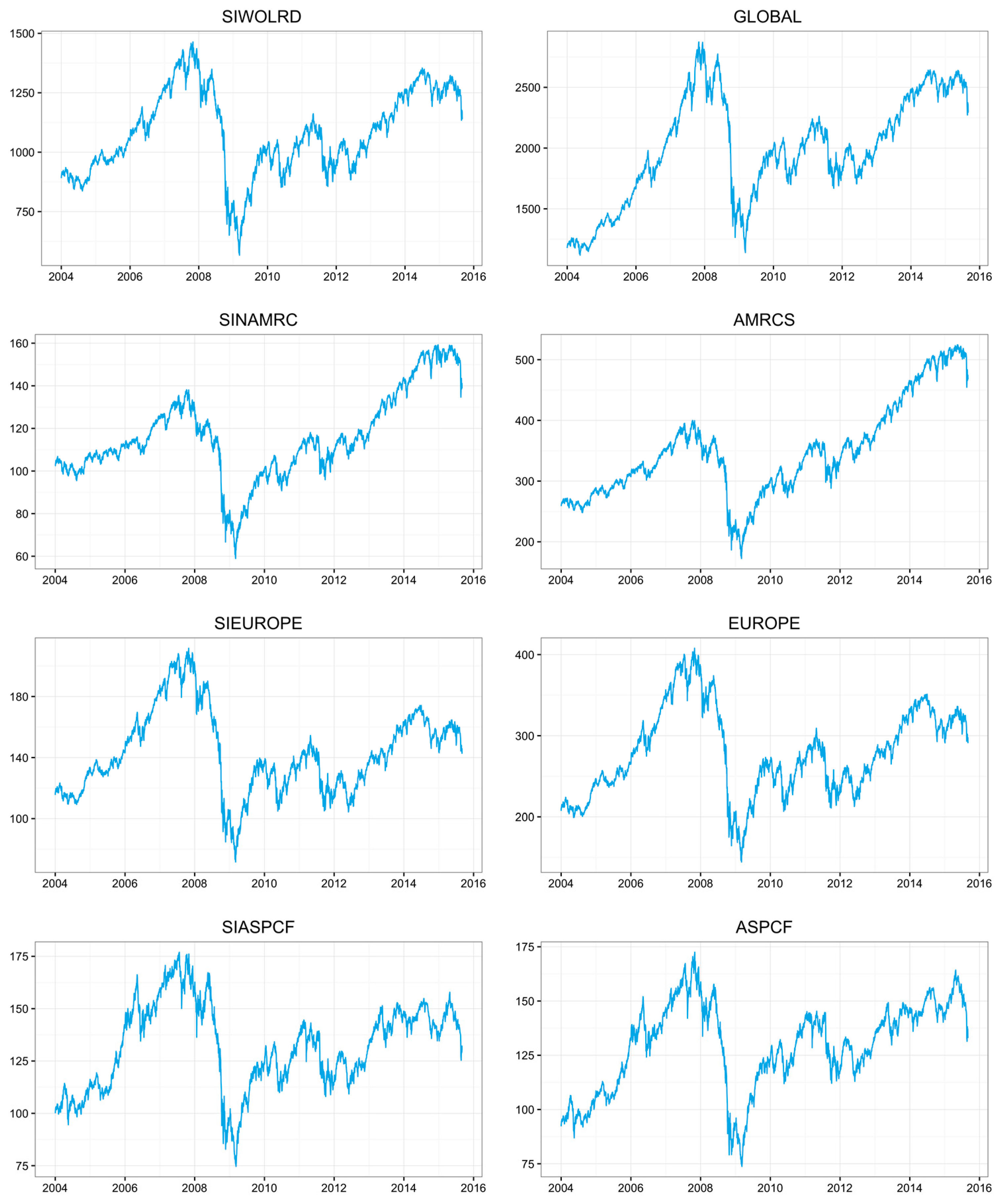
In our empirical analysis, we use daily data for Dow Jones sustainability and conventional indices obtained from Datastream. The conventional indices include the Dow Jones global indices for the World (GLOBAL), North America (AMRCS), Europe (EUROPE) and Asia-Pacific (ASPCF). Similarly, the corresponding Dow Jones sustainability indices for the above-mentioned regions are denoted by SIWORLD, SINAMR, SIEUROPE, and SIASPCF, respectively. The sample period is from 1 January 2004 to 2 September 2015, including 3044 observations.

Table 1. Descriptive statistics for returns (%).

	SIWOLRD	SINAMRC	SIEUROPE	SIASPCF	GLOBAL	AMRCS	EUROPE	ASPCF
Mean	0.01	0.01	0.01	0.01	0.02	0.02	0.01	0.01
S.D.	1.14	1.14	1.45	1.32	1.10	1.22	1.42	1.16
Min	−7.77	−8.99	−9.93	−10.33	−7.89	−9.74	−10.13	−9.11
Max	8.84	9.45	10.46	10.84	9.88	10.51	10.51	9.01
Skewness	−0.30	−0.42	−0.09	−0.34	−0.44	−0.48	−0.12	−0.47
Kurtosis	8.95	11.30	7.59	6.35	9.89	11.40	7.58	6.72
JB	10,227.42 ***	16,313.24 ***	7318.62 ***	5190.91 ***	12,516.18 ***	16,620.02 ***	7301.17 ***	5855.89 ***
Q(1)	34.07 ***	16.53 ***	1.14	0.96	85.75 ***	9.92 ***	0.10	1.32
Q(5)	57.59 ***	31.22 ***	29.83 ***	7.18	98.61 ***	19.57 ***	26.79 ***	4.34
ARCH(1)	120.66 ***	202.02 ***	113.33 ***	94.02 ***	152.65 ***	140.80 ***	100.00 ***	82.70 ***
ARCH(5)	798.47 ***	797.38 ***	593.67 ***	899.63 ***	915.00 ***	789.89 ***	611.35 ***	837.62 ***
n	3044	3044	3044	3044	3044	3044	3044	3044
	Pearson Correlation Coefficient Estimates
	World		Americas		Europe		Asia-Pacific
Full sample	0.966		0.987		0.995		0.976
Subprime Crises Period	0.967		0.992		0.996		0.985

Note: This table gives the descriptive statistics for logarithmic returns. SIWORLD, SINAMR, SIEUROPE, and SIASPCF denote Dow Jones Sustainability Indices (DJSI) for the World, North America, Europe, and Asia-Pacific, respectively, while GLOBAL, AMRCS, EUROPE, and ASPCF denote Dow Jones conventional Global Indices (DJGI) for the World, Americas, Europe and Asia-Pacific. The daily data covers the period 1 January 2004 to 2 September 2015 with n = 3044 observations. In addition to the mean, the standard deviation (S.D.), minimum (min), maximum (max), skewness, and kurtosis statistics, the table reports the Jarque–Bera normality test (JB), the Ljung–Box first (Q(1)), the fourth (Q(5)) autocorrelation tests, and the first (ARCH(1)) and the fourth (ARCH(5)) order Lagrange multiplier (LM) tests for the autoregressive conditional heteroscedasticity (ARCH), and Pearson correlations coefficient estimates. Full sample and subprime mortgage crises period (December 2007–June 2009) Pearson correlation coefficients are reported for World, Americas, Europe, and ASIA-Pacific, which represented the sustainability and conventional index pairs, (SIWORLD GLOBAL), (SINAMRC AMRCS), (SIEUROPE UROPE), and (SIASPCF ASPCF), respectively. The asterisks ***, ** and * represent significance at the 1%, 5%, and 10% levels, respectively.

presents the descriptive statistics for logarithmic returns.

Despite similar values for mean returns, we generally observe higher return volatility for the sustainability indices compared to their conventional counterparts. It can be argued that the economic, environmental and social criteria applied in the selection of firms to be included in these indices limit the potential to mitigate idiosyncratic risks in these portfolios, thus leading to higher return volatility compared to broader based conventional indices. On the other hand, all return series exhibit negative skewness, implying greater likelihood of experiencing losses. Similarly, all return series have kurtosis values higher than the normal distribution, implying the presence of extreme movements. It is possible that the inclusion of the global financial crisis (GFC) in the sample period drives the patterns observed in higher order moments. The impact of the GFC is evident in the time series plots presented in Figure 1. Both conventional and sustainable stock indices sustained significant losses during the 2007/2008 crisis period and then again during early 2012 at the height of the Eurozone crisis.

Table 1 also reports the Pearson correlation coefficient estimates for the pairs of sustainability and conventional indices for each of the four regions, i.e., World, North America, Europe, and Asia-Pacific. The correlations coefficients are reported both for the full sample and the subprime mortgage crises period (December 2007–June 2009) for comparison purposes. Estimates of the correlation coefficients for all regions, both in the full sample and subprime mortgage crises period, are found to be above 96%, suggesting a high degree of co-movement across sustainable and conventional investment returns. While we observe the highest correlation estimates in the case of Europe, we see that correlations do not exhibit a significantly different pattern during the subprime mortgage crises period.

4.2. Model Identification

The MS-DCC-GARCH model requires prior identification of the VAR order p in Equation (1) and univariate GARCH models that are used to obtain conditional volatility estimates in Equations (2) and (3). We first identified the univariate GARCH models using the Akaike information criterion (AIC) to fit the GARCH(1,1) models with a conditional mean that is specified as an autoregressive process of order p, AR(p), leading to a AR(p)-GARCH(1,1) model. We selected the AR order p using the AIC. In order check for possible misspecifications, we performed conditional heteroskedasticity and serial correlation diagnostics. The Lagrange multiplier (LM) test was used for conditional heteroskedasticity diagnosis, while the Ljung–Box portmanteau test (Q) was used for the serial correlation diagnostic.

Table 2. Univariate AR(p)-GARCH(1,1) fit diagnostics.

	ARCH-LM(1)	JB	Q(10)	Q(20)	p
SIWOLRD	2.724	197.383 ***	5.454	19.214	4
	(0.010)	(<0.001)	(0.793)	(0.443)
SINAMRC	5.277 **	427.863***	6.409	17.684	2
	(0.022)	(<0.001)	(0.698)	(0.544)
SIEUROPE	0.122	230.330 ***	4.802	16.135	0
	(0.727)	(<0.001)	(0.851)	(0.648)
SIASPCF	0.001	92.166 ***	4.638	11.789	4
	(0.980)	(<0.001)	(0.865)	(0.895)
GLOBAL	2.160	244.572 ***	4.439	19.661	4
	(0.142)	(<0.001)	(0.880)	(0.415)
AMRCS	5.790	436.193 ***	7.645	18.204	2
	(0.016)	(<0.001)	(0.570)	(0.509)
EUROPE	0.294	220.475 ***	4.543	16.985	0
	(0.588)	(<0.001)	(0.872)	(0.591)
ASPCF	0.311	160.252 ***	7.192	16.732	4
	(0.577)	(<0.001)	(0.617)	(0.608)

Note: The table reports diagnostic tests for univariate autoregressive GARCH model fits. An AR(p)-GARCH(1,1) model was fitted to each series. The AR order p was selected by the Akaike information criterion (AIC). Table reports the Jarque–Bera normality test (JB), the Ljung-Box 10th (Q(10)) and the 20th (Q(20)) autocorrelation tests, and the first (ARCH(1)) order Lagrange multiplier (LM) tests for the autoregressive conditional heteroscedasticity (ARCH). The p-values of the tests are given in parentheses. The asterisks ***, ** and * represent significance at the 1%, 5%, and 10% levels, respectively. The symbol “>” signifies “less than” the number it precedes.

reports the diagnostics for the univariate AR(p)-GARCH(1,1) model and also presents the selected AR orders p where the maximum p was set equal to 10. The selected AR orders vary from 0 to 5 and Ljung–Box tests with the orders 10 and 20 show that the selected orders were sufficient to capture serial correlations in the series. The LM tests do not reject the null of no first order ARCH effects even at the 10% level, except SINAMRC, for which non-rejection occurred only at the 1% level. Given the results in Table 2, we decided that a GARCH(1,1) specification with the AR orders selected by the AIC sufficiently models the conditional heteroskedasticity in all series. In order to select the VAR orders in Equation (1), we used the Bayesian information criterion (BIC) with a maximum order equal to 10. The BIC selected an order of one for all four VAR specifications for the four regions. Finally, the MS-DCC-GARCH models were estimated using the maximum likelihood (ML) method based on these specifications.

4.3. Volatility Spillover Tests

Table 3. Estimates of the MS-DCC-GARCH model.

Parameters	Models
	World	Americas	Europe	Asia-Pasiific
Panel A: Spillover parameters
$c_s$	0.0033 (0.0139)	0.0159 (0.0099)	0.0052 (0.0371)	0.0319 (0.0289)
$c_c$	0.0159 (0.0305)	0.0176 (0.0378)	0.0202 (0.0672)	0.0168 (0.0317)
$a_{s,s}$	0.0358 (0.0304)	0.0162 (0.0303)	0.0189 (0.0821)	0.0173 (0.0562)
$a_{s,c}$	0.0633 (0.7564)	0.0249 (1.9827)	0.0082 (2.8751)	0.0110 (2.8601)
$a_{c,s}$	0.0252 (0.8179)	0.0582 (1.7571)	0.0593 (2.9988)	0.1014 (3.7029)
$a_{c,c}$	0.0337 *** (0.0106)	0.0786 *** (0.0092)	0.0772 ** (0.0365)	0.0945 *** (0.0192)
$b_{s,s}$	0.1266 *** (0.0265)	0.1496 *** (0.0388)	0.2183 *** (0.0590)	0.1549 *** (0.0229)
$b_{s,c}$	0.4627 *** (0.0253)	0.6228 *** (0.0306)	0.4593 *** (0.0721)	0.3965 *** (0.0526)
$b_{c,s}$	0.8503 (0.6626)	0.6612 (2.3041)	0.7239 (2.9214)	0.9425 (2.1682)
$b_{c,c}$	0.4003 (0.7189)	0.3353 (2.0511)	0.4324 (3.0450)	0.3686 (2.8084)
Panel B: DCC parameters
$\alpha \left(s_t=1\right)$	0.0181 *** (0.0036)	0.0427 *** (0.0040)	0.0880 *** (0.0054)	0.0361 *** (0.0060)
$\beta \left(s_t=1\right)$	0.9750 *** (0.0063)	0.9430 *** (0.0058)	0.8528 *** (0.0102)	0.9553 *** (0.0147)
$\alpha \left(s_t=2\right)$	0.0677 *** (0.0250)	0.0839 *** (0.0108)	0.1073 *** (0.0301)	0.0778 * (0.0444)
$\beta \left(s_t=2\right)$	0.7769 *** (0.0999)	0.8730 *** (0.0172)	0.8095 *** (0.0602)	0.8314 *** (0.1668)
Panel C: Regime Inference
log L of MS-DCC	−4029.247	−3084.625	−2785.198	−4495.000
log L of DCC	−5103.762	−4034.694	−3898.901	−5275.907
AIC of MS-DCC	2.661	2.041	1.844	2.968
AIC of DCC	3.360	2.658	2.569	3.474
LR linearity Test	2149.030 ***	1900.138 ***	2227.405 ***	1561.813 ***
$p_{11}$	0.982	0.984	0.969	0.979
$p_{22}$	0.935	0.930	0.889	0.930
$n_1$	2387.100	2478.600	2377.700	2352.100
$n_2$	655.900	564.400	665.300	690.900
Prob(Regime 1)	0.781	0.812	0.781	0.770
Prob(Regime 2)	0.219	0.188	0.219	0.230
Duration of Regime 1	55.140	61.670	32.080	47.740
Duration of Regime 2	15.420	14.320	8.980	14.220

Note: This table reports the estimates of the MS-DCC-GARCH model given in Equations (1)–(3). The matrix R for the World, Americas, Europe, and Asia-Pacific models are formed as R = (SIWORLD GLOBAL), R = (SINAMRC AMRCS), R = (SIEUROPE UROPE), and R = (SIASPCF ASPCF), respectively. The GARCH part of the model is specified as a GARCH(1,1). The subscript $s$ denotes the SRI return series while subscript $c$ denotes conventional return series. The models are estimates over the full sample period 1 January 2004–2 September 2015 with n = 3044 observations. The lag order for the Vector Autoregressive VAR part of the model was selected by the AIC and is one for all four models. The MS-DCC-GARCH model was estimated using the maximum likelihood (ML) method. The likelihood ratio (LR) linearity test is reported with p-value of the [67]. Standard errors of the estimates are given in parentheses. log L stands for the log likelihood, $p_{ii}$ for the regime transition probabilities, Prob (Regime i) for the ergodic (limit) probability of regime i, and $n_i$ for the number of observations falling in regime i according to the ergodic probability. ***, ** and * represent significance at the 1%, 5%, and 10% levels, respectively.

presents the parameter estimates for the MS-DCC-GARCH model described in Equations (1)–(3). As explained earlier, the model is structured to allow for possible bidirectional volatility spillovers across the sustainable and conventional market segments for each global and regional index examined. We observe in Panel A generally insignificant shock spillovers across the sustainable and conventional markets, indicated by insignificant a_ij (i ≠ j) estimates for all regional indexes. On the other hand, significant and positive volatility spillovers are observed from conventional to sustainable indices, implied by highly significant b₁₂ estimates consistently for each region. This finding suggests that uncertainty regarding global equity markets spills over to the market for sustainable stocks, driving return volatility in this market segment. Risk transmissions, however, are found to be unidirectional, implied by insignificant spillover effects from sustainable to conventional indexes. It can thus be argued that sustainable stocks do not necessarily exhibit segmentation from their conventional counterparts and are driven by the common fundamental uncertainties affecting equity markets globally. The findings also suggest that the criteria applied in the identification of socially responsible investments do not necessarily shield these stocks from equity market shocks.

Examining the volatility persistence coefficients measured by (a_ii + b_ii), we generally observe moderate to weak volatility persistence, relatively weaker in the case of sustainable indexes. The volatility persistence coefficients for the conventional (sustainable) indices are estimated as 0.433 (0.162), 0.413 (0.165), 0.509 (0.237), and 0.463 (0.172) for the World, Americas, Europe, and Asia-Pacific regions, respectively. Considering positive own volatility shocks observed in the case of sustainable indexes, implied by highly significant b₁₁ estimates, it can be argued that historical information on return and volatility in sustainable equity markets could be utilized in forecasting future volatility despite the evidence of weak volatility persistence in these markets.

Formal tests of causality in volatility between the conventional and sustainable stock markets are presented in

Table 4. Volatility spillover tests.

Test Type	Wald	NT-R	NT-NR	HH
Panel A: Unidirectional volatility spillovers from conventional to sustainable
$H_0:$ GLOBAL $\Rightarrow$ SIWORLD	26.0335 ***	33.5088 ***	9.9801 ***	7.9773 **
$H_0:$ AMRCS $\Rightarrow$ SINMARC	3.9563	1.7234	5.2534	2.3548
$H_0:$ EUROPE $\Rightarrow$ SIEUROPE	6.9236	3.9381	5.1069	9.6125 **
$H_0:$ ASPCF $\Rightarrow$ SIASPCF	7.2269	5.2085	4.9439	7.6233
Panel B: Unidirectional volatility spillovers from sustainable to conventional
$H_0:$ SIWORLD $\Rightarrow$ GLOBAL	5.7180 *	9.9768 ***	13.6846 ***	3.0029
$H_0:$ SINMARC $\Rightarrow$ AMRCS	1.8908	1.1614	5.285	2.1588
$H_0:$ SIEUROPE $\Rightarrow$ EUROPE	4.4583	2.2569	3.0597	0.338
$H_0:$ SIASPCF $\Rightarrow$ ASPCF	4.7144	3.1005	2.1225	0.3585
Panel C: Bi-directional volatility spillovers between sustainable and conventional
$H_0:$ GLOBAL $\iff$ SIWORLD	19.4387 ***	0.2948	32.5822 ***	42.6304 ***
$H_0:$ AMRCS $\iff$ SINMARC	5.847	2.8848	10.5384 **	4.5136
$H_0:$ EUROPE $\iff$ SIEUROPE	11.3819 **	6.195	8.1666 *	9.9505 **
$H_0:$ ASPCF $\iff$ SIASPCF	11.9413 **	8.3090 *	7.0664	7.9818 *

Note: The table reports causality tests for testing the null hypothesis of no one unidirectional volatility spillover from variable X to variable Y, demoted, X $\Rightarrow$ Y as well as the bidirectional volatility spillover, denoted X $\iff$ Y. The Wald tests for testing the no volatility spillover restrictions were imposed on Equation (1). The tests report that the tests are distributed as Chi-square with 2 and 4 degrees of freedom, respectively, for unidirectional and bidirectional tests. The HH test is the [69] LM test of causality on conditional variance. NT-R is the [68] robust test of the causality in conditional variance, while the NT-NR is the non-robust version of the [68] test. HH, NT-R, and NT-NR tests are LM tests and the univariate specification for conditional variances is a GARCH(1,1) model. We compute HH, NT-R, and NT-NR tests to tests only causality in conditional variance from X variable (Japan or US) to Y variable. ***, ** and * represent significance at the 1%, 5%, and 10% levels, respectively.

. Four alternative spillover tests are utilized to test the null hypothesis of no unidirectional volatility spillover from market X to market Y (X $\Rightarrow$ Y) and no bidirectional spillover between markets X and Y (X $\iff$ Y). The first test is a Wald test involving two zero restrictions on the relevant parameters in matrices A and B in Equation (2). The next two tests are the LM-based robust (NT-R) and non-robust (NT-NR) tests of causality in conditional variance proposed by [68]. Finally, the fourth test (HH) is the Hafner-Herwartz [69] LM test of causality on conditional variance.

Examining the unidirectional spillover tests from the conventional to sustainable indices reported in Panel A, we find that all four tests consistently reject no causality in variance in the case of the broader world index, further supporting prior evidence of significant volatility spillovers from conventional to sustainable stocks. Although not as consistently significant as in the conventional-to-sustainable case, some evidence of volatility spillover in the opposite direction is also found for the world index in Panel B, supported particularly by the causality tests of [68]. On the other hand, the formal unidirectional tests for the other regions reported in Panels A and B did not generally yield evidence of risk transmissions in either direction for regional indices. The tests for bidirectional spillover effects reported in Panel C further support prior findings for the world index, indicating bi-directional risk transmissions across the sustainable and conventional stock indices. On the other hand, we observe largely inconsistent test results for regional indices, consistent with the findings in Panels A and B. Overall, the format tests clearly indicate significant risk transmissions from conventional to sustainable stocks in the case of the world index while somewhat weaker evidence of volatility spillover in the opposite direction is also observed.

4.4. Dynamic Correlations

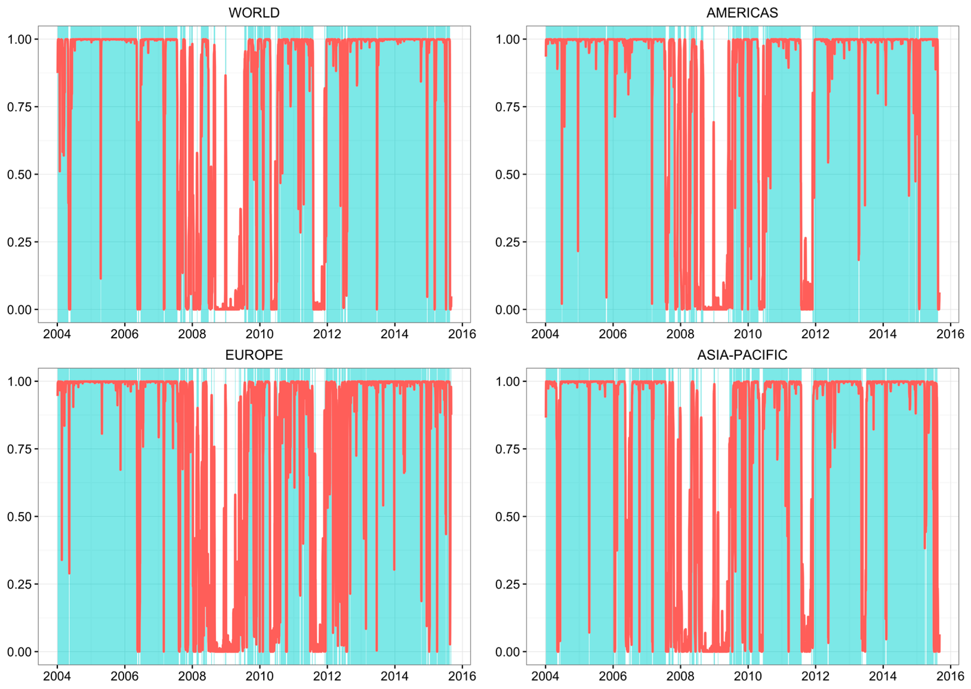
The regime-switching specification that governs the data is tested against the static alternative using a battery of specification tests including the likelihood ratio (LR) linearity test with a p-value of [64], further supported the Akaike (AIC) information criteria. Both formal tests and the information criteria reported in Panel C of Table 3 consistently favor a two-regime MS-DCC-GARCH specification over the static DCC-GARCH alternative, indicating strong support for the presence of two distinct market regimes. The smoothed probability plots for the first regime reported in Figure 2 indicate that the first regime largely corresponds to normal market periods with the smoothed probabilities for this regime dropping to near zero values during the GFC period, as well as the late-2011 and early-2012 periods when the Eurozone uncertainty hit its peak. Therefore, we conclude that the first regime characterizes normal (or low) volatility periods while the second regime is the high volatility regime.

Panel B in Table 3 presents the parameter estimates for the MS-DCC-GARCH model that generates the regime-specific conditional correlations. We observe highly significant $\alpha (s_t)$ and $\beta (s_t)$ estimates in both regime 1 (low volatility) and regime 2 (high volatility), implying significant correlations between the conventional and sustainable market indices in both regimes. The sums $\alpha (s_t)+\beta (s_t)$ are estimated as 0.99 (0.83), 0.98 (0.95), 0.94 (0.90) and 0.99 (0.90) for the low (high) volatility regime for the World, North America, Europe, and Asia-Pacific regions, respectively, suggesting that correlations are highly persistent in both regimes consistently across all regions. Relatively higher values of $\alpha (s_t)+\beta (s_t)$ for the regional indices in both regimes imply that the correlation persistence is more pronounced at the regional level, possibly driven by regional fundamentals driving return dynamics in equity markets.

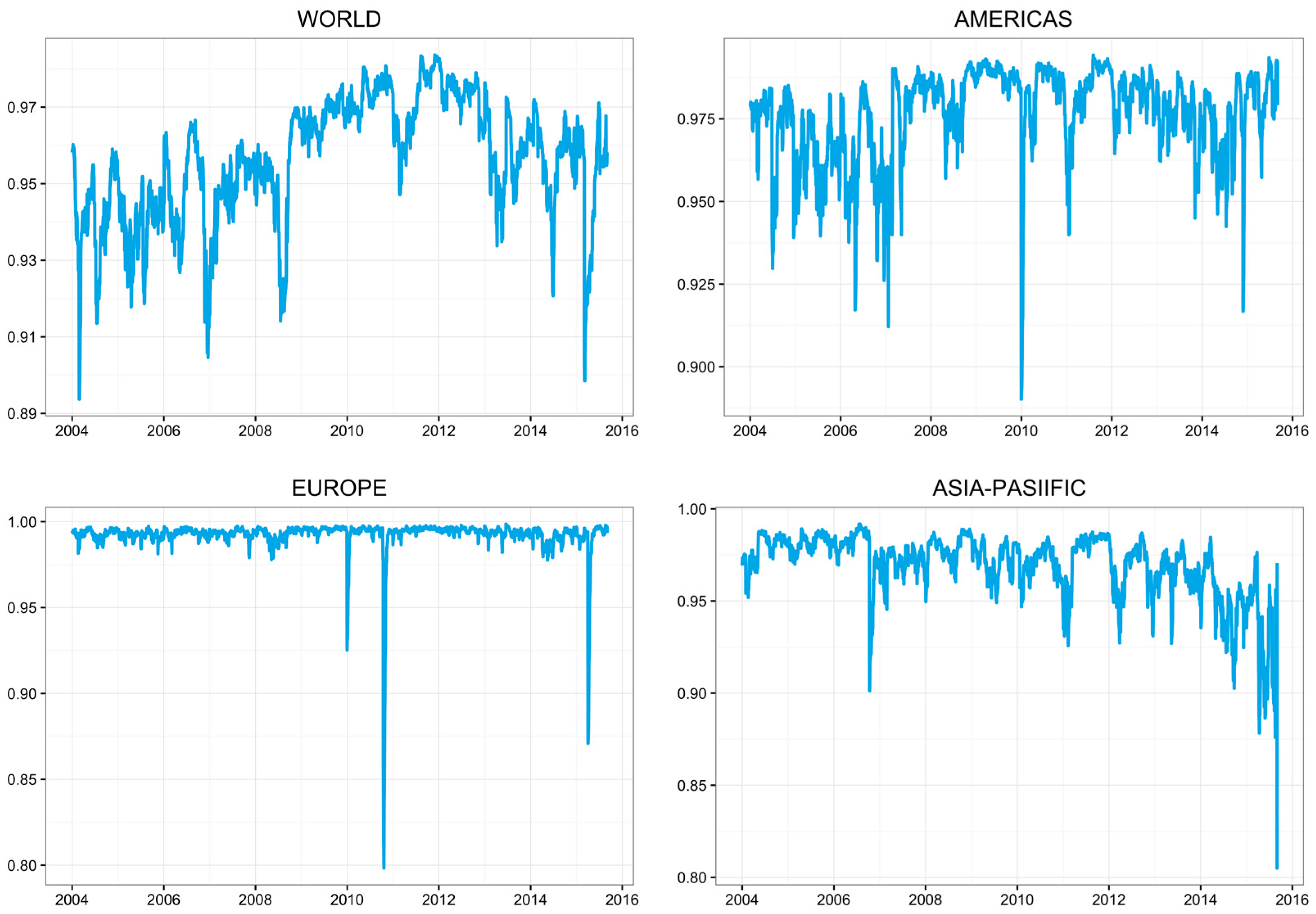
The inferences from the MS-DCC parameter estimates reported in Panel B are further supported by the probability weighted dynamic conditional correlations reported in Figure 3 (The probability weighted time-varying conditional correlations ${\rho }_{ij,t}$ are calculated as ${\rho }_{ij,t}=p_{1,t}{\rho }_{ij,1,t}+\left(1-p_{1,t}\right){\rho }_{ij,2,t}$, where ${\rho }_{ij,\mathrm{k},t}$, $\mathrm{k}=1,2$, are the time-varying conditional correlations in regime $\mathrm{k}$ and $p_{1,t}=P(s_t=1|{\psi }_{t-1})$ is the predictive probability of being in regime 1 at time $t$ given the information set ${\psi }_{t-1}$ available through time $t-1$). The dynamic correlations are highly time-varying for most regions, with the exception of European markets where correlations consistently range in the upper 90%. The significant time variation in the case of the other regional indices, however, further confirms the use of the DCC specification against the constant correlation alternative. Examining the plots in Figure 3, we see that both the global and regional indices exhibit a high degree of association between conventional and sustainable stocks, more consistently in the case of European stocks. Despite the high level of correlations found across all regional indices, however, a somewhat decreasing pattern in conditional correlations is observed for the Asia-Pacific region, suggesting that sustainable securities might have relatively better diversification potential for equity investors in this region. Nevertheless, the dynamic correlations clearly indicate a high degree of association between sustainable and conventional market indices, suggesting that sustainable stocks may have limited diversification benefits for conventional equity portfolios globally.

5. Portfolio Analysis

Having examined the dynamic conditional correlations between sustainable and conventional stocks, we next focus our attention on the risk and return tradeoffs offered by sustainable stocks for conventional equity investors. For this purpose, we consider a currently ‘undiversified’ investor, i.e., an investor who is fully invested in a conventional stock index, and form bivariate portfolios by supplementing the undiversified portfolios with sustainable counterparts one at a time. Two alternative bivariate portfolios are examined, one based on the risk-minimizing portfolio strategy of [70]. (This model follows the dynamic risk-minimizing hedge ratio of [70] computed as ${\theta }_t^{*}=-h_{12,t}/h_{2,t}$ where $h_{i,t}=var\left(R_{i,t}\right)$ and $h_{12,t}=cov\left(R_{1,t},R_{2,t}\right)$ with the subscripts 1 and 2 representing the assets in the bivariate portfolio. In our application, this is based on a $1 long position in the conventional portfolio.) The other is based on the optimal portfolio weight of [71]. (This model follows the minimum-variance portfolio formula of [71], where the regime-independent covariances used in the computation of portfolio weights are obtained as the probability weighted average of regime-dependent covariances with the corresponding predictive regime probabilities as the weights.) A similar procedure is applied in a similar context in [58,59,60,72].

Table 5. Summary statistics for in-sample portfolios.

	Mean	S.D.	Min	Max	HE	Sharpe Ratio
Panel A: World Market
Undiversified Portfolio Return	0.028	1.154	−7.886	9.883	--	0.024
MS-DCC-GARCH Hedged Portfolio Return	0.018	0.295	−1.928	1.961	93.567	0.061
DCC-GARCH Hedged Portfolio Return	0.017	0.293	−1.931	2.026	93.478	0.058
MS-DCC-GARCH Optimal Portfolio Return	0.034	1.012	−8.413	7.775	23.082	0.034
DCC-GARCH Optimal Portfolio Return	0.024	0.940	−6.590	9.883	33.664	0.026
MS-DCC-GARCH Optimal Hedge Ratio	0.929	0.070	0.780	1.209	--	--
DCC-GARCH Optimal Hedge Ratio	0.935	0.059	0.814	1.122	--	--
MS-DCC-GARCH Optimal Portfolio Weight	0.618	0.417	0.000	1.000	--	--
DCC-GARCH Optimal Portfolio Weight	0.635	0.407	0.000	1.000	--	--
Panel B: Americas Market
Undiversified Portfolio Return	0.022	1.268	−9.736	10.515	--	0.017
MS-DCC-GARCH Hedged Portfolio Return	0.010	0.199	−1.177	0.959	97.533	0.050
DCC-GARCH Hedged Portfolio Return	0.009	0.201	−1.177	1.068	97.478	0.045
MS-DCC-GARCH Optimal Portfolio Return	0.009	0.458	−9.453	8.993	16.666	0.020
DCC-GARCH Optimal Portfolio Return	0.009	0.472	−9.453	8.993	14.638	0.019
MS-DCC-GARCH Optimal Hedge Ratio	1.047	0.053	0.828	1.221	--	--
DCC-GARCH Optimal Hedge Ratio	1.042	0.015	0.960	1.080	--	--
MS-DCC-GARCH Optimal Portfolio Weight	0.078	0.216	0.000	1.000	--	--
DCC-GARCH Optimal Portfolio Weight	0.002	0.027	0.000	1.000	--	--
Panel C: European Market
Undiversified Portfolio Return	0.019	1.476	−10.130	10.512	--	0.013
MS-DCC-GARCH Hedged Portfolio Return	0.006	0.149	−1.804	1.601	98.987	0.040
DCC-GARCH Hedged Portfolio Return	0.005	0.149	−1.804	1.601	98.979	0.034
MS-DCC-GARCH Optimal Portfolio Return	0.038	1.429	−10.130	10.512	6.342	0.027
DCC-GARCH Optimal Portfolio Return	0.015	1.466	−10.130	10.512	1.354	0.010
MS-DCC-GARCH Optimal Hedge Ratio	0.977	0.028	0.865	1.088	--	--
DCC-GARCH Optimal Hedge Ratio	0.977	0.006	0.956	0.996	--	--
MS-DCC-GARCH Optimal Portfolio Weight	0.744	0.409	0.000	1.000	--	--
DCC-GARCH Optimal Portfolio Weight	0.980	0.073	0.295	1.000	--	--
Panel D: Asia-Pacific Market
Undiversified Portfolio Return	0.017	1.218	−9.114	9.008	--	0.014
MS-DCC-GARCH Hedged Portfolio Return	0.005	0.239	−1.431	1.434	96.135	0.021
DCC-GARCH Hedged Portfolio Return	0.003	0.240	−1.340	1.295	96.104	0.013
MS-DCC-GARCH Optimal Portfolio Return	0.016	1.094	−9.114	9.008	3.775	0.015
DCC-GARCH Optimal Portfolio Return	0.017	1.192	−9.114	9.008	0.000	0.014
MS-DCC-GARCH Optimal Hedge Ratio	0.854	0.052	0.700	1.052	--	--
DCC-GARCH Optimal Hedge Ratio	0.851	0.005	0.837	0.868	--	--
MS-DCC-GARCH Optimal Portfolio Weight	0.977	0.130	0.000	1.000	--	--
DCC-GARCH Optimal Portfolio Weight	1.000	0.000	1.000	1.000	--	--

Note: The in-sample period covers 2 January 2004–19 February 2014 with 2644 observations. HE stands for the hedge effectiveness index.

presents the summary statistics for the in-sample period covering 2 January 2004–19 February 2014, with 2644 observations. We report in the table the summary statistics for portfolio returns as well as the optimal portfolio weights based on the portfolio strategies of [70,71]. Hedge effectiveness (HE), measured as the percentage of portfolio return volatility that is reduced by supplementing the undiversified portfolio with the sustainable index, along with the corresponding Sharpe ratios, are also reported in the table. Panels A, B, C and D in Table 5 present the findings for the ‘undiversified’ stock portfolios representing an investor who is currently fully invested in the conventional Dow Jones World, Americas, Europe, and Asia-Pacific indices, respectively. In each panel, the row labeled ‘undiversified’ provides the summary statistics for an undiversified investor who is currently fully invested in the corresponding conventional market.

As expected, the risk-minimizing portfolio strategy of [70] yields the largest reduction in return volatility, consistently in all panels. For example, focusing on Panel A, while the undiversified portfolio that is fully invested in the conventional world index has return volatility of 1.154%, supplementing the portfolio with the sustainable counterpart helps reduce portfolio risk down to 0.295% (0.293%), leading to a 93.5% (93.4%) reduction in portfolio volatility based on the MS-DCC (DCC) specification, respectively. Clearly the high conditional correlations between the conventional and sustainable stock indices reported earlier help reduce return volatility in the hedged portfolio as the strategy by [70] takes a short position in the corresponding sustainable index. On the other hand, the optimal portfolio weight strategy of [71] does not work as effectively in mitigating portfolio risk, yielding about 33% risk reduction at best in the case of the world index in Panel A.

Examining the Sharpe ratios reported in the last column in each panel, we observe that supplementing the conventional portfolio with a position in the sustainable counterpart leads to a significant improvement in risk-adjusted returns in all panels. The improvement in Sharpe ratios is especially evident in the case of the risk-minimizing portfolio strategy of [70], where risk-adjusted returns are more than double in most regions, with the exception of Asia-Pacific in Panel D. Furthermore, comparing the risk adjusted returns and hedge effectiveness values for the MS-DCC-GARCH- and DCC-GARCH-based portfolios, we observe that the MS-DCC-GARCH model yields more favorable outcomes across all panels, underscoring the superiority of dynamic specification over the static counterpart. Overall, the in-sample portfolio findings reported in Table 5 suggest that supplementing conventional stock portfolios with their sustainable counterparts could both help reduce portfolio volatility and yield much improved risk-adjusted returns. However, this can only be achieved following the risk-minimizing portfolio strategy of [70], which takes advantage of the high correlations between the conventional and sustainable stocks by taking a short position in the sustainable index.

The in-sample portfolio results reported in Table 5 are further supported by the out-of-sample results reported in

Table 6. Summary statistics for out-of-sample portfolios.

	Mean	S.D.	Min	Max	HE	Sharpe Ratio
Panel A: World Market
Undiversified Portfolio Return	−0.015	0.686	−3.986	2.119	--	-0.022
MS-DCC-GARCH Hedged Portfolio Return	0.008	0.219	−1.154	1.369	89.818	0.037
DCC-GARCH Hedged Portfolio Return	0.008	0.220	−1.206	1.375	89.712	0.036
MS-DCC-GARCH Optimal Portfolio Return	0.018	0.525	−2.284	3.038	41.380	0.034
DCC-GARCH Optimal Portfolio Return	0.010	0.566	−2.284	2.488	32.011	0.018
MS-DCC-GARCH Optimal Hedge Ratio	0.916	0.069	0.760	1.071	--	--
DCC-GARCH Optimal Hedge Ratio	0.927	0.041	0.844	1.025	--	--
MS-DCC-GARCH Optimal Portfolio Weight	0.648	0.390	0.000	1.000	--	--
DCC-GARCH Optimal Portfolio Weight	0.734	0.299	0.000	1.000	--	--
Panel B: Americas Market
Undiversified Portfolio Return	0.002	0.792	−3.988	3.438	--	0.003
MS-DCC-GARCH Hedged Portfolio Return	0.006	0.141	−0.661	0.458	96.830	0.043
DCC-GARCH Hedged Portfolio Return	0.006	0.152	−0.649	0.500	96.287	0.039
MS-DCC-GARCH Optimal Portfolio Return	0.005	0.700	−2.903	3.438	21.883	0.007
DCC-GARCH Optimal Portfolio Return	0.003	0.800	−3.552	3.853	−2.088	0.004
MS-DCC-GARCH Optimal Hedge Ratio	0.995	0.050	0.864	1.161	--	--
DCC-GARCH Optimal Hedge Ratio	1.037	0.011	0.994	1.073	--	--
MS-DCC-GARCH Optimal Portfolio Weight	0.370	0.421	0.000	1.000	--	--
DCC-GARCH Optimal Portfolio Weight	0.001	0.011	0.000	0.153	--	--
Panel C: European Market
Undiversified Portfolio Return	−0.040	0.917	−3.182	3.122	--	−0.044
MS-DCC-GARCH Hedged Portfolio Return	−0.001	0.132	−1.067	1.181	97.930	−0.008
DCC-GARCH Hedged Portfolio Return	−0.002	0.132	−1.095	1.181	97.928	−0.015
MS-DCC-GARCH Optimal Portfolio Return	−0.032	0.827	−2.911	3.122	18.625	−0.039
DCC-GARCH Optimal Portfolio Return	−0.039	0.891	−3.182	3.122	5.500	−0.044
MS-DCC-GARCH Optimal Hedge Ratio	0.975	0.029	0.840	1.060	--	--
DCC-GARCH Optimal Hedge Ratio	0.981	0.006	0.967	0.997	--	--
MS-DCC-GARCH Optimal Portfolio Weight	0.734	0.393	0.000	1.000	--	--
DCC-GARCH Optimal Portfolio Weight	0.933	0.165	0.200	1.000	--	--
Panel D: Asia-Pacific Market
Undiversified Portfolio Return	−0.019	0.708	−4.425	2.146	--	−0.027
MS-DCC-GARCH Hedged Portfolio Return	0.003	0.328	−4.267	0.851	78.579	0.009
DCC-GARCH Hedged Portfolio Return	0.002	0.332	−4.370	0.886	78.034	0.006
MS-DCC-GARCH Optimal Portfolio Return	−0.007	0.639	−2.305	2.146	18.430	−0.011
DCC-GARCH Optimal Portfolio Return	−0.019	0.708	−4.425	2.146	0.000	−0.027
MS-DCC-GARCH Optimal Hedge Ratio	0.824	0.063	0.686	1.080	--	--
DCC-GARCH Optimal Hedge Ratio	0.845	0.005	0.835	0.861	--	--
MS-DCC-GARCH Optimal Portfolio Weight	0.928	0.222	0.000	1.000	--	--
DCC-GARCH Optimal Portfolio Weight	1.000	0.000	1.000	1.000	--	--

Note: The out-of-sample period covers 20 February 2014–2 September 2014 with 400 observations. HE stands for the hedge effectiveness index.

. The out-of-sample period covers 20 February 2014–2 September 2014, including 400 observations, with the estimates obtained as one-step forecasts recursively during the out-of-sample period. Consistent with the findings in Table 5, we observe that the risk-minimizing portfolio strategy yields a significant reduction in portfolio risk when the conventional index is supplemented by a position in the sustainable counterpart. The largest risk reduction is observed for the Americas (Panel B) and Europe (Panel C), with more than 96% of return volatility eliminated in the hedged portfolio. Interestingly, hedging the conventional portfolio risk with a short position in the sustainable counterpart also helps improve the risk/return profile of the portfolio in all regions. More strikingly, the negative Sharpe ratios observed for the World and Asia-Pacific indexes turn around to positive risk adjusted returns when the conventional index is supplemented by the sustainable counterpart. A similar improvement in risk-adjusted returns is also observed in other panels, indicating significant diversification benefits from sustainable stocks. In sum, despite the high conditional correlations observed between conventional and sustainable market indices, the analysis of both in- and out-of-sample portfolios clearly suggest significant diversification gains from supplementing conventional portfolios by positions in sustainable stocks. However, these diversification gains can only be achieved by implementing the risk-minimizing portfolio strategy of [67], which takes advantage of the high correlations by taking opposite positions in the conventional and sustainable portfolios.

6. Conclusions

This paper explores the potential diversification benefits of socially responsible investments for conventional stock portfolios by examining the risk transmissions and dynamic correlations between conventional and sustainable stock indices from a number of regions. Utilizing a Markov regime-switching GARCH model with dynamic conditional correlations (MS-DCC-GARCH), we find evidence of significant and positive volatility spillovers from conventional to sustainable equities, suggesting that uncertainty regarding global equity markets spills over to the market for sustainable stocks, driving return volatility in this market segment. Risk transmissions, however, are found to be unidirectional, implied by largely insignificant spillover effects from sustainable to conventional indexes. We argue that the economic, environmental and social criteria applied in the selection of firms to be included in socially responsible indices do not necessarily shield these stocks from common equity market shocks. Despite the presence of risk transmissions from conventional markets, however, our findings also suggest that historical information on return and volatility in sustainable equity markets could be utilized in forecasting future volatility in these markets. Thus, investors and trustees of institutional funds who are concerned about stability in the market for sustainable investments should not only monitor volatility in global conventional markets, but also supplement their volatility forecasting models by measures of historical risk and return dynamics in these markets.

Similarly, the analysis of dynamic conditional correlations suggests that both the global and regional indices exhibit a high degree of association between conventional and sustainable stocks, more consistently in the case of European stocks. Although significant time-variations in the dynamic correlations are observed between conventional and sustainable stock returns, we estimate particularly high correlations that consistently range in the upper 90% in the case of Europe. Interestingly, however, despite the high correlations observed, the analysis of both in- and out-of-sample portfolios suggests that significant diversification gains can be obtained from supplementing conventional portfolios by positions in sustainable stocks. Improvement in risk adjusted returns is particularly striking for the broader world index and the Asia-Pacific region when the negative Sharpe ratios for undiversified, conventional portfolios turn around to positive values when the conventional index is supplemented by the sustainable counterpart. However, our portfolio analysis also suggests that these diversification gains can only be achieved by implementing an investment strategy that aims to minimize portfolio risk and utilize sustainable assets in the short leg of the portfolio.

Given the availability of various exchange-traded funds that allow investors to choose investments based on social and personal criteria, our findings have significant implications for both retail and institutional investors. Thanks to the rapid growth experienced in the SRI market segment, investors have their choices when it comes to allocating parts of their portfolios in various exchange traded funds that reflect this growing segment. Furthermore, the fact that these funds are offered to investors at low cost makes transaction costs less of a concern from a retail investor perspective. More importantly, unlike the case for individual stocks, for which uptick rules apply, diversifying into SRIs via short positions in exchange traded funds that do not have the uptick rules means that investors will have greater flexibility in the creation of diversified portfolios as we recommend in our empirical results. Overall, the findings suggest that sustainable investments can indeed provide significant diversification gains for conventional stock portfolios globally and the fact that these investments are easily accessible at low cost via a myriad of exchange traded funds makes them an appealing investment tool both for retail and institutional investors.