Characteristic Rain Events: A Methodology for Improving the Amenity Value of Stormwater Control Measures

Abstract

Local management of rainwater using stormwater control measures (SCMs) is gaining increased attention as a sustainable alternative and supplement to traditional sewer systems. Besides offering added utility values, many SCMs also offer a great potential for added amenity values. One way of achieving amenity value is to stage the rainwater and thus bring it to the attention of the public. We present here a methodology for creating a selection of rain events that can help bridge between engineering and landscape architecture when dealing with staging of rainwater. The methodology uses quantitative and statistical methods to select Characteristic Rain Events (CREs) for a range of frequent return periods: weekly, bi-weekly, monthly, bi-monthly, and a single rarer event occurring only every 1–10 years. The methodology for selecting CREs is flexible and can be adjusted to any climatic settings; here we show its use for Danish conditions. We illustrate with a case study how CREs can be used in combination with a simple hydrological model to visualize where, how deep and for how long water is visible in a landscape designed to manage rainwater.

1. Introduction

Sustainable Urban Drainage Systems (SUDS), Water Sensitive Urban Design (WSUD), Low Impact Development (LID), Best Management Practices (BMPs) and Stormwater Control Measures (SMCs) are concepts that have gained increasing attention in recent years [1]. The different terms reflect different visions and scopes as well as drivers and priorities, but they generally refer to a similar set of technologies for managing stormwater. Here, SMCs is used. These technologies generally use local detention, retention, infiltration and evaporation to reduce the amount of stormwater leaving a site. They stand in contrast to traditional stormwater management technologies, i.e., mainly underground infrastructure such as pipes and basins, which generally focus on transporting stormwater away from urban areas as efficiently as possible without causing overflows.

SCMs have a potential to deliver multiple additional benefits besides managing stormwater [2,3,4]. It is often claimed that delivering added benefits with SCMs is crucial for their successful implementation [5,6,7]. A number of projects demonstrate that it is possible to achieve stormwater management goals and in addition enhance the value of the local urban setting [8]. However, there are also examples of less successful projects where the designs do not deliver the expected aesthetic value. A review of 20 European SCM-based projects [9] identified two key parameters in the design that were found crucial to successful stormwater management landscape projects: water dynamics and water accentuation. They concluded that many projects accentuate stormwater features, which in practice are presenting only little water, leading to a disproportion between water and other materials appearing like “dry craters” in the urban landscape. The authors (ibid) [9] in conclusion questioned whether the designers were aware of the dynamics of the amount of water for which they were designing. Backhaus, Dam and Jensen [10] similarly identified dimensioning as one of the major challenges for landscape architects undertaking design of SCMs. Based on observations of the design process and interviews they concluded that simple tools that reflect the distribution of rainfall events would be relevant and valuable for designers. This study aim to develop such a tool, which can help designers improve the amenity value of SCMs through successful staging of water.

1.1. Utility, Amenity and the Staging of Rainwater

Given the multiple benefits that SCMs can deliver, it can be useful to categorize them. Several theoretical frameworks can be used to do so, e.g., the concept of ecosystem services [11,12,13,14]. This concept was one of the inspiration sources for the recently developed “Copenhagen Model” for valuing urban nature in the context of climate adaptation [15]. This model distinguishes between “amenity values” (including belonging, coexistence, learning, sensing and community) and “utility values” (including rainwater management, microclimate regulation, CO₂ reduction, noise reduction, air quality improvement, water quality control, and food cultivation). This distinction is in line with one proposed by Echols and Pennypacker [7,16], who used them in the more narrow context of stormwater management; here the “utility goals… provide for hydrological function that protects public health, safety, welfare and aquatic habitat” [16], while “amenity is understood as a feature focused on the experience of stormwater in a way that increases the landscape’s attractiveness or value” [16].

In this paper, the focus is on how to successfully stage rainwater in SCMs. “Staging rainwater” is formulated as designing a landscape feature that actively displays rainwater when it is present, drawing attention to the water itself and to the functionality that the landscape feature has in managing the rainwater. Staging the water is considered a means of achieving some of the amenity values defined by, e.g., the Copenhagen Model and Echols and Pennypacker. The following two sections contain brief reviews of existing tools that have the objective of supporting designers in achieving amenity values and supporting engineers in achieving utility values, respectively.

1.2. Tools to Support Amenity Design

Planning and design tasks are often characterized by a high level of complexity and uncertainty, as many different factors come into play at each specific site, especially so when the new design is being retrofitted into an existing city. Therefore, such tasks are often referred to as “wicked problems” [17] that cannot be solved by linear processes, but need a creative designer to find a good solution for the given context, while considering the social factors. The design work of landscape architects is a creative process, which differs for each individual. Idea generation in the creative process is still accepted to be a “black box”, even though different authors such as Andersson [18] and Lawson [19] have tried to give explanations. What seems to be common for the creation of a landscape design is the iterative character of the process that includes phases of analysis, synthesis, construction, testing and evaluation, with different kinds of technical, spatial, experimental or social knowledge being considered [20,21].

To aid such a process, methods for area analysis (e.g., [22,23]), inspiration from case descriptions of comparable projects (e.g., [24,25]), or inspiration from art and history or a site’s specific identity, go together with technical guidelines, laws and regulations. Additionally, specific design tools for climate change adaptation purposes, such as software or written manuals (e.g., [26,27]), might support the design process.

Backhaus, Dam, and Jensen [10] claim that, to improve stormwater management for amenity design, technical guidelines such as methods for dimensioning, need to be adapted to the designers’ needs and working methods. Additionally, it seems helpful to clearly state criteria and goals for “good stormwater design”. Echols and Pennypacker [7,16] were some of the first to offer designers advice on how to create what they call “artful rainwater design” (i.e., environmentally responsible stormwater management that also “educates and delights those who visit” [16]). They defined five overall goals for the amenity design: education, recreation, safety, public relations and aesthetic richness. However, none of these general goals, nor the more specific objectives or the design techniques they offer for achieving the goals, explicitly address staging of water.

1.3. Tools to Support Utility Design

Tools used to support engineers when designing stormwater management systems are often referred to as decision support tools. Such tools are often mathematical models of drainage systems where the engineer can set up different designs, simulate performance under different rainfall scenarios, and work towards a solution that optimizes the relevant goals, such as frequency of sewer surcharge, frequency of sewer overflows, etc. Reviews of simulation models used for designing and studying SCM systems can be found in [28,29], while reviews of a wider range of tools supporting choice of SCMs, including utility values such as minimizing greenhouse gas emissions and regulating microclimate, can be found in, e.g., [30].

Regarding rainfall, even through use of historical or synthetically rainfall time series for design is an emerging field [31] the typical engineering approach is still to construct a synthetic rainfall event with the desired return period to match the functional requirements for the drainage system [32]. Such a rainfall event is referred to as a design storm, and it is constructed based on rainfall statistics such that it represents the worst case scenario in accordance with the fail-safe philosophy generally used in infrastructure planning [33]. Design storms have also been used to design SCMs (e.g., [34,35]) with respect to delivering utility values, but, to our knowledge, they have never been applied with respect to delivering amenity values.

1.4. Bridging between Amenity and Utility Designs

The short review of design support tools provided above demonstrates that landscape architects generally have access to “soft” (descriptive) tools while engineers use “hard” (quantitative) tools.

To ensure utility values, engineers design for “worst case” scenarios by use of synthetic rain events representing the worst imaginable case based on statistical properties. These rain events will determine the overall detention–retention volume required of an SCM. Within this requirement, the shape of the SCM can vary, and this is where the landscape architect’s design skills come into play. To envision how water will appear in the SCM on a more frequent basis, it is useful to know more about more frequent rains. It would be possible to use the statistical methods of the engineers and create more frequent synthetic rains, but by picking a few representative historic rain events the output can be much more “tangible” and the design process run smoothly.

To bridge between amenity and utility values the Three Points Approach (3PA) was used. The 3PA is a conceptual model developed to facilitate interdisciplinary communication regarding urban stormwater management solutions [36,37]. The approach identifies three unique domains of rainfall where different rules, stakeholders and priorities dominate. Traditionally, stormwater management has only addressed the utility value, where dimensioning criteria, environmental regulations, etc. prescribe how utility companies must design and operate stormwater management systems. Increasing urbanization, together with expected increase in frequency of larger storms due to climate change, has resulted in an increased interest in reducing cities’ vulnerability to flooding, calling for solutions targeting extreme events. At the same time, increasing demands for sustainability and livability, i.e., amenity values, can be interpreted as an increased interest in small rains with higher frequency (everyday rain).

1.5. Aim and Content

The aim of this study was to develop a methodology for producing a set of Characteristic Rain Events (CREs) for landscape architects to use in the design of SCMs in order to improve amenity values without compromising utility values. It is assumed that a set of specific, historic rain events that represent the more frequent rains in a given climate may provide a better insight into the varying nature of rainfall, and further that such a specific dataset can support testing of designs and thus more easily identify the optimal dimensions of the varies sub-volumes making up the necessary detention–retention volume of the SCM. In the following sections, the methodology developed for choosing CREs is described; the concept is illustrated by presenting the resulting CREs for Greater Copenhagen, Denmark, and by showing how these CREs are used to evaluate an SCM design case study. Finally, the strengths and weaknesses of the methodology are discussed.

2. Methodology

2.1. Analysis of Rainfall Records

2.1.1. Rainfall Data and Aggregation of Rain Events

The CREs were extracted from a 36-year rain record covering the period 1979–2015 obtained from a tipping bucket rain gauge with 1 min recordings located in Copenhagen, Denmark. SCMs generally have a detention volume for delay before discharge, and/or a retention volume from where the water can infiltrate and evaporate. Depending on a combination of natural parameters (such as the soil’s hydraulic conductivity) and design requirements (such as the maximum allowed rate of flow out of the SCM), water will empty from the SCM and the detention–retention volume of the SCM will be regained. Many places, a rule of thumb says that an SCM should have regained its capacity within 24 h in order to be ready for receiving the next rain (e.g., [38]). Accordingly, rainfall is aggregated based on a threshold of minimum 24 h of no rain between events for the SCM to be able to empty between events; in other words, if there was less than 24 h of dry weather between two rain records, they were considered as part of the same rain event. To assess the influence of this choice, the result of using a 24 h threshold is compared with the result of using thresholds of 12 and 48 h.

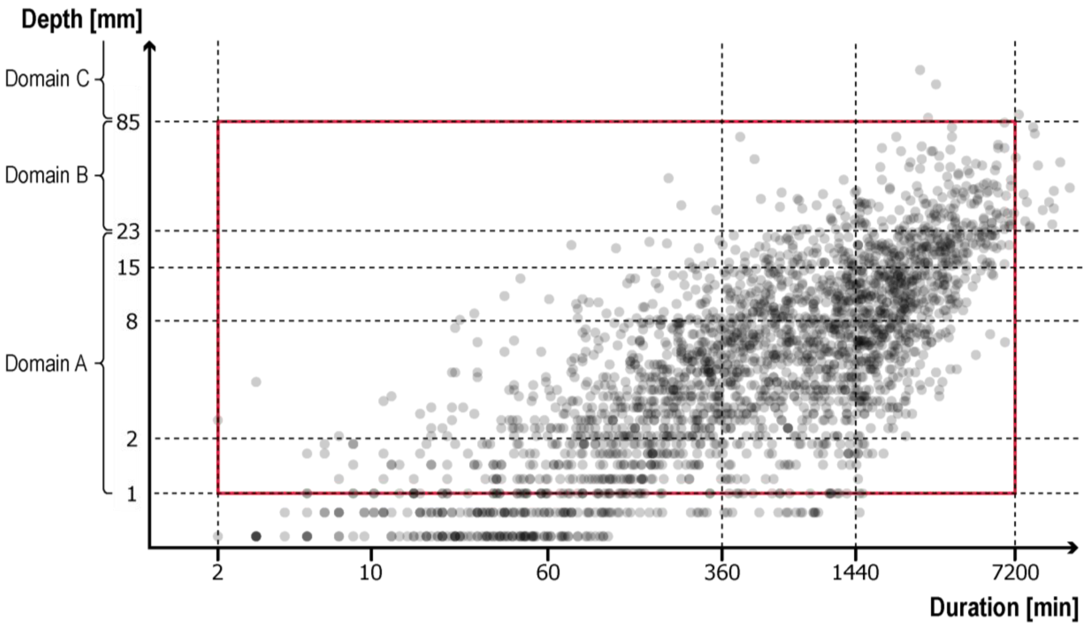
2.1.2. Categorization of Rain Events

First, the return periods of relevance to amenity and utility values were considered. This resulted in the following categories, where the first three are assumed relevant to amenity values and the last two to utility values:

(1).

From 1 mm to once per week;

(2).

From once per week to twice per month;

(3).

From twice per month to once per month;

(4).

From once per month to once every two months; and

(5).

From once every two months to once every 10 years.

The lower boundary for individual events considered was set at 1 mm since this typically reflect the initial loss of the system.

Then, to identify the relevant rain depths and rain duration, we first used the median plotting position [39] to determine which category of return period the individual rain events of the 36-year rain record belonged to, based on their ranking:

$$T_{median}=\frac{T+0.4}{rank-0.3}$$

(1)

where T_Median is the return period, T is the length of the time series, and rank is the rank number of the given event based on magnitude.

Based on this, the return periods were converted into depth intervals, by calculating the minimum and maximum rain depths observed within each category.

To finally create categories of event durations the following three intervals were considered:

(1).

Under 6 h;

(2).

Between 6 and 24 h; and

(3).

Above 24 h.

In practice, the first category was also bound by a minimum duration of 2 min and the last category by a maximum duration of five days.

2.1.3. Selection of Characteristic Rain Events (CREs)

For each of the 15 categories of rain events (five depth intervals times three duration intervals), we selected a statistically representative CRE based on the distribution of rainfall intensities. Firstly, we produced a distribution of rainfall intensities for each rain event by ranking all the recorded one-minute intensities in descending order. Secondly, we calculated the mean of the intensities for each rank to produce a mean distribution of intensities, creating a fictive mean rain event. Finally, we found the CRE among the actual rain events by least square optimization against the fictive mean rain event, also weighing in the length of the event as:

$$\min \left(SSQ\right)=\min \left({{\displaystyle \sum }}_{i=1}^N\frac{{\left(y_i-\widehat{y_i}\right)}^2}{N}\right)$$

(2)

where y_i is the event rainfall intensity at rank step i of the ranked event, ŷ_i is the mean rainfall intensity at rank step i of the ranked events, and N is the number of time steps in the event.

The observed rain event that comes closest to the fictive mean, i.e., has the “most average” distribution of intensities, was identified as the CRE for its category.

2.2. Case Study

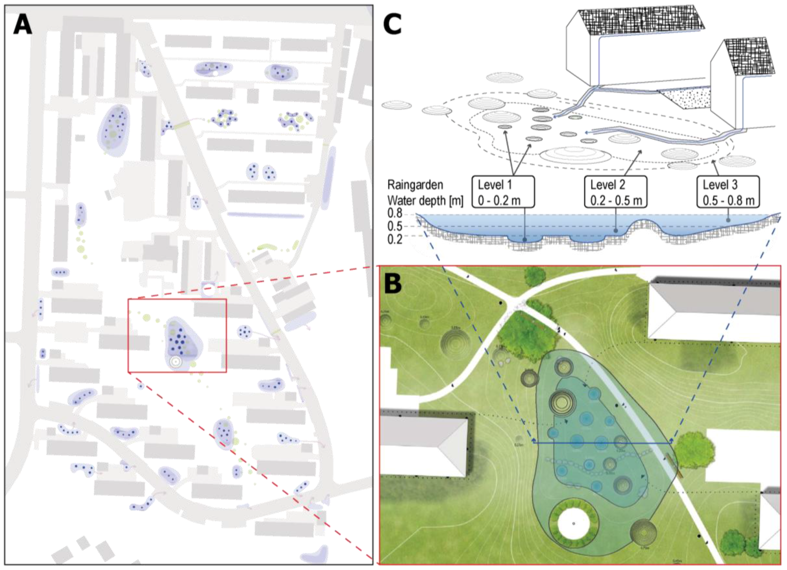
2.2.1. Context of Case Study and Design Suggested

The case used to demonstrate the application of CREs is a stormwater management project of 10 ha in the city of Ballerup in Greater Copenhagen, Denmark (Figure 1), aiming to alleviate problems with frequent flooding. The project was conducted by the German architectural office Gruppe F. The suggested solution includes retention and infiltration of stormwater runoff in green areas between houses, with no discharge from the area. Water droplets on a smooth surface inspired the design, which consists of a simple grass landscape with small circular pools and hills that change their appearance depending on water levels. It was the designers’ intention to not only secure the area from flooding, i.e., meet the utility performance goal, but at the same time “stage” the rainwater on the big lawns of the area and create a design that changes its appearance with the size of the rains, i.e., harvest amenity values too. The necessary retention volume was calculated using a simple spreadsheet for SCMs provided by the Water Pollution Committee of the Society of Danish Engineers [40].

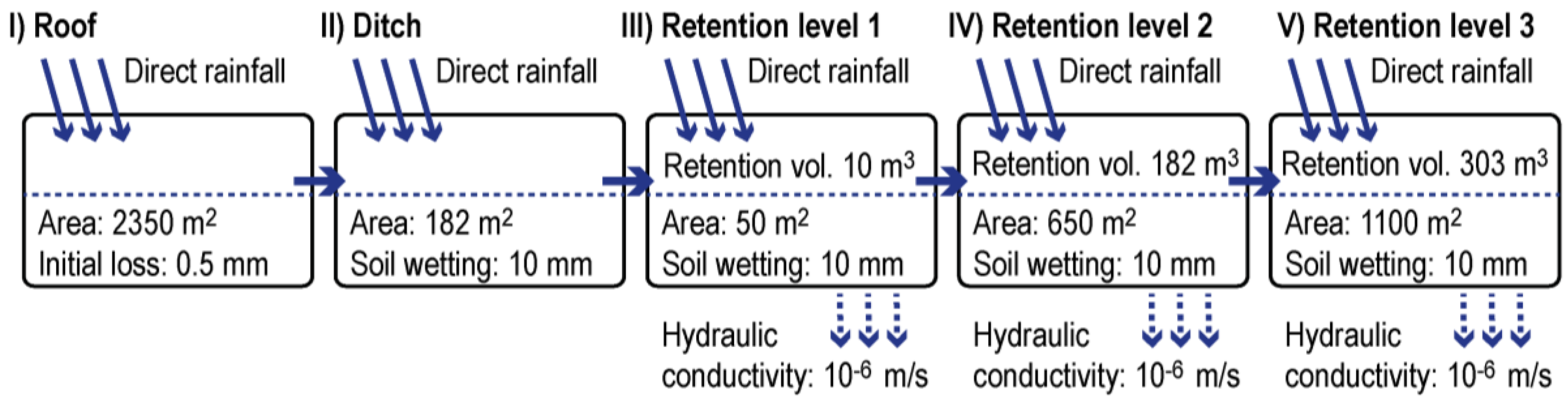
2.2.2. Hydrological Model of Rainwater Flow through Retention Units

A simple mathematical model was developed to describe the flow of stormwater runoff through the retention system described above to provide a dynamic picture of how much water will be visible in the system over the course of a CRE. As illustrated in Figure 2, the model is based on the following sequence of processes explained using the case area: mathematical models of retention units are included in most of the major software packages for simulating drainage systems (e.g., [41,42,43]), and more detailed stand-alone models have also been developed (e.g., [44,45]). However, for our purpose, the complexity of these models was unnecessary and unwanted. Rather, a simplified process expression was developed in order to achieve a fast and robust model focused on producing a chronology of visible water level during single rain events. The processes included in our retention model are illustrated in Figure 2. The sequence of processes is as follows:

(1).

Rain falls on a roof surface, where it is first “lost” to initial wetting of the surface; excess water is conveyed to the ditch.

(2).

In the ditch, runoff from the roof is added to rainwater falling directly in the ditch; again, water is first “lost” to wetting of the surface and the uppermost layer of the soil due to infiltration. Excess water is conveyed to the lowest, level 1 of the retention area.

(3).

In level 1 of the retention area, water from the ditch is added to rainwater falling directly in the retention area. Again, an initial “loss” to wetting of the surface and the uppermost soil layer is removed first. Excess water is infiltrated into the deeper soil, at a rate that is not allowed to exceed the hydraulic conductivity of the native soil multiplied with the bottom area of the level. Excess water is accumulated in the level.

(4).

If the accumulated rainwater in the retention level 1 exceeds the maximum depth of the level, it spills over to the larger level 2, where the same (area-adjusted) processes of wetting and infiltration take place.

(5).

Similarly, if the accumulated water in retention level 2 exceeds the maximum depth of the level, it spills over to level 3, where the same processes of wetting and infiltration take place.

3. Results

3.1. Categorization of Rainfall Depths

The categories of rainfall depths as derived from boundaries defined by return periods (representative for Greater Copenhagen) are presented in

Table 1. Categories of rainfall depths resulting from analysis of the Danish rainfall record with category boundaries as shown. T_max stands for return period representing the upper boundary of each category.

Category Description	Tmax (Year)	Depth Interval (mm)
A rain event that occurs between once every two months and once every 10 years (upper limit of domain B)	10	23–85 mm
A rain event that occurs between once per month and once every two months (lower limit of Domain B and upper limit of domain A)	0.2	15–23 mm
A rain event that occurs between twice per month and once per month	0.1	8–15 mm
A rain event that occurs between once per week and twice per month	0.05	2–8 mm
A rain event that occurs once per week or more often	0.02	1–2 mm

and related to the domains shown in Figure 3.

Intersecting rainfall depth intervals with rain event duration intervals yielded the categories that are illustrated with straight dotted lines in Figure 3. Each dot in the figure represents one rain event, plotted as depth versus duration. The figure shows that depth and duration are correlated. The figure also reveals that some categories are more populous than others for each depth interval. Note that four rain events in the time series fall beyond the chosen intervals of depth (they belong to domain C of the 3PA), and 17 events fall beyond the chosen intervals of event duration (they are longer than five days, 7200 min); these events are excluded from the subsequent analyses.

3.2. The Influence of Aggregation Threshold

Figure 4 shows the distribution of rain events among the five categories of rainfall depth when using three different dry weather durations as threshold values for the event aggregation (12, 24 and 48 h). The individual events (grey lines) are plotted by ranking the rainfall intensities for each minute of the events in descending order (as explained in the introduction); the black lines represent the mean intensity event and the red lines represent the most characteristic event (as determined by Equation (2)). The figure shows that the number of events (NoE) decreases with increasing dry weather threshold length. However, the mean aggregated event duration (μ) and the corresponding standard deviation of this (σ) do not change as noticeably between the different dry weather threshold values. Hence, it was concluded that the choice of CREs is relatively insensitive to choice of dry weather threshold length, and for the rest of the study only rain events resulting from using the threshold value of 24 h of no rain between events are considered.

3.3. Selection of CREs

Figure 5 shows all rain events categorized according to both rainfall depth and event duration plotted in the same way as Figure 4. As in Figure 3, this reveals a general trend of depth and duration to be correlated such that deeper events are also longer events. We chose the five final CREs as the CRE of the most populous duration interval within each depth interval, as indicated by the highlighted boxes in the figure, with one exception: for the second depth interval (2–8 mm), the first duration interval is slightly more populous than the second, however all three intervals contains numerous events, and therefore we found that the middle interval is most representative for all three intervals.

The main properties of the final five CREs are summed up in

Table 2. Main properties of the final five CREs for Greater Copenhagen. T_max stands for return period of the upper boundary of the category that the CRE represents. Share of events reflects the relative number of events that fall within the category that the CRE was selected from, compared to the total number of events included in the analysis.

CRE	Tmax (Year)	Share of Events (%)	Depth (mm)	Duration (min)	Duration (day:h:min)
5	10	8	42.4	2642	1:20:02
4	0.2	11	21.4	4396	3:01:16
3	0.1	21	13.4	2144	1:11:44
2	0.05	49	6.0	937	0:15:37
1	0.02	11	1.8	74	0:01:14

. For example, CRE 1, the rain event that can be said to represent a typical weekly recurring rain in Greater Copenhagen, is a very mild rain with only 1.8 mm of rainwater falling in just over an hour. CRE 2 can be said to be the most representative of all the CREs as it represents the largest share of all events. To understand the rainfall dynamics of the CREs, practitioners should observe the chronology of the events (as done in Figure 7).

3.4. Check for Seasonal Distribution

The seasonal distribution of events within each category was investigated to assess if there is any apparent seasonality in the selected CREs. Figure 6 plots the percent of events in each category that falls within each season. The figure shows that, in the categories from which the final CREs were chosen, which include a large number of events, the events seem to be distributed relatively evenly across seasons. Uneven distribution of events is mainly found where there are few events and for the most infrequent events. As such, the CREs represent events that can happen all year round in Greater Copenhagen.

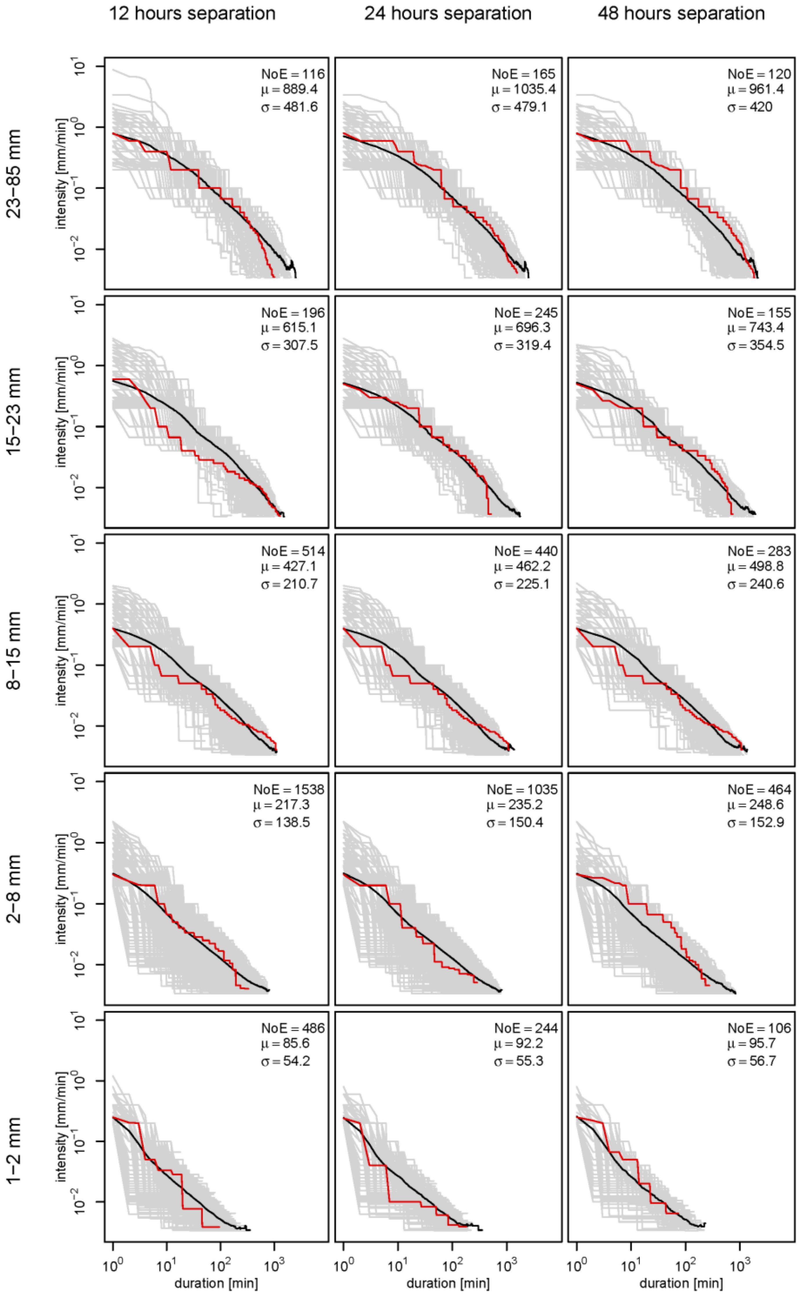
3.5. Flow of CREs through a Retention Unit

Results of running the five CREs through the simple hydrological model are shown in Figure 7. For each of the five CREs, the figure includes from left to right: (1) a chart displaying the partition of rainwater into a part that for some time is visible in the retention area (Figure 1) and a part that immediately “disappears” due to wetting and infiltration; (2) a chronology of rainfall intensity and depth of visible water in the retention area; and (3) a map of the extent of visible water at the peak of the water level.

Figure 7 shows that, for CRE 1, the rain falls in a continuous manner for about one hour, and results in a maximum of about 5 cm of visible water in the smallest ponds of the retention area (level 1), with visible water lasting about 10 h in total. The amount of water that at any time during the event becomes visible corresponds to about 40% of the total rainfall volume, with 60% of the water “disappearing” immediately due to wetting and infiltration.

CRE 2 is composed of three peaks with a few hours between, of which the first peak “disappears” completely, i.e., the entire volume is lost to wetting and infiltration without any visible accumulation of water. The wetting effect is however conserved, so the second peak of the event immediately results in visible water accumulating in level 1 and rather quickly filling it up and spilling over into level 2. Because of the large area in level 2 and thus associated large losses, it requires large volumes of rain to achieve any visible water at this level, which this event does not deliver. As soon as the rain stops, the water level starts dropping steadily, with the exception of a little rise following the third peak of the aggregated rain. Compared to CRE 1, a larger part (50%) of the total rainfall volume becomes visible during the event.

CRE 3 can also be roughly divided into three parts, with the first part delivering a volume large enough to almost fill level 1 of the retention area, and the second part spilling into level 2 and “disappearing” there completely, like in CRE 2. Again, this is followed by a pause where the water level drops well below level 2 followed by a little re-rise caused by the last part of the rain event. Even though more water spills from level 1 to level 2 compared to CRE 2, it is distributed over a longer duration resulting in larger losses due to infiltration, preventing visible water in level 2 and a smaller share (35%) of this CRE being visible.

CRE 4 is a much longer event than CRE 3, including a long period of steady rain, halfway into which the accumulated volume saturates the losses in level 2 and a little water becomes visible across this larger area. However, the effective infiltration in the large area of unit 2 is significantly larger than in the smaller area of unit 1, and the intensity of CRE 4 is not enough to deliver significantly more rain than what is continuously lost to infiltration. Therefore, the water level in unit 2 does not increase substantially above the surface at any point during the event. The percent of visible water increases slightly (38%) compared with CRE 3.

CRE 5 represents a significantly less frequent rain event than CREs 1–4 (belonging to domain B of the 3PA). It includes periods of significantly more intensive rainfall. Consequently, CRE 5 rather quickly fills up level 1 and at the second large peak of the event also quickly matches the losses of level 2 resulting in a significant depth of visible water across the large area of this level. This also entails that this CRE has the largest share of water that turns visible (56%).

4. Discussion

4.1. Selection of CREs

The methodology of selecting CREs places weight on the following characteristics of rain events: their return period (frequency), their duration (aggregated), their total volume (directly linked to the return period and duration) and their intensities. All of these characteristics can be assessed mathematically from standard high-resolution rain gauge data, and it is therefore feasible to select historical events based on these characteristics. However, rain events can be characterized in additional ways, for example with regards to the weather pattern that produced them (which would influence the subjective perception of the event) or the antecedent moisture level in the soil (which would influence how fast the rainwater infiltrates into the soil and how much rainwater becomes visible). Such characteristics cannot be extracted from the rain gauge data alone; assessing them would require additional data sources and/or simulation models. Hence, when we label the selected rain events as “characteristic”, we are limited to the characteristics that can be calculated from the rain data alone, and cannot claim that they are “characteristic” in all possible aspects.

Regarding the selection of return periods, the choice was subjective and can be debated, but this choice can also easily be changed to suit other preferences and objectives. One advantage of the present choice is its anchor in a previous definition of the domains of the 3PA for Denmark, thus setting it within a framework that has a proven ability to bridge between different professions working with managing rainwater in cities.

Regarding the selection of event durations, the choice was influenced by the length of the events that resulted from the aggregation method. The raw data could have been used (with an aggregation threshold of one hour), which would have resulted in shorter events in all categories. With the intended use of the CREs (for staging water in SCMs), this would have been less appropriate, since a single (non-aggregated) CRE would often not result in a distinct response in the SCM. Instead, the response would to a much higher degree depend on the previous rain events, thus weakening the power of interpretation that can be assigned to each CRE.

Regarding the intensities’ characteristic, the choice was based on the ranked rainfall intensities within the (aggregated) events, disregarding any dry periods. With this simplification, the full variability in the dynamics within the different events cannot be addressed. However, it is considered a reasonable choice, since any dry period within the event will necessarily be smaller than the separation threshold (of 24 h) and hence not be of great influence on the response of the SCM.

The Danish rainfall pattern is unique in its relatively even distribution all year round (mean rainfall depth in the driest month is approximately 40 mm, compared to approximately 80 mm in the wettest month). Seasonal variation manifests itself in the less frequent events, with spring and summer thunderstorms being responsible for intensive cloudbursts that challenge urban drainage systems. With the focus on the more frequent “daily” rain events in this study, this phenomenon has little impact, as is demonstrated in the check for seasonal distribution (Figure 6). In other climates where seasons play a larger role than in Denmark (e.g., those with a distinct dry season), the selection methodology would have to be adapted to reflect this (e.g., by defining a return period of a CRE as “once per week within the wet season”) to ensure realistic communication regarding when to expect visible water in the SCM.

4.2. Simulating Flow of a CRE in an SCM

The presented model of flow through a retention area was intended to provide an example of how the dynamics of CREs will result in different levels of visible water over time in an SCM. One of the important simplifying choices made in the model is the use of hard coded values for so-called “initial losses” (including wetting of the roof surface, the grassed surfaces and the uppermost soil layers). This means that every event simulation starts with the same conditions, which were assessed to represent average year-round moisture conditions in Denmark. However, in reality, there will be significant differences in antecedent moisture conditions between, e.g., summer and winter (with low temperatures and high humidity in winter entailing that there are much smaller initial losses and hence more visible water can be expected). Overcoming this barrier would require a model that includes evapotranspiration, run in continuous mode for several years, and then analyzing the response events rather than the rain events. This is considerably more resource demanding than the modeling approach undertaken here, and it is believed that the added value does not outweigh the extra effort. A compromise could be to run simulations with varying values of initial losses to reflect different conditions, e.g., seasons, which might be a reasonable additional step in more ambitious projects.

The model is tailored to the case study, and applying it to a different SCM design would require some adaptation. In other words, the model, unlike the CREs, is not an “off the shelf” tool that a designer can use immediately. However, the principles behind it are, as mentioned before, rather simple, and the method could potentially be included as an add-on in design tools used by landscape architects.

4.3. Usefulness of CREs

CREs have been tested on a real-life case study but not in direct collaboration with the designers; therefore, it is not possible to conclude on the usefulness to designers of CREs in the design phase. Possible advantages may include:

(1).

A simple table such as Table 1 will provide useful key figures that can aid the designer in proportioning different sub-volumes within an SCM that can stage frequent rain events.

(2).

Taking a step further from summary properties of CREs to inspection of a graphical chronology of the different CREs, as included in Figure 7, may add further benefits. For example, it promotes an understanding of rain events in the context of SCMs as being aggregated over longer periods of alternating rain/no rain rather than being single “showers”. Furthermore, such a chronology gives an idea about the varying rainfall intensities during frequent rain events, which are generally much lower than those used to set the overall dimensions of the transport elements of the SCM. This knowledge can be used to design transport elements that stage also frequent flows.

(3).

Taking the last step from inspection of the chronology of the CREs to simulating the resulting chronology of visible water in an SCM design gives the designer a powerful interactive tool to optimize the design. Small changes in the shape of an SCM can lead to large improvements in how often water is visible. The case study was already designed with the goal of staging frequent rains, by making “depressions within depressions”, i.e., sub-volumes, and the simulation shows that this was successfully achieved.

Simulating the hydrological fate of the different CREs confirms the importance of initial losses. A general lesson that can be learned from this is that in order to stage water during frequent rain events, runoff needs to be concentrated in rather small areas, or sub-volumes (and not spread out evenly over large areas). However, this strategy may entail other challenges: as can be seen from the chronology, the small units empty slowly (much slower than the recommended 24 h), calling for vegetation with a huge amplitude in soil humidity tolerance. It would be necessary to strike a balance between concentrating the water in small enough depressions to make it visible, while also making sure that this does not result in unattractive mud holes.

5. Conclusions

In this study, a recognized need for a simple design tool that can help landscape architects in staging water in SCMs is addressed, by suggesting the use of a collection of historical rain events that can be said to be characteristic of the location in question and of the frequency at which designers expect rainwater to be visible in the SCM. A methodology is developed for choosing such events from a rain gauge data series, and it is applied to a series from Greater Copenhagen, Denmark, presenting five final Characteristic Rain Events (CREs) for this climate. A simple model to describe water flow through an SCM based on a retention area in a specific case study was also developed; it was used to investigate how much visible water was induced by each of the five CREs. It is concluded that: (1) it is possible to identify characteristic rain events in a statistically sound way; (2) basic knowledge about the frequency, duration and depth of such events may significantly increase designers’ awareness towards the types of rainfall relevant to target when designing for water visibility; and (3) a simple hydrological model of flow through an SCM may additionally enhance the usefulness of the CREs by illustrating how well a specific design is able to stage rainwater.

References

1. Fletcher, T.D.; Shuster, W.; Hunt, W.F.; Ashley, R.; Butler, D.; Arthur, S.; Trowsdale, S.; Barraud, S.; Semadeni-Davies, A.; Bertrand-Krajewski, J.-L.; et al. SUDS, LID, BMPs, WSUD and more—The evolution and application of terminology surrounding urban drainage. Urban Water J. 2015, 12, 525–542. [Google Scholar] [CrossRef]
2. De Sousa, M.R.C.; Montalto, F.; Spatari, S. Using Life Cycle Assessment to Evaluate Green and Grey Combined Sewer Overflow Control Strategies. J. Ind. Ecol. 2012, 16, 901–913. [Google Scholar] [CrossRef]
3. Moore, T.L.; Hunt, W.F. Ecosystem service provision by stormwater wetlands and ponds—A means for evaluation? Water Res. 2012, 46, 6811–6823. [Google Scholar] [CrossRef] [PubMed]
4. Sarkar, C.; Webster, C.; Pryor, M.; Tang, D.; Melbourne, S.; Zhang, X.; Jianzheng, L. Exploring associations between urban green, street design and walking: Results from the Greater London boroughs. Landsc. Urban Plan. 2015, 143, 112–125. [Google Scholar] [CrossRef]
5. Belmeziti, A.; Cherqui, F.; Tourne, A.; Granger, D.; Werey, C.; Le Gauffre, P.; Chocat, B. Transitioning to sustainable urban water management systems: How to define expected service functions? Civ. Eng. Environ. Syst. 2015, 1–19. [Google Scholar] [CrossRef]
6. Zhou, Q. A Review of Sustainable Urban Drainage Systems Considering the Climate Change and Urbanization Impacts. Water 2014, 6, 976–992. [Google Scholar] [CrossRef]
7. Echols, S.; Pennypacker, E. From Stormwater Management to Artful Rainwater Design. Landscape 2008, 27, 268–290. [Google Scholar] [CrossRef]
8. Zhou, Q.; Panduro, T.E.; Thorsen, B.J.; Arnbjerg-Nielsen, K. Adaption to extreme rainfall with open urban drainage system: An integrated hydrological cost-benefit analysis. Environ. Manag. 2013, 51, 586–601. [Google Scholar] [CrossRef] [PubMed] [Green Version]
9. Backhaus, A.; Fryd, O. The aesthetic performance of urban landscape-based stormwater management systems: A review of twenty projects in Northern Europe. J. Landsc. Archit. 2013, 8, 52–63. [Google Scholar] [CrossRef]
10. Backhaus, A.; Dam, T.; Jensen, M.B. Stormwater management challenges as revealed through a design experiment with professional landscape architects. Urban Water J. 2012, 9, 29–43. [Google Scholar] [CrossRef]
11. Bolund, P.; Hunhammar, S. Ecosystem services in urban areas. Ecol. Econ. 1999, 29, 293–301. [Google Scholar] [CrossRef]
12. Fisher, B.; Turner, R.K.; Morling, P. Defining and classifying ecosystem services for decision making. Ecol. Econ. 2009, 68, 643–653. [Google Scholar] [CrossRef]
13. Gómez-Baggethun, E.; Barton, D.N. Classifying and valuing ecosystem services for urban planning. Ecol. Econ. 2013, 86, 235–245. [Google Scholar] [CrossRef]
14. Tzoulas, K.; Korpela, K.; Venn, S.; Yli-Pelkonen, V.; Kamierczak, A.; Niemela, J.; James, P. Promoting ecosystem and human health in urban areas using Green Infrastructure: A literature review. Landsc. Urban Plan. 2007, 81, 167–178. [Google Scholar] [CrossRef]
15. City of Copenhagen. Climate Adaptation & Urban Nature; City of Copenhagen: Copenhagen, Denmark, 2016; p. 152. Available online: http://www.ameko.dk/blog/2016/6/20/copenhagen-think-tank-on-climate-adaption-urban-nature (accessed on 17 August 2017).
16. Echols, S.; Pennypacker, E. Artful Rainwater Design: Creative Ways to Manage Stormwater, 1st ed.; Island Press: Washington, DC, USA, 2015. [Google Scholar]
17. Rittel, H.W.J.; Webber, M.M. Dilemmas in a general theory of planning. Policy Sci. 1973, 4, 155–169. [Google Scholar] [CrossRef]
18. Andersson, S.I. Landscape architecture at the Royal Danish Academy of Fine Arts, Copenhagen, Denmark. Landsc. Urban Plan. 1994, 30, 169–177. [Google Scholar] [CrossRef]
19. Lawson, B. How Designers Think—The Design Process Demystified; Architectural Press: Oxford, UK, 2006. [Google Scholar]
20. Schön, D.A. The Reflective Practitioner—How Professionals Think in Action; Ashgate Publishing Limited: London, UK, 2003. [Google Scholar]
21. Von Seggern, H.; Werner, J.; Grosse-Bächle, L. Creating Knowledge—Innovation Strategies for Designing Urban Landscapes; Jovis Verlag: Berlin, Germany, 2008. [Google Scholar]
22. Gehl, J.; Svarre, B. How to Study Public Life; Island Press: Washington, DC, USA, 2013. [Google Scholar]
23. Lynch, K. The Image of the City; Harvard University Press: Cambridge, MA, USA, 1960. [Google Scholar]
24. Dreiseitl, H.; Grau, D.; Ludwig, K.H.C. Waterscapes—Planning, Building and Designing with Water; Birkhäuser Verlag: Basel, Switzerland, 2001. [Google Scholar]
25. Sieker, H.; Sieker, F.; Kaiser, M. Dezentrale Regenwasserbewirtschaftung im Privaten, Gewerblichen und Kommunalen Bereich-Grundlagen und Ausführungsbeispiele; Fraunhofer IRB Verlag: Stuttgard, Germany, 2006. [Google Scholar]
26. Dubois, C.; Cloutier, G.; Potvin, A.; Adolphe, L.; Joerin, F. Design support tools to sustain climate change adaptation at the local level: A review and reflection on their suitability. Front. Archit. Res. 2015, 4, 1–11. [Google Scholar] [CrossRef]
27. Woods-Ballard, B.; Kellagher, R.; Martin, P.; Jefferies, C.; Bray, R.; Shaffer, P. The SUDS Manual; CIRIA Classic House: London, UK, 2007. [Google Scholar]
28. Elliott, A.; Trowsdale, S. A review of models for low impact urban stormwater drainage. Environ. Model. Softw. 2007, 22, 394–405. [Google Scholar] [CrossRef]
29. Jayasooriya, V.M.; Ng, A.W.M. Tools for Modeling of Stormwater Management and Economics of Green Infrastructure Practices: A Review. Water Air Soil Pollut. 2014, 225, 2055. [Google Scholar] [CrossRef]
30. Lerer, S.M.; Arnbjerg-Nielsen, K.; Mikkelsen, P.S. A Mapping of Tools for Informing Water Sensitive Urban Design Planning Decisions—Questions, Aspects and Context Sensitivity. Water 2015, 7, 993–1012. [Google Scholar] [CrossRef]
31. Sørup, H.J.D.; Georgiadis, S.; Gregersen, I.B.; Arnbjerg-Nielsen, K. Formulating and testing a method for perturbing precipitation time series to reflect anticipated climatic changes. Hydrol. Earth Syst. Sci. 2017, 21, 345–355. [Google Scholar] [CrossRef]
32. Koutsoyiannis, D.; Baloutsos, G. Analysis of a long record of annual maximum rainfall in Athens, Greece, and design rainfall inferences. Nat. Hazards 2000, 22, 29–48. [Google Scholar] [CrossRef]
33. Ahern, J. From fail-safe to safe-to-fail: Sustainability and resilience in the new urban world. Landsc. Urban Plan. 2011, 100, 341–343. [Google Scholar] [CrossRef]
34. Gallo, C.; Moore, A.; Wywrot, J. Comparing the adaptability of infiltration based BMPs to various U.S. regions. Landsc. Urban Plan. 2012, 106, 326–335. [Google Scholar] [CrossRef]
35. Rivard, G. Small Storm Hydrology and BMP Modeling with SWMM5. J. Water Manag. Model. 2010. [Google Scholar] [CrossRef]
36. Fratini, C.F.; Geldof, G.D.; Kluck, J.; Mikkelsen, P.S. Three Points Approach (3PA) for urban flood risk management: A tool to support climate change adaptation through transdisciplinarity and multifunctionality. Urban Water J. 2012, 9, 317–331. [Google Scholar] [CrossRef] [Green Version]
37. Sørup, H.J.D.; Lerer, S.M.; Arnbjerg-Nielsen, K.; Mikkelsen, P.S.; Rygaard, M. Efficiency of stormwater control measures for combined sewer retrofitting under varying rain conditions: Quantifying the Three Points Approach (3PA). Environ. Sci. Policy 2016, 63, 19–26. [Google Scholar] [CrossRef] [Green Version]
38. Beecham, S.; Chowdhury, R. Effects of changing rainfall patterns on WSUD in Australia. Proc. Inst. Civ. Eng. 2012, 165, 285–298. [Google Scholar] [CrossRef]
39. Rosbjerg, D. Defence of the Median Plotting Position, Progress Report—Institute of Hydrodynamics and Hydraulic Engineering; Technical University of Denmark: Lyngby, Denmark, 1988. [Google Scholar]
40. Water Pollution Committee of the Society of Danish Engineers. Sizing of SCMs. Dimensionering af LAR-anlæg. Available online: https://ida.dk/sites/default/files/SVK_LAR-Dimensionering_v1_0.pdf (accessed on 1 September 2017).
41. DHI. Mike Urban Collection System; DHI: Hørsholm, Denmark, 2016. [Google Scholar]
42. eWater. MUSIC Documentation and Help 6.0; eWater: Melbourne, Australia, 2014. [Google Scholar]
43. Rossman, L.A. Modeling Low Impact Development Alternatives with SWMM. J. Water Manag. Model. 2010, 167–182. [Google Scholar] [CrossRef]
44. Brown, R.A.; Skaggs, R.W.; Hunt, W.F. Calibration and validation of DRAINMOD to model bioretention hydrology. J. Hydrol. 2013, 486, 430–442. [Google Scholar] [CrossRef]
45. Roy-Poirier, A.; Filion, Y.; Champagne, P. An event-based hydrologic simulation model for bioretention systems. Water Sci. Technol. 2015, 72, 1524–1533. [Google Scholar] [CrossRef] [PubMed]
Figure 1. (A) Overview map showing the retention areas with small pools designed for 1/2-year rain events (return period 0.5 year), larger pools for the five-year rain event (return period 5 years) and overflow zones for the 100-year rain event (return period 100 years), where excess soil is used to form small hills that protrude from the temporary ponds in wet conditions; (B) map of one retention zone; and (C) cross-section through the area and 3D-concept illustration.
Sustainability 09 01793 g001
Figure 2. Flow process of rainwater from roof runoff through retention units included in model for calculating water dynamics by means of CREs.
Sustainability 09 01793 g002
Figure 3. Individual rain events in the Copenhagen time series (36 years) plotted as a function of duration and depth, with dashed lines indicating the 15 categories of duration and depth intervals.
Sustainability 09 01793 g003
Figure 4. Rain events divided into categories based on rainfall depth (rows) and dry weather aggregation threshold value (columns), plotted as a function of rainfall intensity from most to least intense minute during the event. Grey lines represent the historical events in each category, black lines represent the calculated mean intensity event for each category, and red lines represent the historical event that most resembles the mean event of its category. NoE = Number of events; μ = mean event duration; σ = standard deviation of the event duration.
Sustainability 09 01793 g004
Figure 5. Individual rain events, divided in categories based on rainfall depth (rows) and rain event duration (columns) based on 24 h aggregation threshold, ranked from most to least intense minute. Grey lines represent the historical events in each category, black lines represent the mean intensity event for each category, and red lines represent the historical event that most resembles the mean event of its category. NoE = Number of events; μ = mean event duration; σ = standard deviation of the event duration.
Sustainability 09 01793 g005
Figure 6. Seasonal distribution of the considered rain events split into same depth-duration categories as in Figure 5.
Sustainability 09 01793 g006
Figure 7. Illustration of results from running the five CREs through a simplified hydrological model of the retention area of the case study (Figure 1). Leftmost chart displays the partition of the total event volume between water that immediately disappears due to wetting or infiltration and water that accumulates on the surface and becomes visible. Central chart displays timeline of rainfall intensity during the CRE and resulting depth of visible water in the retention area. Rightmost part shows a map-based illustration of the areal extent of the visible water at the peak of visibility during the event.
Sustainability 09 01793 g007